Liquid stability in a model for ortho-terphenyl

Abstract

We report an extensive study of the phase diagram of a simple model for ortho-terphenyl, focusing on the limits of stability of the liquid state. Reported data extend previous studies of the same model to both lower and higher densities and to higher temperatures. We estimate the location of the homogeneous liquid-gas nucleation line and of the spinodal locus. Within the potential energy landscape formalism, we calculate the distributions of depth, number, and shape of the potential energy minima and show that the statistical properties of the landscape are consistent with a Gaussian distribution of minima over a wide range of volumes. We report the volume dependence of the parameters entering in the Gaussian distribution (amplitude, average energy, variance). We finally evaluate the locus where the configurational entropy vanishes, the so-called Kauzmann line, and discuss the relative location of the spinodal and Kauzmann loci.

I Introduction

Recent years have seen a strong development of numerical and theoretical studies of simple liquid models, attempting to develop a thermodynamic description based on formalisms which could be extended to deal also with out-of-equilibrium (glassy) states speedy ; kurchan ; mezpar ; angmk ; teo ; franz ; leuzzi ; mossa ; soft . Hard spheres, soft spheres, Lennard Jones mixtures and simple molecular liquids speedybook ; speedymolphys ; voivod01 ; scott ; starr01 ; sastry01 ; roberts ; otplungo have been extensively studied. Within the potential energy landscape (PEL) stillingerpes thermodynamic approach, detailed comparisons between numerical data and theoretical predictions have been performed. Estimates of the number $\Omega$ of local minima –basins– as a function of the basin depth and of their shape have been recently evaluated for a few models speedymolphys ; skt99 ; scala00 ; starr01 ; sastry01 ; heuer00 ; voivod01 ; speedyjpc ; otplungo and from the analysis of experimental data stillinger98 ; richert98 ; speedyjpc2 . The PEL approach, which is particularly well suited for describing supercooled liquids, provides a controlled way to extrapolate the thermodynamic properties of the liquid state below the lowest temperature at which equilibrated data can be collected. For example, estimates of the locus where the configurational entropy vanishes, the so-called Kauzmann locus, can be given notakauz ; the Kauzmann locus provides a theoretical limit to the metastable liquid state at low temperatures. Another limit to the liquid state is met on superheating and stretching the liquid, when the nucleation of the gas phase takes place. In this case a convenient way to define the limit of stability of the liquid state against gas nucleation is provided by the spinodal line, i.e., the locus of point where the compressibility diverges pablobook . The Kauzmann line and the spinodal line define the region of phase space where the liquid can exist in stable or metastable thermodynamic equilibrium.

Recent theoretical and numerical work has focused on the thermodynamic relation between these two curves kauzsdt ; sriprl ; soft ; speedypisa ; speedypreprint . A recent thermodynamic analysis speedypisa ; speedypreprint suggests that the spinodal and the Kauzmann loci meet –in the $(P,T)$ plane– with the same slope at a point corresponding to the maximum tension that the supercooled liquid can sustain. Simple models which can be solved analytically, as hard speedybook or soft speedypisa ; scott spheres complemented by a mean field attractive potential, support such prediction. A numerical study of a Lennard Jones mixture is also consistent sriprl .

In this paper we consider the Lewis and Wahnström rigid model for the fragile glass former ortho-terphenyl (OTP) lewis , whose dynamic lewis ; rinaldi ; chong and thermodynamic features otplungo ; lanave have been studied in detail. Our aim is to calculate the spinodal and the Kauzmann lines to estimate the region of stability of the liquid, and study the relation between these two loci.

We improve the data base of phase state points of previous studies otplungo , extending to both lower and higher densities and to higher temperatures. Performing analysis of the pressure-volume relation along several isotherms, we estimate the homogeneous nucleation line and the spinodal curve; we also report upgraded estimates of the statistical properties of the landscape sampled by the liquid. We confirm that at all densities a Gaussian landscape properly models the thermodynamics of the system in the supercooled state. Such agreement gives us confidence in the evaluation of the locus along which the configurational entropy vanishes. We finally discuss the limits and possibilities of an analysis based on the inherent structures thermodynamic formalism. The description of our results is preceded by a short review of the potential energy landscape approach to the thermodynamics of supercooled liquids.

II Background: the free energy in the inherent structures thermodynamic formalism

An expression for the liquid free energy in the range of temperatures where the liquid is supercooled can be given within the PEL formalism. In supercooled states, i.e., when the correlation functions show the two steps behavior typical of the cage effect kob-review ; mct1 , the system’s properties are controlled by the statistical properties of the PEL sds . In the PEL formalism, the potential energy hyper-surface –fixed at constant volume– is partitioned into basins; each basin is defined as the set of points such that a steepest descent path originating from them ends in the same local minimum. The configuration corresponding to the minimum is called inherent structure (IS), of energy $e_{IS}$ and pressure $P_{IS}$. The partition function can be expressed as the sum over all the basins, weighted by the appropriate Boltzmann factor, i.e., as a sum over the single basin’s partition functions. As a result, the Helmholtz liquid free energy $F(T,V)$, at temperature $T$ and volume $V$, can be written as stillingerpes :

$$F(T,V)=E_{IS}(T,V)-TS_{conf}(T,V)+f_{vib}(T,V).$$ (1)

Here, $E_{IS}$ is the average energy of the IS explored at the given $(T,V)$, $f_{vib}$ is the vibrational free energy, i.e., the average free energy of the system when constrained in a basin of depth $e_{IS}$, and $S_{conf}(T,V)$ is the configurational entropy, that counts the number of explored basins. $S_{conf}(T,V)$ is a quantity of crucial interest, both for comparing numerical results with the recent theoretical calculations mezpar ; coluzzi , and to examine some of the proposed relations between dynamics and thermodynamics adam65 ; schultz ; wolynes . Therefore, in order to evaluate the free energy one needs to estimate the three terms of Eq. (1). $E_{IS}(T,V)$ is calculated by means of a steepest descent potential energy local minimization of equilibrium configurations (see Ref. otppisa for details). In fragile liquids the $T$ dependence of $E_{IS}(T,V)$ follows a $1/T$ law heuer ; sastry01 ; starr01 ; otplungo .

The basin free energy $f_{vib}(T,V)$ takes into account both the basin’s shape –curvature– and the system kinetic energy. From the formal point of view, this term is the integral of the Boltzmann factor constrained in a basin, averaged over all the basins with same depth $e_{IS}(T,V)$. Numerically, $f_{vib}$ is evaluated as sum of two contributions: i) a harmonic contribution, which depends on the curvature of the accessed basins corresponding to the minimum at the given $e_{IS}$; ii) an anharmonic contribution, usually approximated as a function of $T$ only. In the case of a rigid molecule model, the harmonic contribution is the free energy associated with a system of $(6N-3)$ independent oscillators of frequency $\omega_{k}$, where the $\omega_{k}$ are the square root of the eigenvalues of the system Hessian matrix –the matrix of the second derivatives of the potential energy– evaluated at the basin minimum (see Ref. otppisa for details). This contribution can be written as notaerrore :

$$f_{harm}(E_{IS},T,V)=\ln\langle\exp\left\{\sum_{i=1}^{6N-3}\ln(\beta\hbar\omega_{i}(e_{IS}))\right\}\rangle^{\prime},$$ (2)

where the symbol $\langle\rangle^{\prime}$ denotes the average over all the basins with the same energy $e_{IS}$. The $E_{IS}$ dependence of $f_{vib}$, in the harmonic approximation, can be parameterized using the expression:

$$\ln\langle\exp\left\{\sum_{i=1}^{6N-3}\ln(\beta\hbar\omega_{i}(E_{IS}))\right\}\rangle^{\prime}=a(V)+b(V)E_{IS}+c(V)E_{IS}^{2}.$$ (3)

The evaluation of $f_{anh}(T,V)$ is described in Ref. otppisa .

Finally, $S_{conf}$ can be calculated as the difference of the (total) entropic part of Eq. (1) and the vibrational contribution to the entropy:

$$S_{conf}(T,V)=S(T,V)-S_{\rm harm}(T,V)-S_{\rm anh}(T,V).$$ (4)

III Background: the Gaussian landscape

In order to evaluate analitically the free energy in the PEL formalism, it is necessary to provide a model for the probability distribution of $e_{IS}$ , i.e., the number $\Omega(e_{IS})de_{IS}$ of basins whose depth lies between $e_{IS}$ and $e_{IS}+de_{IS}$. Among several possibilities, the Gaussian distribution rem ; heuer00 ; sastrynature seems to provide a satisfactory description of the numerical simulations of Refs. sastrynature ; otplungo ; starr01 . The “Gaussian landscape” is defined by:

$$\Omega(e_{IS})de_{IS}=e^{\alpha N}\frac{e^{-(e_{IS}-E_{o})^{2}/2\sigma^{2}}}{(2\sigma^{2})^{1/2}}de_{IS}.$$ (5)

Here, the amplitude $e^{\alpha N}$ accounts for the total number of basins, $E_{o}$ plays the role of energy scale and $\sigma^{2}$, measures the width of the distribution. One can grasp the origin of such distribution invoking the central limit theorem. Indeed, in the absence of a diverging correlation length, in the thermodynamic limit, each IS can be decomposed in a sum of independent subsystems notadistribuzione , each of them characterized by its own value of $e_{IS}$. The IS energy of the entire system, in this case, will be distributed according to Eq. (5).

The assumptions of a Gaussian Landscape (Eq. (5)) and of a quadratic dependence of the basin free energy on $E_{IS}$ (Eq. (3)) fully specify the statistical properties of the model. Thus, it is possible to evaluate the $T$ dependence of $E_{IS}$ and $S_{conf}$. The corresponding expressions are otppisa :

$$E_{IS}(T,V)=\frac{(E_{o}(V)-(b(V)+\beta)\sigma^{2}(V))}{1+2c(V)\sigma^{2}(V)}=A+\frac{B}{T},$$ (6)

where, for convenience, we have defined $A=\frac{E_{o}-b\sigma^{2}}{1+2c\sigma^{2}}$ and $B=\frac{-\sigma^{2}}{k_{B}(1+2c\sigma^{2})}$; and

$$S_{conf}(T,V)/k_{B}=\alpha(V)N-\frac{(E_{IS}(T,V)-E_{o}(V))^{2}}{2\sigma^{2}(V)}.$$ (7)

Note that $E_{IS}$ is linear in $1/T$. The predicted $1/T$ dependence of $E_{IS}$ and the parabolic dependence of $S_{conf}$ has been confirmed in several models for fragile liquids sastrynature ; otplungo ; starr01 .

From the relations above and fits of the numerical data, one obtains: i) the vibrational coefficients $a$, $b$ and $c$ from Eq. (3); ii) the distribution parameters, $E_{o}$ and $\sigma^{2}(V)$ from Eq. (6); iii) the amplitude $e^{\alpha N}$ from Eq. (7). A study of the volume dependence of the parameters $\alpha(V)$, $E_{o}(V)$, and $\sigma^{2}(V)$ , associated with the $V$-dependence of the shape indicators (Eq. (3)), provides a full characterization of the volume dependence of the landscape properties of a model, and offers the possibility of developing an equation of state based on the volume dependence of the statistical properties of the landscape lanave .

Finally, within the Gaussian landscape model, it is possible to exactly evaluate the Kauzmann curve $T_{K}(T,V)$ , the limit for the existence of the liquid. This curve is the locus of points where $S_{conf}$ vanishes, i.e., from Eq. (7),

$$\alpha(V)N-\frac{(E_{IS}(T,V)-E_{o}(V))^{2}}{2\sigma^{2}(V)}=0.$$ (8)

The following expression for $T_{K}(T,V)$ results:

$$T_{K}(T,V)=\frac{B}{(E_{o}-A)\pm\sqrt{2\sigma^{2}\alpha N}},$$ (9)

where the sign to be chosen is the one corresponding to the largest value solution of the equation.

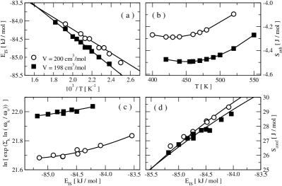
Figure 1: Results of the landscape analysis for the densities $198$ and $200$ cm³/mol (squares and circles symbols respectively): a) average inherent structure energy (symbols) together with the $1/T$ dependence of Eq. (6) (solid line), b) anharmonic contribution to the entropy, c) harmonic free energy $\ln\langle\exp\left\{\sum_{i=1}^{6N-3}\ln(\beta\hbar\omega_{i}(E_{IS}))\right\}\rangle$, d) configurational entropy $S_{conf}$ together with the fits according to Eq. (7).

IV Model and simulations

We studied a system of $343$ Lewis and Wahnström (LW) lewis ortho-terphenyl model molecules, by means of molecular dynamics simulations in the $(N,V,T)$ ensemble. The LW model is a rigid, three-site model with intermolecular site-site interactions described by Lennard Jones potential. The potential parameters are chosen to reproduce OTP properties such as its structure and diffusion coefficient lewis . The integration time step for the simulation was $0.01$ ps. With this model it is possible to reach very long simulation times; such long molecular dynamics trajectories allow us to equilibrate the system at temperatures below the temperature where the diffusion constant reaches values of order $10^{-10}$ cm²/s. We simulated $23$ different densities for several temperatures, for an overall simulation time of order $10$ $\mu$s.

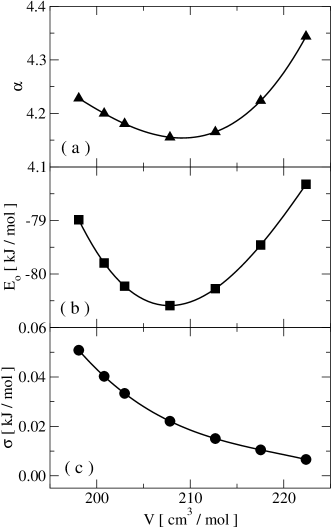
Figure 2: Volume dependence of the Gaussian landscape parameters: a) $\alpha(V)$, b) $E_{o}(V)$, and c) $\sigma^{2}(V)$.

To calculate the inherent structures sampled by the system in equilibrium we perform conjugate gradient energy minimizations to locate the closest local minima on the PEL, with a tolerance of $10^{-15}$ kJ/mol. For each thermodynamical point we minimize at least $100$ configurations, and we diagonalize the Hessian matrix of at least $50$ configurations to determine the density of states. The Hessian is calculated choosing for each molecule the center of mass and the angles associated with rotations around the three principal inertia axis as coordinates.

Further details on the numerical techniques used can be found in Ref. otplungo .

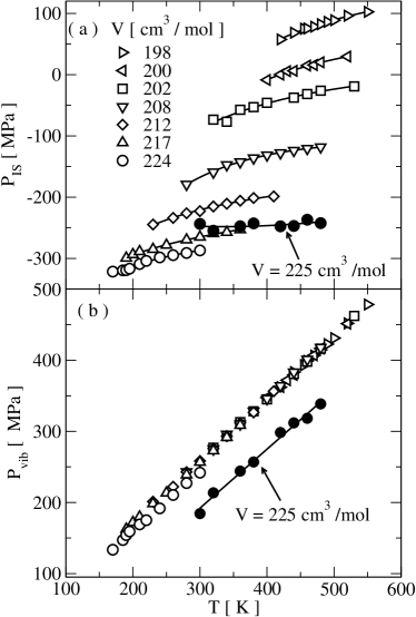
Figure 3: a) Inherent structure pressure, $P_{IS}$. The IS pressure gets more negative on decreasing density, until a sudden jump upward takes place at around $225$ cm³/mol. The jump signals that, during the minimization procedure (at constant volume), the maximum tensile strength has been overcome and a cavitation phenomenon has taken place. b) vibrational pressure, $P_{vib}$. $P_{vib}$ is almost density independent. Only at densities close to the Sastry density, a $V$ dependence is observed.

V Potential energy landscape properties

An analysis of the statistical properties of the landscape for the LW ortho-terphenyl model has been recently performed in Ref. otplungo . Here we expand such analysis to lower and higher densities, with the aim of exploring the region of phase diagram where the steep repulsive part of the potential is more relevant, and study the location of the liquid spinodal line and of the Sastry density sripre ; sriprl . The larger density range considered allows us to estimate the volume dependence of the landscape parameters with great precision.

Figure 4: Volume dependence of the total pressure $P$, inherent structures pressure $P_{IS}$, and vibrational pressure $P_{vib}$ for the isotherm $T=320$ K. The total pressure $P$ is monotonically decreasing, as expected for a system in equilibrium in the stable liquid phase. The IS pressure shows instead a minimum around $V=222$ cm³/mol, suggesting that, during the minimization process, a cavitation process has taken place in the $V=225$ cm³/mol sample. As a result, the significant drop observed in $P_{vib}$ is an artifact induced by cavitation.

The four panels of Fig. 1 show the results of the landscape analysis for two of the additional densities ($198$ and $200$ cm³/mol), with the aim of confirming the possibility of describing the numerical data with the Gaussian landscape model discussed above. Similar data for other five densities can be found in Ref. otplungo and are not shown here. Fig. 1(a) shows the temperature dependence of the average inherent structure energy (symbols) which, in agreement with Eq. (6), can well be fitted by a $1/T$ law (solid line). Fig. 1(b) shows the anharmonic entropy, evaluated according to a fit of the anharmonic contribution to the energy with a polynomial of third degree in $T$ otplungo . Fig. 1(c) shows the quantity $\ln\langle\exp\left\{\sum_{i=1}^{6N-3}\ln(\beta\hbar\omega_{i}(E_{IS}))\right\}\rangle^{\prime}$ as a function of the basin depth energy $E_{IS}$. As previously observed, an almost linear relation between $\ln\langle\exp\left\{\sum_{i=1}^{6N-3}\ln(\beta\hbar\omega_{i}(E_{IS}))\right\}\rangle^{\prime}$ and $E_{IS}$ is found. To account for a minor curvature, a fit with a second order polynomial (Eq. 3) is reported. Finally, the $E_{IS}$ dependence of $S_{conf}$ is shown in Fig. 1(d). The parameters of the reported fit are constrained by the $T-$dependence of the parameters estimated for $E_{IS}$ otppisa . In agreement with Eq.s (6) and (7), $S_{conf}$ is fitted by a second degree polynomial in $E_{IS}$.

As discussed in the previous section, from the $T$ dependence of $E_{IS}$ and $S_{conf}$, and from the $E_{IS}$ dependence of $\ln\langle\exp\left\{\sum_{i=1}^{6N-3}\ln(\beta\hbar\omega_{i}(E_{IS}))\right\}\rangle^{\prime}$, it is possible to evaluate the statistical properties of the landscape and their volume dependence, under the assumption of a Gaussian landscape. Fig. 2 shows the $V$-dependence of the parameters $\alpha(V)$, $E_{o}(V)$, and $\sigma^{2}(V)$. The parameter $\alpha$ shows a weak $V$-dependence. From a theoretical point of view, we expect $\alpha$ to converge toward a constant value in the small volume limit, when the potential is essentially dominated by the repulsive soft sphere $r^{-12}$ part scott , and to increase on increasing $V$, to account for the larger configuration space volume. The $V$-dependence of $E_{o}(V)$ is similar to the one found in other models; the presence of the minimum is, indeed, connected to the progressive sampling, on compression, of the attractive part of the intramolecular potential, followed by the progressive probing of the repulsive part of the potential. As expected for simple liquids spceprl , the $V$-dependence of $\sigma^{2}(V)$ is instead monotonic.

Figure 5: Total system pressure $P$ as a function of the volume $V$ along the indicated isotherms. For each isotherm, the highest volume shown is the volume where a jump in the inherent structure pressure is first observed, signaling bubble formation –cavitation– in the system. The nucleation line (solid line) and the spinodal line (dashed line) are also shown.

VI Inherent Structures Pressure, $P_{IS}$, and vibrational contribution, $P_{vib}$

Within the landscape approach, the pressure $P$ can be exactly split in two contributions, one associated to the pressure $P_{IS}$ experienced in the local minima (which are usually under tensile or compression stress), and a second contribution, $P_{vib}$, commonly named vibrational, even if a configurational part is also included as discussed in length in Ref. scott ; soft . Hence, in full generality,

$$P(T,V)=P_{IS}(T,V)+P_{vib}(T,V).$$ (10)

Here, $P_{IS}(T,V)$ can be evaluated from the value of the virial expression in the inherent structure, while $P_{vib}(T,V)$ can be evaluated as difference between $P$ and $P_{IS}$.

Fig. 3(a) shows the inherent structure pressure $P_{IS}$ and Fig.3(b) the vibrational pressure $P_{vib}$ for several densities. The IS pressure gets more negative on decreasing density, until a sudden jump upward takes place at around $225$ cm³/mol. The jump signals that, during the minimization procedure (at constant volume), the maximum tensile strength has been overcome and a cavitation phenomenon has taken place. Therefore, the density at which the IS loses mechanical stability, recently named Sastry density debenlewis ($V_{Sastry}$), is, for this model, close to $224$ cm³/mol. We also note that $P_{vib}$ (Fig. 3(b)) is almost density independent. Only at densities close to the Sastry density, a $V$ dependence is observed. For densities lower than the Sastry density, both $P_{IS}$ and $P_{vib}$ do not reflect any longer bulk properties (being the local minima configuration affected by the presence of large voids).

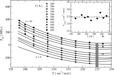
Figure 6: Inherent structures pressure, $P_{IS}$, as a function of $V$, for several isotherms. Each curve has been shifted by $n\times 30$ MPa, for a more clear presentation. Solid lines are the theoretical predictions according to the potential energy landscape equation of state of Ref. lanave . The shadowed region marks the range of variability of $V_{Sastry}$, the limit of stability for the inherent structures. Inset: $V_{Sastry}$ as a function of temperature for all the studied volumes is shown. Dashed line is the average value $224.9$ cm³/mol.

The previous observation stands out more clearly in Fig. 4 where the volume dependence of $P$, $P_{IS}$ and $P_{vib}$ is shown for the isotherm $T=320$ K. The total pressure $P$ is monotonically decreasing, confirming that the studied system is in the stable liquid phase up to $V=225$ cm³/mol. The IS pressure shows instead a minimum around $V=222$ cm³/mol, suggesting that, during the minimization process, a small cavity has been created in the $V=225$ cm³/mol sample. As a result, the significant drop observed at $V=225$ cm³/mol in $P_{vib}$ is an artifact induced by cavitation. It is also worth noting that a small decrease of $P_{vib}$ is observed already at $V=222$ cm³/mol, suggesting that the cavitation phenomenon is preceded by a weak softening of the vibrational density of states on approaching the Sastry instability.

Figure 7: Spinodal (open squares) and Kauzmann (open circles) lines, together with their extrapolations (dashed lines) in the $(T,V)$ plane. The relation between these two curves is discussed in the text. The vertical dashed line marks the Sastry volume, the limit of stability for the inherent structures. Some iso-entropic lines are also shown.

VII Limits of stability of the liquid

We now focus on the limits of stability of the liquid state. Fig. 5 shows the volume dependence of the pressure for several of the studied isotherms. Cavitation marks the homogeneous nucleation limit for the system; it can be detected during the simulation by monitoring the time dependence of pressure and potential energy, which show a clear discontinuity when a gas bubble nucleates. After the cavitation, $P$ increases and the potential energy decreases. We define the locus of homogeneous nucleation as the largest volume, at fixed $T$, at which we managed to simulate the dynamics of a homogeneous system. The fine grid of studied $V$ values allows us to identify such locus with a significant precision (solid line). Although the calculated homogeneous nucleation line refers to a system composed of $343$ molecules, it provides an upper bound for larger systems.

From the equilibrium $P(T,V)$ data, i.e., in the range where no cavitation is observed, it is possible to estimate the volume at which $P(V)$ has a minimum, by fitting the data according to the equation $P\approx(V-V_{s})^{2}$. In the mean field approximation, $V_{s}$ corresponds to the spinodal volume, and the temperature dependence of $V_{s}$ defines the spinodal locus (dashed line).

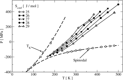
Figure 8: Spinodal (open squares) and Kauzmann (open circles) lines, together with their extrapolations (dashed lines) in the $(P,T)$ plane. The vertical dashed line marks the Sastry volume. Some iso-entropic lines are also shown.

We now focus on the information on liquid stability encoded in the inherent structures pressure $P_{IS}$. Fig. 6 shows, for several isotherms, $P_{IS}$ as a function of $V$. In analogy with the equilibrium data, a limit of stability for the inherent structures can be calculated estimating the minimum of $P_{IS}\approx(V-V_{Sastry})^{2}$ (fits are solid lines). It has been speculated that $V_{Sastry}$ represent the upper limit for glass formation, and that it may be identified with the $T\rightarrow 0$ limit of the liquid-gas spinodal locus sripre . Our calculations show that, as previously observed for other systems sriprl , the Sastry volume does not depend significantly on the temperature (see inset in Fig. 6).

We note that the Sastry volume is significantly smaller than the spinodal volume. The fact that $V_{Sastry}<V_{s}$ implies a stabilizing role of the vibrational component of the pressure. Indeed, already in Fig. 4 it was shown that the stability region for $P$ is larger than the one for $P_{IS}$. This fact suggests that, close to the spinodal line, the vibrational component becomes volume dependent to compensate for the loss of stability arising from the $P_{IS}$ contribution. Clearly, if $P_{vib}$ were $V$ independent, then $V_{s}$ and $V_{Sastry}$ should coincide. There is also an interesting observation to make concerning the application of the potential energy landscape approach to liquids at large volumes. Indeed, between $V_{Sastry}$ and $V_{s}$, the constant volume minimization procedure produces an inhomogeneous IS configuration notasastry . When the inherent structure contains voids, the determination of the landscape parameters proposed in this work becomes meaningless, and the link between the inherent structure and the corresponding liquid state requires a more detailed modeling.

Next, we focus on the location of the relevant stability loci of the liquid phase under supercooling. Within the Gaussian landscape model, the limit of stability of the supercooled liquid is defined by the line at which the configurational entropy vanishes, the so-called Kauzmann locus (Eq. (9)). As the spinodal curve is preempted by the homogeneous nucleation and, therefore, can not be approached in equilibrium, the Kauzmann locus can not be accessed due to the extremely slow structural relaxation times close to it. Still, these two loci provide a characterization of the domain of stability of the liquid state, and retain some meaning in a limiting mean-field sense.

Figs. 7 and 8 show the $S_{conf}=0$ locus and the spinodal locus in the $(T,V)$ and $(P,T)$ planes. The $(P,T)$ data have been calculated using the potential energy landscape equation of state introduced in Ref. lanave . Fig. 7 also shows curves at constant configurational entropy, in the region where no extrapolations are required. In analogy with the findings in Lennard Jones systems sriprl , the volume where the two loci appear to meet is close to $V_{Sastry}$, but at a temperature $T_{I}\simeq 73K$ different from $T=0$. Hence, the spinodal line terminates at a finite temperature, by merging with the $S_{conf}=0$ line; this is at odds with what was suggested in Ref. sripre . For $T_{I}\simeq 73K$, the glass will meet a mechanical instability on stretching; it is an interesting topic of research angelljcp ; angellprb ; sriprl to understand the relations between the volume at which such instability takes place and $V_{Sastry}$.

A recent thermodynamic analysis addresses the issue of the relative location of the two loci and the way these two loci intersect speedypisa ; speedypreprint . It has been suggested that the two lines must meet in $(P,T)$ plane with the same slope. Making use of the equation of state of Ref. lanave , the $(T,V)$ data of Fig. 7 can be represented in the $(P,T)$ plane. The phase diagram in $(P,T)$ is shown in Fig. 8, where also $T_{K}(P)$, the spinodal line and some iso-entropy curves are shown. An extrapolation of the low pressure behavior of the spinodal line shows that data are consistent with the possibility that the two lines meet with the same slope. If the pressure $P(T)$ along the spinodal increases with $T$, as usually found in liquids, the meeting point defines the lowest temperature and pressure that can be reached by the liquid in equilibrium. These values are $T_{I}\simeq 73$ K and $P_{I}\simeq=-360$ MPa.

VIII Summary and conclusions

In summary, we have studied the stability domain of the liquid state for a simple molecular model for ortho-terphenyl. In particular, we have focused on the two limits of stability, one provided by the divergence of the structural relaxation times, the other one provided by the cavitation of the gas phase. Both of them have theoretical mean-field bounds, the locus at which the configurational entropy vanishes and the locus at which the compressibility diverges, respectively.

To evaluate the configurational entropy, we have developed, along the lines of previous work for the same model otplungo , a potential energy landscape description of the system free energy, in the framework of the inherent structure thermodynamic formalism stillingerpes . The landscape analysis has required the evaluation of the statistical properties of the landscape, which we have quantified in the volume dependence of total number, energy distribution, and relation between energy depth and shape of the potential energy landscape basins.

The landscape analysis performed here is limited to volumes such that the minimization procedure, used for the evaluation of the inherent structures, results in an homogeneous structure. We have found that for volumes larger than the so-called Sastry density debenlewis ($V_{Sastry}\simeq 225$ cm³/mol) the system always cavitates upon minimization. Cavitation prevents the possibility of estimating the statistical properties of the landscape for $V\geq V_{Sastry}$. This poses a serious problem to the application of landscape approaches in the version where minimizations are performed at constant $V$ if the region close to the spinodal curve has to be investigated. Indeed, as shown in Fig. 7, the region of stability of the liquid phase extends well beyond $V_{Sastry}$. This suggests also that the region close to the spinodal curve is stabilized by vibrational contributions, which must overcome the destabilizing contribution arising from the configurational degrees of freedom (as discussed in Sec. VI). The stabilization in the vibrational properties appears to be accomplished by a softening of the vibrational density of states on approaching $V_{Sastry}$. We note on passing that, while in the $(T,V)$ ensemble, estimates of the liquid free energy in the IS formalism are limited to $V<V_{Sastry}$, formulations of the IS formalism in the $(P,T)$ ensemble does not suffer from such limitation, since the minimization path would not meet any instability curve.

In the framework of the IS formalism, we have estimated the locus at which configurational entropy vanishes. The possibility of a finite $T$ at which $S_{conf}$ vanishes is encoded in the model selected to represent the data. For all densities and temperatures studied in the present work, the Gaussian landscape heuer00 well represents the data and provides a well defined Kauzmann locus, whose location in the phase diagram has been compared with the location of the spinodal line. We have shown that the spinodal and the $S_{conf}=0$ loci may be extrapolated to meet at $V_{Sastry}$ at a finite $T$. Data are also consistent with the possibility that, in the $(P,T)$ plane, the two curves are tangent at $V_{Sastry}$. These two observations are in agreement with the behavior recently predicted for hard and soft spheres complemented by a mean field attraction. It will be interesting to address in the future the relation between the field of stability of the liquid as compared to the field of stability of the glass state.