A Stochastic Theory of Single Molecule Spectroscopy

Abstract

A theory is formulated for time dependent fluctuations of the spectrum of a single molecule in a dynamic environment. In particular, we investigate the photon counting statistics of a single molecule undergoing a spectral diffusion process. Based on the stochastic optical Bloch equation, fluctuations are characterized by Mandel’s $Q$ parameter yielding the variance of number of emitted photons and the second order intensity correlation function, $g^{(2)}(t)$. Using a semi-classical approach and linear response theory, we show that the $Q$ parameter can be described by a three-time dipole correlation function. This approach generalizes the Wiener-Khintchine formula that gives the average number of fluorescent photons in terms of a one-time dipole correlation function. We classify the time ordering properties of the three-time dipole correlation function, and show that it can be represented by three different pulse shape functions similar to those used in the context of nonlinear spectroscopy. An exact solution is found for a single molecule whose absorption frequency undergoes a two state random telegraph process (i.e., the Kubo-Anderson sudden jump process.) Simple expressions are obtained from the exact solution in the slow and fast modulation regimes based on appropriate approximations for each case. In the slow modulation regime $Q$ can be large even in the long time limit, while in the fast modulation regime it becomes small.

I Introduction

In recent years, a new approach to condensed phase spectroscopy has emerged, that focuses on the spectral properties of a single molecule (SM) embedded in a condensed phasemoerner-prl-89 ; moerner-sci-99 ; orrit-prl-90 ; tamarat-jpca-00 . Thanks to experimental advances made in optics and microscopysmbook-96 , it is now possible to perform single molecule spectroscopy (SMS) in many different systems. Motivations for SMS arise from a fundamental point of view (e.g., the investigation of the field-matter interaction at the level of a SM, the verification of statistical assumptions made in ensemble spectroscopy, etc) and from the possibility of applications (e.g., the use of SMS as a probe for large biomolecules for which a SM is attached as a fluorescent marker).

In general, the spectral properties of each individual molecule vary from molecule to molecule due to differences in the local environments with which each SM is interactingambrose-nature-91 ; ambrose-jcp-91 ; zumbusch-prl-93 ; fleury-jlum-93 ; kozankiewicz-jcp-94 ; vacha-jcp-97 ; boiron-cp-99 ; naumov-prb-01 ; geva-jpcb-97 ; brown-jcp-98 ; barkai-prl-00 . With its unique ability to detect dynamical phenomena occurring at the level of an individual molecule surrounded by its local environment, SMS has uncovered the statistical distributions of microscopic quantities of the environment that are hidden in traditional ensemble averaged spectroscopy. In particular, a single molecule spectrum measured for a finite time necessarily “sees” the temporal fluctuations of the host environment that occur on timescales comparable to the measurement timescale, and therefore lead, in many cases, to a stochastically fluctuating single molecule spectrum. Time dependent fluctuation phenomena in SMS occur in many ways, such as spectral diffusionambrose-nature-91 ; ambrose-jcp-91 ; zumbusch-prl-93 ; fleury-jlum-93 ; boiron-cp-99 ; bach-prl-99 and fluorescence intermittencybernard-jcp-93 ; basche-nature-95 ; brouwer-prl-98 ; kuno-jcp-00 ; neuhauser-prl-00 ; shimizu-prb-01 . The physical mechanisms causing these fluctuation phenomena vary depending on the dynamical processes a SM is undergoing, including: triplet state dynamicsbernard-jcp-93 ; basche-nature-95 ; brouwer-prl-98 , energy transfer processesha-pnas-96 ; vandenbout-sci-97 ; yip-jpca-98 , exciton transfer processesbach-prl-99 , chemical reactionswang-prl-95 ; chernyak-jcp-99 ; berezhkovskii-jpc-00 ; xie-acr-96 ; jia-pnas-97 ; lu-sci-98 , conformational changesschenter-jpca-99 ; agmon-jpcb-00 ; cao-cpl-00 ; yang-jpcb-01 , rotational dynamicsha-prl-96 ; ha-prl-98 , and diffusion processesedman-jpca-00 . Thus SMS provides a unique microscopic tool to investigate the dynamical processes that a SM and its environment undergo during the measurement time.

One important process responsible for time–dependent fluctuations in SMS is spectral diffusion, i.e., perturbations or excitations in the environment of the SM produce random changes in the transition frequency of the SMambrose-nature-91 ; ambrose-jcp-91 ; zumbusch-prl-93 ; fleury-jlum-93 ; boiron-cp-99 ; bach-prl-99 ; reilly-prl-93 ; reilly1-jcp-94 ; zumofen-cpl-94 ; tanimura-jcp-98 ; osadko-jcp-00 , leading to a time–dependent spectrum. Spectral diffusion processes have been observed in various systems including dye molecules in a molecular crystalambrose-nature-91 ; ambrose-jcp-91 and in a low temperature glasszumbusch-prl-93 ; fleury-jlum-93 , quantum dotsempedocles-prl-96 , light harvesting systemsvanoijen-sci-99 ; bopp-pnas-97 , and dendrimershofkens-jacs-00 . Since the spectral diffusion process directly reflects both (i) the interaction between the SM and its environment and (ii) the local dynamics of the latter, careful analysis of the time–dependent fluctuations of SMS illuminates the interplay between various dynamical processes in the condensed phase. In this work we formulate a stochastic theory of SMS undergoing a spectral diffusion process. In particular, we address the issue of the counting statistics of emitted photons produced by a SM undergoing a spectral diffusion process. Our studies show how the fluctuations in SMS can be used to probe the dynamics of SM and its interaction with the excitations of the environment.

Previously, the photon counting statistics of an ensemble of molecules, studied by various methods, for example, the fluorescence correlation spectroscopyelson-biopolym-74 ; ehrenberg-cp-74 ; koppel-pra-74 ; qian-bpchem-90 ; chen-bpj-99 has proved useful for investigating dynamical processes of various systems. The photon statistics of a SM is clearly different from that of the ensemble of molecules due both to the absence of inhomogeneous broadening and to the correlation between fluorescence photons that exists only on the SM level. In some SMS experiments, the measurement time is limited due to photobleaching, where the emission of a SM is quenched suddenly because of various reasons, for example, reaction with oxygen. Thus it is not an easy task in general to collect a sufficient number of photon counts to have good statistics. However, many SM–host systems have been found to remain stable for long enough time to measure photon statisticsbrunel-prl-99 ; fleury-prl-00 ; lounis-nature-00 ; nonn-prl-00 ; edman-jpca-00 ; molski-cpl-00b ; novikov-jcp-01 . In view of these recent experimental activities, a theoretical investigation of the counting statistics of photons produced by single molecules, in particular when there is a spectral diffusion process is timely and important.

We will analyze the SM spectra and their fluctuations semiclassically using the stochastic Bloch equation in the limit of a weak laser field. The Kubo-Anderson sudden jump approachanderson-jpsj-54 ; kubo-jpsj-54 ; kubo-fluct-62 is used to describe the spectral diffusion process. For several decades this model has been a useful tool for understanding line shape phenomena, namely, of the average number of counts $\langle n\rangle$ per measurement time $T$, and has found many applications mostly in ensemble measurements, e.g., NMR,kubo-statphys2-91 and nonlinear spectroscopy.mukamel-nonlinear-95 More recently, it was applied to model SMS in low temperature glass systems in order to describe the static properties of line shapes geva-jpcb-97 ; brown-jcp-98 ; barkai-prl-00 ; barkai-jcp-00 and also to model the time dependent fluctuations of SMS. plakhotnik-prl-98 ; plakhotnik-jlum-99 ; plakhotnik-prb-99

Mandel’s $Q$ parameter quantitatively describes the deviation of the photon statistics from the Poissonian casesaleh-photoelec-78 ; mandel-optical-95 ,

$$Q={\langle n^{2}\rangle-\langle n\rangle^{2}\over\langle n\rangle}-1,$$ (1)

where $n$ is the random number of photon counts, and the average is taken over stochastic processes involved. In the case of Poisson counting statistics $Q=0$ while our semiclassical results show super-Poissonian behavior ($Q>0$) for a SM undergoing a spectral diffusion process. For short enough times, fluorescent photons emitted by a SM show anti-bunching phenomena ($-1<Q<0$), a sub-Poissonian nonclassical effectfleury-prl-00 ; lounis-nature-00 ; basche-prl-92 ; michler-nature-00 ; short-prl-83 ; schubert-prl-92 . Our semiclassical approach is valid when the number of photon counts is large. Further discussion of the validity of our approach is given in Section VIII.

One of the other useful quantities to characterize dynamical processes in SMS is the fluorescence intensity correlation function, also called the second–order correlation function, $g^{(2)}(t)$, defined bycohentann-atom-93 ; loudon-qlight-83

$$g^{(2)}(\tau)={\langle I(t+\tau)I(t)\rangle\over\langle I\rangle^{2}}.$$ (2)

This correlation function has been used to analyze dynamical processes involved in many SMS experimentsyip-jpca-98 ; zumbusch-prl-93 ; weston-jcp-98 ; osadko-jetp-98 ; osadko-jetp-99 . Here $I(t)$ is the random fluorescence intensity observed at time $t$. It is well known that for a stationary process there is a simple relation between $g^{(2)}(t)$ and $Q(T)$fleury-prl-00 ; short-prl-83 ; kim-pra-87

$$Q(T)={2\langle I\rangle\over T}\int_{0}^{T}{\rm d}t_{1}\int_{0}^{t_{1}}{\rm d}t_{2}g^{(2)}(t_{2})-\langle I\rangle T,$$ (3)

where $T$ is the measurement time.

The essential quantity in the present formulation is a three–time correlation function, $C_{3}\left(\tau_{1},\tau_{2},\tau_{3}\right)$, which is similar to the nonlinear response function investigated in the context of four wave mixing processesmukamel-nonlinear-95 . The three–time correlation function contains all the microscopic information relevant for the calculation of the lineshape fluctuations described by $Q$. It has appeared as well in a recent paper of Plakhotnikplakhotnik-prb-99 in the context of intensity–time–frequency–correlation technique. In the present work, important time ordering properties of this function are fully investigated, and an analytical expression for $Q$ is found. The relation between $C_{3}\left(\tau_{1},\tau_{2},\tau_{3}\right)$ and lineshape fluctuations described by $Q$ generalizes the Wiener–Khintchine theorem, that gives the relation between the one–time correlation function and the averaged lineshape.

The timescale of the bath fluctuations is an important issue in SMS. Bath fluctuations are typically characterized as being in either fast or slow modulation regimes (to be defined later)kubo-fluct-62 . If the bath is very slow a simple adiabatic approximation is made based on the steady state solution of time–independent Bloch equation. Several studies have considered this simple limit in the context of SMSzumbusch-prl-93 ; fleury-jlum-93 ; reilly-prl-93 ; reilly1-jcp-94 . From a theoretical and also experimental point of view it is interesting to go beyond the slow modulation case. In the fast modulation case it is shown that a factorization approximation for the three–time correlation function yields a simple limiting solution. In this limit the lineshape exhibits the well known behavior of motional narrowing (as timescale of the bath becomes short, the line is narrowed). By considering a simple spectral diffusion process, we show that $Q$ exhibits a more complicated behavior than the lineshape does. When the timescale of the bath dynamics goes to zero, we find Poissonian photon statistics. Our exact results can be evaluated for an arbitrary timescale of the bath and are shown to interpolate between the fast and slow modulation regimes.

This paper is organized as follows. In Sec. II.1, the stochastic Bloch equation is presented and a brief discussion of its physical interpretation is given, and in Sec. II.2 the prescription for the relation between the solution of the optical Bloch equation and the discrete photon counts is described. We briefly review several results on counting statistics, which will later clarify the meaning of some of our results. Section III presents simple simulation results of SM spectra in the presence of the spectral diffusion to demonstrate a generic physical situation to which the present theory is applicable. In Sec. IV, an important relationship between $Q$ and the three-time correlation function is found, and the general properties of the latter are investigated. An exact solution for a simple spectral diffusion process is found in Sec. V. In Sec. VI we analyze the exact solution in various limiting cases so that the physical meaning of our results becomes clear. Connection of the present theory to experiments is made in Sec. VII. In Sec. VIII we further discuss the validity of the present model in connection with other approaches. We conclude in Sec. IX. Many of the mathematical derivations are relegated to the Appendices.

II Theory

Our theory presented in this section consists of two parts; first, we model the time evolution of a SM in a dynamic environment by the stochastic optical Bloch equation, and second, we introduce the photon counting statistics of a SM by considering the shot noise process due to the discreteness of photons.

II.1 Stochastic Optical Bloch Equation

We assume a simple nondegenerate two level SM in an external classical laser field. The electronic excited state $|e\rangle$ is located at energy $\omega_{0}$ above the ground state $|g\rangle$. We consider the time–dependent SM Hamiltonian

$$H={1\over 2}\hbar\omega_{0}\sigma_{z}+\sum_{j=1}^{J}{1\over 2}\hbar\Delta\omega_{j}(t)\sigma_{z}-{\bf d}\cdot{\bf E}_{0}\cos\left(\omega_{L}t\right),$$ (4)

where $\sigma_{z}$ is the Pauli matrix. The second term reflects the effect of the fluctuation of the environment on the absorption frequency of the SM coupled to $J$ perturbers. The stochastic frequency shifts $\Delta\omega_{j}(t)$ (i. e. the spectral diffusion) are random functions whose properties will be specified later. The last term in Eq. (4) describes the interaction between the SM and the laser field (frequency $\omega_{L}$), where ${\bf d}\equiv{\bf d}_{eg}\sigma_{x}$ is the dipole operator with the real matrix element ${\bf d}_{eg}=\langle e|{\bf d}|g\rangle$. We assume that the molecule does not have any permanent dipole moment either in the ground or in the excited state, $\langle g|{\bf d}|g\rangle=\langle e|{\bf d}|e\rangle=0$.

In the limit of a weak external field the model Hamiltonian describes the well known Kubo–Anderson random frequency modulation process whose properties are specified by statistics of $\Delta\omega_{j}(t)$anderson-jpsj-54 ; kubo-jpsj-54 ; kubo-fluct-62 . When the fluctuating part of the optical frequency $\Delta\omega_{j}$ is a two state random telegraph process, the Hamiltonian describes a SM (or spin of type $A$) coupled to $J$ bath molecules(or spins of type $B$), these being two level systems. Under certain conditions this Hamiltonian describes a SM interacting with many two level systems in low temperature glasses that has been used to analyze SM lineshapesgeva-jpcb-97 ; brown-jcp-98 ; barkai-prl-00 ; barkai-jcp-00 ; plakhotnik-jlum-99 ; plakhotnik-prb-99 .

The molecule is described by $2\times 2$ density matrix $\rho$ whose elements are $\rho_{gg},\rho_{ee},\rho_{ge},$ and $\rho_{eg}$. Let us define

$$u \equiv {1\over 2}{(\rho_{ge}e^{-i\omega_{L}t}+\rho_{eg}e^{i\omega_{L}t})},$$ (5)

$$v \equiv {1\over 2i}{(\rho_{ge}e^{-i\omega_{L}t}-\rho_{eg}e^{i\omega_{L}t})},$$ (6)

$$w \equiv {1\over 2}{(\rho_{ee}-\rho_{gg})},$$ (7)

and note that from the normalization condition $\rho_{ee}+\rho_{gg}=1$, we have $\rho_{ee}=w+1/2$. By using Eq. (4) the stochastic Bloch equations in the rotating wave approximation are given byshore-josab-84 ; colmenares-theochem-97

$$\dot{u} = \delta_{L}(t)v-{\Gamma u\over 2},$$ (8)

$$\dot{v} = -\delta_{L}(t)u-{\Gamma v\over 2}-\Omega w,$$ (9)

$$\dot{w} = \Omega v-\Gamma w-{\Gamma\over 2}.$$ (10)

$1/\Gamma$ is the radiative lifetime of the molecule added phenomenologically to describe spontaneous emission, $\Omega=-{\bf d}_{eg}\cdot{\bf E}_{0}/\hbar$ is the Rabi frequency, and the detuning frequency is defined by

$$\delta_{L}(t) = \omega_{L}-\omega_{0}-\Delta\omega(t),$$ (11)

$$\Delta\omega(t) = \sum_{j=1}^{J}\Delta\omega_{j}(t).$$ (12)

Besides the natural relaxation process described by $\Gamma$, other $T_{1}$ and $T_{2}$ processes can easily be included in the present theory. $w$ represents half the difference between the populations of the state $|e\rangle$ and $|g\rangle$, while $u$ and $v$ give the mean value of the dipole moment ${\bf d}$,

$$\mbox{Tr}\left(\rho{\bf d}\right)=2{\bf d}_{ge}\left[u\cos\left(\omega_{L}t\right)-v\sin\left(\omega_{L}t\right)\right].$$ (13)

In recent studieslounis-prl-97 ; brunel-prl-98 it has been demonstrated that the deterministic two level optical Bloch equation approach captures the essential features of SMS in condensed phases, which further justifies our assumptions.

The physical interpretation of the optical Bloch equation in the absence of time–dependent fluctuations is well knownmukamel-nonlinear-95 ; cohentann-atom-93 . Now that the stochastic fluctuations are included in our theory we briefly discuss the additional assumptions needed for standard interpretation to hold. The time–dependent power absorbed by the SM due to work of the driving field is,

$${{\rm d}{\cal{W}}\over{\rm d}t}=\cos\left(\omega_{L}t\right){\bf E}_{0}\cdot{{\rm d}\over{\rm d}t}\mbox{Tr}\left(\rho{\bf d}\right).$$ (14)

As usual, additional averaging (denoted with overbar) of Eq. (14) over the optical period of the laser is made. This averaging process is clearly justified for an ensemble of molecules each being out of phase. For a SM, such an additional averaging is meaningful when the laser timescale, $1/\omega_{L}$, is much shorter than any other timescale in the problem (besides $1/\omega_{0}$, of course). By using Eq. (13) this means,

$$\overline{v\cos^{2}(\omega_{L}t)}\approx v\overline{\cos^{2}(\omega_{L}t)},$$ (15)

under the conditions $|\dot{u}(t)|\ll\omega_{L}|v(t)|$ etc, and hence we have

$${{\rm d}\overline{\cal{W}}\over{\rm d}t}\simeq\hbar\Omega\omega_{L}v(t).$$ (16)

The absorption photon current (unit 1/[time]) iscohentann-atom-93

$$I(t)={1\over\hbar\omega_{L}}{{\rm d}\overline{\cal{W}}\over{\rm d}t}=\Omega v(t).$$ (17)

Neglecting photon shot noise (soon to be considered), $\int_{0}^{T}I(t){\rm d}t$ has the meaning of the number of absorbed photons in the time interval $(0,T)$ (i.e., since $\int_{0}^{T}({{\rm d}\overline{\cal{W}}\over{\rm d}t}){\rm d}t$ is the total work and each photon carries energy $\hbar\omega_{L}$). By using Eqs. (8)–(10), we have

$$\dot{\rho}_{ee}=\Omega v-\Gamma\rho_{ee}.$$ (18)

In the steady state, $\dot{\rho}_{ee}=0$, we have $\Omega v=\Gamma\rho_{ee}$, and since $\Omega v$ has a meaning of absorbed photon current, $\Gamma\rho_{ee}$ has the meaning of photon emission current. For the stochastic Bloch equation, a steady photon flux is never reached; however, integrating Eq. (18) over the counting time interval $T$,

$$\left[\rho_{ee}(T)-\rho_{ee}(0)\right]+\Gamma\int_{0}^{T}\rho_{ee}(t^{\prime}){\rm d}t^{\prime}=\Omega\int_{0}^{T}v(t^{\prime}){\rm d}t^{\prime},$$ (19)

and using $|\rho_{ee}(T)-\rho_{ee}(0)|\leq 1$ we find for large $T$ that the absorption and emission photon counts are approximately equal,

$$\underbrace{\Gamma\int_{0}^{T}\rho_{ee}(t){\rm d}t}_{\mbox{emitted photons}}\simeq\underbrace{\int_{0}^{T}I(t){\rm d}t\mbox{,}}_{\mbox{absorbed photons}}$$ (20)

provided that $\int_{0}^{T}I(t){\rm d}t\gg 1$. Eq. (20) is a necessary condition for the present theory to hold, and it means that the large number of absorbed photons is approximately equal to the large number of emitted photons (i. e. we have neglected any non–radiative decay channels). When there are non–radiative decay channels involved, one may modify Eq. (20) approximately by taking into account the fluorescence quantum yield, $\phi$, the ratio of the number of emitted photons to the number of absorbed photons,

$$\Gamma\int_{0}^{T}\rho_{ee}(t){\rm d}t\simeq\phi\int_{0}^{T}I(t){\rm d}t.$$ (21)

II.2 Classical Shot Noise

Time dependent fluctuations are produced not only by the fluctuating environment in SMS. In addition, an important source of fluctuations is the discreteness of the photon, i.e., shot noise. Assuming a classical photon emission process, the probability of having a single photon emission event in time interval $(t,t+{\rm d}t)$ ismandel-optical-95

$$\mbox{Prob}(t,t+{\rm d}t)=\Gamma\rho_{ee}(t){\rm d}t.$$ (22)

While this equation is certainly valid for ensemble of molecules all subjected to a hypothetical identical time–dependent environment, the validity of this equation for a SM is far from being obvious. In fact, as we discuss below, only under certain conditions we can expect this equation to be valid. By using Eq. (22) the probability of recording $n$ photons in time interval $(0,T)$ is given by the classical counting formulamandel-optical-95

$$p(n,T)={W^{n}\over n!}\exp\left(-W\right),$$ (23)

with

$$W=\eta\int_{0}^{T}I(t){\rm d}t,$$ (24)

where $\eta$ is a suitable constant depending on the detection efficiency. For simplicity we set $\eta=1$ here, but will re-introduce it later in our final expressions. Here $W=\eta\overline{\cal{W}}/\hbar\omega_{L}$ is $\eta$ times the work done by the driving laser field whose frequency is $\omega_{L}$ divided by the energy of one photon $\hbar\omega_{L}$ [see Eq. (17)]. It is a dimensionless time–dependent random variable, described by a probability density function $P(W,T)$, which at least in principle can be evaluated based on the statistical properties of the spectral diffusion process and the stochastic Bloch equations. From Eq. (23) and for a specific realization of the stochastic process $\Delta\omega(t)$, the averaged number of photons counted in time interval $(0,T)$ is given by $W$,

$$\langle n\rangle_{s}=\sum_{n=0}^{\infty}np(n,T)=W,$$ (25)

where the shot noise average is $\langle...\rangle_{s}=\sum_{n=0}^{\infty}...p(n,T)$. Since $W$ is random, additional averaging over the stochastic process $\Delta\omega(t)$ is necessary and statistical properties of the photon count are determined by $\langle p(n,T)\rangle$, where $\langle\cdots\rangle$ denotes averaging with respect to the spectral diffusion (i.e., not including the shot noise),

$$\langle p(n,T)\rangle=\left\langle{W^{n}\over n!}\exp(-W)\right\rangle.$$ (26)

Generally the calculation of $\langle p(n,T)\rangle$ is nontrivial; however, in some cases simple behavior can be found. Assuming temporal fluctuations of $W$ occur on the timescale $\tau_{c}$, then we have

(a) for counting intervals $T\gg\tau_{c}$ and for ergodic systems,

$$\lim_{T\to\infty}{\langle W\rangle\over T}=\lim_{T\to\infty}{1\over T}\int_{0}^{T}I(t){\rm d}t\equiv\langle I\left(\omega_{L}\right)\rangle,$$ (27)

which is the fluorescence lineshape of the molecule, that is, the averaged number of photon counts per unit time when the excitation laser frequency is $\omega_{L}$ [later we suppress $\omega_{L}$ in $\langle I\left(\omega_{L}\right)\rangle$]. Several authorschen-bpj-99 ; mandel-optical-95 ; schenzle-pra-86 have argued quite generally (though not in the SM context) that in the long measurement time limit we may use the approximation $W\simeq\langle I\rangle T$ (i.e., neglect the fluctuations), and hence photon statistics becomes Poissonianmandel-optical-95 ,

$$\langle p(n,T)\rangle\simeq{(\langle I\rangle T)^{n}\over n!}\exp(-\langle I\rangle T).$$ (28)

At least in principle $\langle I\rangle$ can be calculated based on standard lineshape theories, (e.g., in Appendix A we calculate $\langle I\rangle$ for our working example considered in Section V). Eq. (28) implies that a single measurement of the lineshape (i.e., averaged number of emitted photons as a function of laser frequency) determines the statistics of the photon count in the limit of long measurement time. In fact, it tells us that in this case, counting statistics beyond the average will not reveal any new information on the SM interacting with its dynamical environment. Mathematically this means that the distribution $P(W,T)$ satisfying

$$\langle p(n,T)\rangle=\int_{0}^{\infty}{\rm d}WP(W,T){W^{n}\over n!}\exp\left(-W\right)$$ (29)

converges to

$$P(W,T)\rightarrow\delta\left(W-\langle I\rangle T\right),$$ (30)

when $T\to\infty$. We argue below, however, using the central limit theorem, for cases relevant for SMS, $P(W,T)$ is better described by a Gaussian distribution. The transformation Eq. (29) is called the Poisson transform of $P(W,T)$saleh-photoelec-78 .

(b) in the opposite limit, $T\ll\tau_{c}$ we may use the approximationwalls-quantopt

$$W\simeq I_{0}T,$$ (31)

where $I_{0}=I(T=0)$. In a steady state $\langle p(n,T)\rangle$ can be calculated if the distribution of intensity (i.e., photon current) is known

$$\langle p(n,T)\rangle\simeq\int_{0}^{\infty}{\rm d}I_{0}P(I_{0})e^{-I_{0}T}{\left(I_{0}T\right)^{n}\over n!}.$$ (32)

For example, assume that $I(t)$ is a two state process, i. e. the case when a SM is coupled to a single slow two level system in a glass, then

$$P(I)=p_{1}\delta\left(I-I_{1}\right)+p_{2}\delta\left(I-I_{2}\right),$$ (33)

and

$$\langle p(n,T)\rangle=\sum_{i=1,2}p_{i}{\left(I_{i}T\right)^{n}\over n!}\exp\left(-I_{i}T\right),$$ (34)

and if, for example, $I_{2}\sim 0$, the SM is either “on” or “off”, a case encountered in several experimentslu-sci-98 ; empedocles-prl-96 ; xie-acr-96 .

(c) a more challenging case is when $T\simeq\tau_{c}$; later, we address this case in some detail.

We would like to emphasize that the photon statistics we consider is classical, while the Bloch equation describing dynamics of the SM has quantum mechanical elements in it (i.e., the coherence). In the weak laser intensity case the Bloch equation approach allows a classical interpretation based on the Lorentz oscillator model as presented in Appendix B.

III Simulation

To illustrate combined effects of the spectral diffusion and the shot noise on the fluorescence spectra of a SM, we present simulation results of spectral trails of a SM, where the fluorescence intensity of a SM is measured as a function of the laser frequency as the spectral diffusion proceedsboiron-cp-99 ; ambrose-jcp-91 .

First, we present a simple algorithm for generating random fluorescence based on the theory presented in Section II, by using the stochastic Bloch equation, Eqs. (8)-(10), and the classical photon counting distribution, Eq. (23). A measurement of the spectral trail is performed from $t=0$ to $t=t_{\rm end}$. As in the experimental situation, we divide $t_{\rm end}$ into $N$ time bins each of which has a length of time $T$. For each bin time $T$, a random number of photon counts is recorded. Simulations are performed following the steps described below:

Step (1) Generate a spectral diffusion process $\Delta\omega(t)$ from $t=0$ to $t=t_{{\rm end}}$.

Step (2) Solve the stochastic Bloch equation, Eqs. (8)-(10), for a random realization of the spectral diffusion process generated in Step ($1$) for a given value of $\omega_{L}$ during the time period $0<t<t_{\rm{end}}$.

Step (3) Determine $W(t_{k},\omega_{L})$ during the $k$th time bin ($k=1,2,3,\cdots N$), $(k-1)T<t<kT$, with a measurement time $T$ according to Eq. (24),

$$W(t_{k},\omega_{L})=\int_{(k-1)T}^{kT}{\rm d}tI(t).$$ (35)

Step (4) Generate a random number $0<x<1$ using a uniform random number generator, and then the random count $n$ is found using the criterion,

$$\sum_{j=0}^{n-1}p\left(j,W\right)<x\leq\sum_{j=0}^{n}p\left(j,W\right).$$ (36)

According to Eq. (23) we find

$${\Gamma\left(n,W\right)\over\left(n-1\right)!}<x\leq{\Gamma\left(n+1,W\right)\over n!},$$ (37)

where $\Gamma(a,z)$ is the incomplete gamma function. Steps ($1-4$) must be repeated many times to get good statistics.

For an illustration purpose we choose a simple model of the spectral diffusion, which is called a two state jump process or a dichotomic process. We assume that the frequency modulation can be either $\Delta\omega(t)=\nu$ or $\Delta\omega(t)=-\nu$, and the flipping rate between these two frequency modulations is given by $R$. This model will be used as a working example for which an analytical solution is obtained later in Section V.

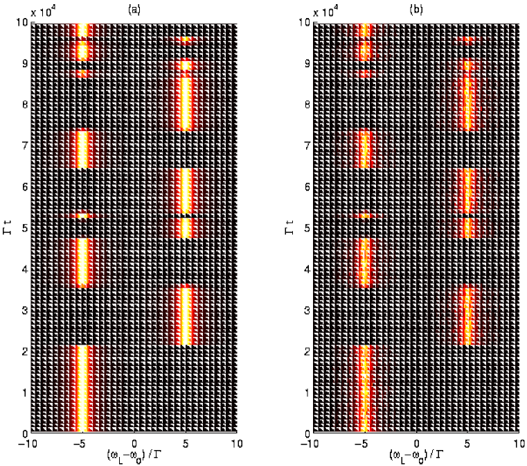
Figure 1: Spectral trails of a SM undergoing a very slow spectral diffusion process described by the two state jump model are shown for (a) $W$ (without the shot noise) and (b) $n$ (with the shot noise). Parameters are chosen as $\Omega=0.2\Gamma$, $R=10^{-4}\Gamma$, $\nu=5\Gamma$, $T=10^{3}\Gamma^{-1}$, $t_{\rm end}=10^{5}\Gamma^{-1}=100T$, and $\Gamma=1$.

In Fig. 1 we present a simulation result of one realization of a spectral diffusion process when the fluctuation rate $R$ is much smaller than $\Gamma$ and $\nu$ (slow modulation regime to be defined later). Parameters are given in the figure caption. Fig. 1(a) shows $W(t_{k},\omega_{L})$, demonstrating the effects of the spectral diffusion process on the fluorescence spectra. Note that $W(t_{k},\omega_{L})$ has been defined without the shot noise. One can clearly see that the resonance frequency of a SM is jumping between two values as time goes on, and $W$ shows its maximum values either at $\omega_{L}-\omega_{0}=\nu$ or at $\omega_{L}-\omega_{0}=-\nu$. Since shot noise is not considered in Fig. 1(a), $W$ appears smooth and regular between the flipping events. In Fig. 1(b) we have taken into account the effects of shot noise as described in Step ($4$) and plotted the random counts $n$ as a function of $\omega_{L}$ and $t$. Compared to Fig. 1(a), the spectral trail shown in Fig. 1(b) appears more fuzzy and noisy due to the shot noise effect. It looks similar to the experimentally observed spectral trails (see, for example, Ref. boiron-cp-99 ).

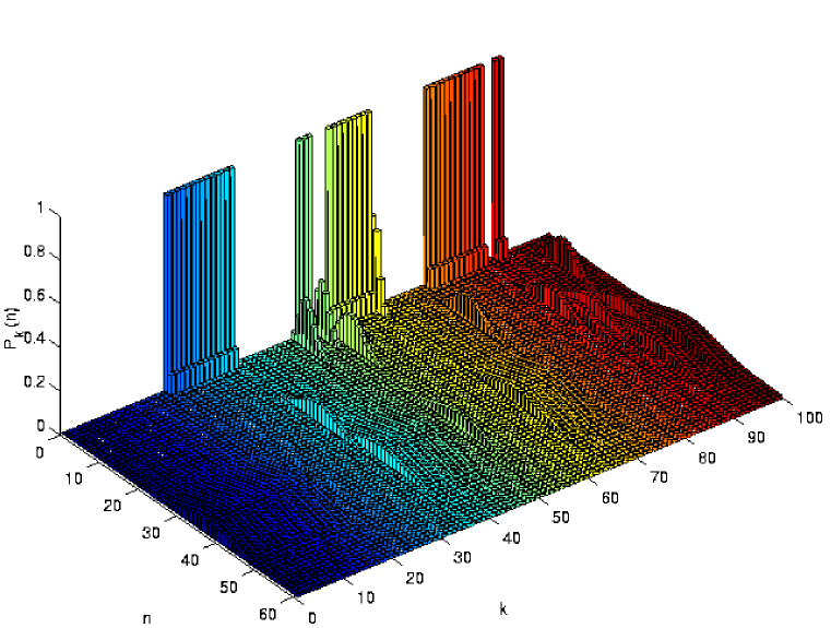
Figure 2: Time evolution of photon counting distributions $P_{k}(n)$ for the slow modulation case corresponding to $\omega_{L}-\omega_{0}=-\nu$ in Fig. 1. Other parameters are given in Fig. 1.

In Fig. 2 we show the evolution of the photon counting distribution $P_{k}(n)$, Eq. (23), at a fixed laser frequency, chosen here as $\omega_{L}-\omega_{0}=-\nu=-5\Gamma$. The spectral diffusion process is identical to that shown in Fig. 1. Here $k$ denotes the measurement performed during the $k$th time bin as described in Step ($3$). Notice that two distinct forms of the photon counting distributions appear. During the dark period at the chosen frequency $\omega_{L}-\omega_{0}=-\nu$ in Fig. 1 (e.g., $2.1\times 10^{4}<\Gamma t<3.5\times 10^{4}$ corresponding to $21<k<35$), $P_{k}(n)$ reaches its maximum at $n=0$ with $P_{k}(n=0)\simeq 1$ and $P_{k}(n>1)\ll 1$, meaning that the probability for a SM not to emit any photon during each time bin in the dark period is almost one. However, during the bright period (for example, $3.5\times 10^{4}<\Gamma t<4.6\times 10^{4}$ corresponding to $35<k<46$), $P_{k}(n)$ shows a wide distribution with $\langle n\rangle_{s}\simeq 35$, meaning that on the average $\langle n\rangle_{s}\simeq 35$ number of photons are emitted per bin during this period. As the spectral diffusion proceeds, one can see the corresponding changes in the photon counting distribution, $P_{k}(n)$, typically among these two characteristic forms.

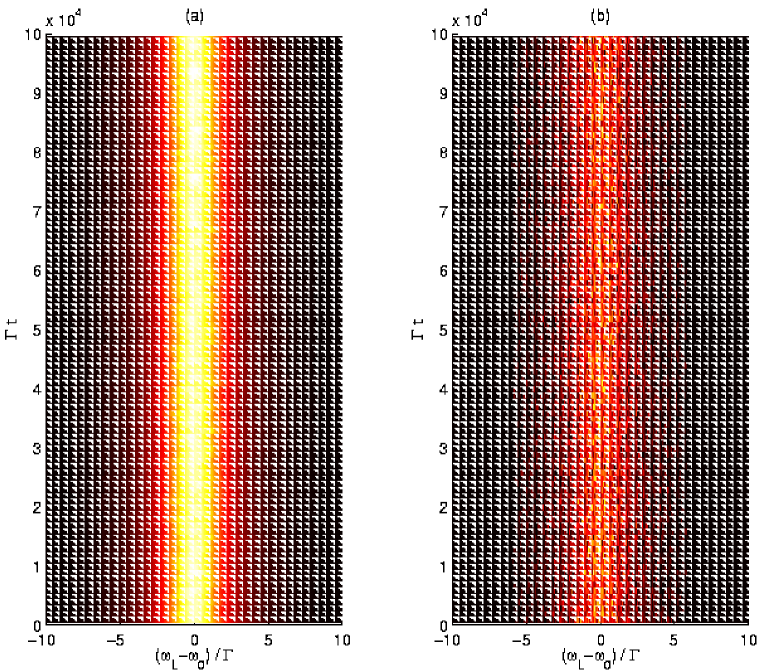
Figure 3: Spectral trails of a SM undergoing a fast spectral diffusion process described by the two state jump model are shown for (a) $W$ (without the shot noise) and (b) $n$ (with the shot noise). Parameters are chosen as $\Omega=0.2\Gamma$, $R=10\Gamma$, $\nu=5\Gamma$, $T=10^{3}\Gamma^{-1}$, $t_{\rm end}=10^{5}\Gamma^{-1}=100T$, and $\Gamma=1$.

In Fig. 3 we present a simulation result of a spectral trail for the case when the resonance frequency of a SM fluctuates very quickly compared with $\Gamma$ and $\nu$ (i. e.  $R\gg\nu\gg\Gamma$). In this case, since the frequency modulation is so fast compared with the spontaneous emission rate, a large number of frequency modulations are realized during the time $1/\Gamma$, and the frequency of the SM where the maximum photon counts are observed is dynamically averaged between $\omega_{0}-\nu$ and $\omega_{0}+\nu$ (i. e. a motional narrowing phenomenon)kubo-fluct-62 ; talon-josab-92 . The width of the spectral trail is approximately $\Gamma$, and no splitting is observed even though the frequency modulation $\nu$ is larger than the spontaneous decay rate $\Gamma$ ($\nu=5\Gamma$ in this case). This behavior is very different from the slow modulation case shown in Fig. 1, where two separate trails appear at $\omega_{L}=\omega_{0}\pm\nu$.

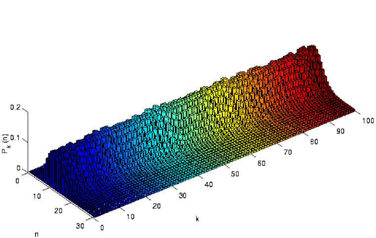
Figure 4: Time evolution of photon counting distributions $P_{k}(n)$ for the fast modulation case corresponding to $\omega_{L}=\omega_{0}$ in Fig. 3. Other parameters are given in Fig. 3.

In Fig. 4 we also show the evolution of the photon counting distribution $P_{k}(n)$ during a spectral diffusion process at a fixed frequency $\omega_{L}=\omega_{0}$ where the lineshape reaches its maximum in the fast fluctuation case shown in Fig. 3. Unlike the slow modulation case in Fig. 2, where one can see large fluctuations of the photon counting distributions, the fluctuations of the photon counting distributions are much smaller in the fast modulation case, and $P_{k}(n)$ shows a broad Gaussian-like behavior, centered at $\langle n\rangle_{s}\simeq 12$.

IV $Q$ and Three–Time Correlation Function

Having observed the interplay between spectral diffusion and shot noise on the fluorescence spectra of a SM in simple simulation results of the previous section, it is natural to ask how one can analyze theoretically the photon counting statistics of a SM in the presence of a spectral diffusion process. The probability density of the number of photon counts $\langle p(n,T)\rangle$, or equivalently $P(W,T)$ in Eq. (29), would give complete information of the dynamical processes of a SM undergoing a spectral diffusion process, but is difficult to calculate in general. In order to obtain dynamical information, we will consider the mean $\langle W\rangle$ and the second moment $\langle W^{2}\rangle$ of the random photon counts.

It is easy to show that the average number of photons counted in time interval $(0,T)$ is given from Eq. (26),

$$\langle\langle n\rangle_{s}\rangle=\sum_{n=0}^{\infty}n\langle p(n,T)\rangle=\langle W\rangle,$$ (38)

and the second factorial moment of the photon counts in time interval $(0,T)$ is given by

$$\langle\langle n(n-1)\rangle_{s}\rangle=\sum_{n=0}^{\infty}n(n-1)\langle p(n,T)\rangle=\langle W^{2}\rangle.$$ (39)

The Mandel $Q$ parameter is now introduced to characterize the fluctuationsmandel-optical-95 ,

$${\langle\langle n^{2}\rangle_{s}\rangle-\langle\langle n\rangle_{s}\rangle^{2}\over\langle\langle n\rangle_{s}\rangle}=1+Q,$$ (40)

and it is straightforward to show thatmandel-optical-95

$$Q={\langle W^{2}\rangle-\langle W\rangle^{2}\over\langle W\rangle}.$$ (41)

This equation is important relating $Q$ to the variance of the stochastic variable $W$. We see that $Q\geq 0$, indicating that photon statistics is super-Poissonian. For our classical case we anticipate:
(a) for an ergodic system, when $T/\tau_{c}\to\infty$, and if Eq. (28) is strictly valid, $Q\to 0$ (i.e., Poissonian statistics). However, below we find an analytical expression for $Q$ which is non–zero and in some cases large even in the limit of $T\to\infty$. We will discuss this subtle issue later;
(b) in the opposite limit, $T\ll\tau_{c}$,

$$Q={\langle I_{0}^{2}\rangle-\langle I_{0}\rangle^{2}\over\langle I_{0}\rangle}T;$$ (42)

(c) if $I(t)=I$, independent of time, $Q=0$, as expected;
(d) it is easy to see that $Q\propto\eta$, hence when $\eta\to 0$, counts recorded in the measuring device tend to follow the Poissonian counting statistics.

We now consider the important limit of weak laser intensity. In this limit the Wiener–Khintchine theorem relating the lineshape to the one–time correlation function holds. As we shall show now, a three–time correlation function is the central ingredient of the theory of fluctuations of SMS in this limit. In Appendix B we perform a straightforward perturbation expansion with respect to the Rabi frequency $\Omega$ in the Bloch equation, Eqs. (8)-(10), to find

$$v\left(t\right)={\Omega\over 2}\mbox{Re}\left\{\int_{0}^{t}{\rm d}t_{1}\exp\left[-i\int_{t_{1}}^{t}{\rm d}t^{\prime}\delta_{L}(t^{\prime})-{\Gamma\over 2}(t-t_{1})\right]\right\}.$$ (43)

According to the discussion in Section II the random number of photons absorbed in time interval $(0,T)$ is determined by $W=\Omega\int_{0}^{T}v(t){\rm d}t$ (see Eqs. (17) and (24)), and from Eq. (43) we find

$$W={\Omega^{2}\over 2}\mbox{Re}\left[\int_{0}^{T}{\rm d}t_{2}\int_{0}^{t_{2}}{\rm d}t_{1}e^{-i\omega_{L}(t_{2}-t_{1})-\Gamma(t_{2}-t_{1})/2+i\int_{t_{1}}^{t_{2}}{\rm d}t^{\prime}\Delta\omega(t^{\prime})}\right],$$ (44)

where we have neglected terms of higher order than $\Omega^{2}$. In standard lineshape theories Eq. (44) is averaged over the stationary stochastic process and the long time limit is taken, leading to the well known result for the (unnormalized) lineshape

$$\langle I(\omega_{L})\rangle=\lim_{T\to\infty}{\langle W\rangle\over T}={\Omega^{2}\over 2}\mbox{Re}\left[\int_{0}^{\infty}{\rm d}\tau e^{-i\omega_{L}\tau-\Gamma\tau/2}C_{1}^{-1}\left(\tau\right)\right],$$ (45)

where we have set $\omega_{0}=0$. The one–time correlation function $C_{1}^{l}(\tau)$ is defined by

$$C_{1}^{l}(\tau)=\langle e^{-il\int_{0}^{\tau}\Delta\omega(t^{\prime}){\rm d}t^{\prime}}\rangle,$$ (46)

where $l=\pm 1$ and $\langle\cdots\rangle$ is an average over the stochastic trajectory $\Delta\omega$. Eq. (45) is the celebrated Wiener–Khintchine formula relating the one–time correlation function to the average number of photon counts, i. e. the averaged lineshape of a SM. We now investigate lineshape fluctuation by considering the statistical properties of $W$.

Using Eq. (43) we show in Appendix B that

$$\langle W^{2}\rangle={\Omega^{4}\over 16}\int_{0}^{T}\int_{0}^{T}\int_{0}^{T}\int_{0}^{T}{\rm d}t_{1}{\rm d}t_{2}{\rm d}t_{3}{\rm d}t_{4}e^{-i\omega_{L}(t_{2}-t_{1}+t_{3}-t_{4})-\Gamma(|t_{1}-t_{2}|+|t_{3}-t_{4}|)/2}$$

$$\mbox{\makebox[36.135pt]{ }}\times\left\langle\exp\left[i\int_{t_{1}}^{t_{2}}\Delta\omega(t^{\prime}){\rm d}t^{\prime}-i\int_{t_{3}}^{t_{4}}\Delta\omega(t^{\prime}){\rm d}t^{\prime}\right]\right\rangle.$$ (47)

As can be seen from Eq. (47) the key quantity of the theory of lineshape fluctuation is the three–time correlation function,

$$C_{3}\left(\tau_{1},\tau_{2},\tau_{3}\right)=\left\langle\exp\left[i\int_{t_{1}}^{t_{2}}\Delta\omega(t^{\prime}){\rm d}t^{\prime}-i\int_{t_{3}}^{t_{4}}\Delta\omega(t^{\prime}){\rm d}t^{\prime}\right]\right\rangle,$$ (48)

which depends on the time ordering of $t_{1},t_{2},t_{3},t_{4}$. In Eq. (48) we have defined the time ordered set of $\{t_{1},t_{2},t_{3},t_{4}\}$ as $\{t_{I},t_{II},t_{III},t_{IV}\}$ such that $t_{I}<t_{II}<t_{III}<t_{IV}$, and $\tau_{1}=t_{II}-t_{I}$, $\tau_{2}=t_{III}-t_{II}$ and $\tau_{3}=t_{IV}-t_{III}$. Due to the stationarity of the process $C_{3}\left(\tau_{1},\tau_{2},\tau_{3}\right)$ does not depend on the time elapsing between start of observation $t=0$ and $t_{I}$. It has a similar mathematical structure to that of the nonlinear response function used to describe four wave mixing spectroscopies such as photon echo or hole burningmukamel-nonlinear-95 .

$\ m\$	$S_{m}(t)$	$C_{3}^{m}(\tau_{1},\tau_{2},\tau_{3})$	time ordering
$\ 1\$		$\ {1\over 2}\sum P_{ij}^{-1}(\tau_{1})P_{jk}^{0}(\tau_{2})P_{kl}^{1}(\tau_{3})\$	$\ t_{1}<t_{2}<t_{3}<t_{4}\$
$\ 2\$		$\ {1\over 2}\sum P_{ij}^{1}(\tau_{1})P_{jk}^{0}(\tau_{2})P_{kl}^{-1}(\tau_{3})\$	$\ t_{2}<t_{1}<t_{4}<t_{3}\$
$\ 3\$		$\ {1\over 2}\sum P_{ij}^{1}(\tau_{1})P_{jk}^{0}(\tau_{2})P_{kl}^{1}(\tau_{3})\$	$\ t_{2}<t_{1}<t_{3}<t_{4}\$
$\ 4\$		$\ {1\over 2}\sum P_{ij}^{-1}(\tau_{1})P_{jk}^{0}(\tau_{2})P_{kl}^{-1}(\tau_{3})\$	$\ t_{1}<t_{2}<t_{4}<t_{3}\$
$\ 5\$		$\ {1\over 2}\sum P_{ij}^{1}(\tau_{1})P_{jk}^{2}(\tau_{2})P_{kl}^{1}(\tau_{3})\$	$\ t_{2}<t_{3}<t_{1}<t_{4}\$
$\ 6\$		$\ {1\over 2}\sum P_{ij}^{-1}(\tau_{1})P_{jk}^{-2}(\tau_{2})P_{kl}^{-1}(\tau_{3})\$	$\ t_{1}<t_{4}<t_{2}<t_{3}\$

Table 1: Three–time correlation functions $C_{3}^{m}$ represented by six different pulse shape functions $S_{m}(t)$ for $24$ time orderings schemes. Values of $S_{m}(t)$ for each time interval are shown to the left of the pulse shape. Only one representative time ordering scheme for each class is shown in the third column. Three other time ordering schemes belonging to the same class are obtained by exchanging $t_{1}\leftrightarrow t_{4}$ and/or $t_{2}\leftrightarrow t_{3}$. For example, three other time orderings belonging to $m=1$ are $t_{4}<t_{2}<t_{3}<t_{1}$, $t_{1}<t_{3}<t_{2}<t_{4}$, and $t_{4}<t_{3}<t_{2}<t_{1}$. In the second column expressions of the three–time correlation functions $C_{3}^{m}$ are shown in terms of the weight functions considered in Section V. Note that $C_{3}^{2n-1}(\tau_{1},\tau_{2},\tau_{3})$ and $C_{3}^{2n}(\tau_{1},\tau_{2},\tau_{3})$ $(n=1,2,3)$ are complex conjugates of each other.

In Eq. (48) there are $4!=24$ options for the time ordering of $(t_{1},t_{2},t_{3},t_{4})$; however, as we show below, only three of them (plus their complex conjugates) are needed. It is convenient to rewrite the three–time correlation function as a characteristic functional,

$$C_{3}^{m}\left(\tau_{1},\tau_{2},\tau_{3}\right)=\left\langle\exp\left[-i\int_{t_{I}}^{t_{IV}}S_{m}(t^{\prime})\Delta\omega(t^{\prime}){\rm d}t^{\prime}\right]\right\rangle,$$ (49)

where $S_{m}(t)$ ($m=1,2,\cdots,6$) is defined in Table 1 as the pulse shape function corresponding to the $m$th time ordering. Let us consider as an example the case $m=1$, $t_{1}<t_{2}<t_{3}<t_{4}$ (for which $t_{1}=t_{I},t_{2}=t_{II},\cdots$, and $\tau_{1}=t_{2}-t_{1}$, $\tau_{2}=t_{3}-t_{2}$, and $\tau_{3}=t_{4}-t_{3}$). Then the pulse shape function is given by

$$S_{1}(t)=\left\{\begin{array}[]{c c}-1&t_{I}<t<t_{II}\\ 0&t_{II}<t<t_{III}\\ 1&t_{III}<t<t_{IV},\end{array}\right.$$ (50)

and the shape of this pulse is shown in the first line of Table 1. Similarly, other pulse shapes describe the other time orderings.

The four dimensional integration in Eq. (47) is over $24$ time orderings. We note, however, that

$$e^{-i\omega_{L}(t_{2}-t_{1}+t_{3}-t_{4})-\Gamma(|t_{1}-t_{2}|+|t_{3}-t_{4}|)/2}\left\langle\exp\left[i\int_{t_{1}}^{t_{2}}{\rm d}t^{\prime}\Delta\omega(t^{\prime})-i\int_{t_{3}}^{t_{4}}{\rm d}t^{\prime}\Delta\omega(t^{\prime})\right]\right\rangle$$

in Eq. (47) has two important properties: (a) the expression is invariant when we replace $t_{1}$ with $t_{4}$ and $t_{2}$ with $t_{3}$, and (b) the replacement of $t_{1}$ with $t_{2}$ (or $t_{3}$) and of $t_{3}$ with $t_{4}$(or $t_{1}$) has a meaning of taking the complex conjugate. Hence it is easy to see that only three types of time orderings (plus their complex conjugates) must be considered. Each time ordering corresponds to different pulse shape function, $S_{m}(t)$. In Table 1, for all six time ordering schemes, the corresponding pulse shape functions are presented. We also give expressions of $C^{m}_{3}(t)$ for the working example to be considered soon in Section IV.

We note that if $\tau_{1}=\tau_{3}$ the pulse in Eq. (50) is identical to that in the three–time photon echo experiments. The important relation between lineshape fluctuations and nonlinear spectroscopy has been pointed out by Plakhotnik in Ref. plakhotnik-prb-99 in the context of intensity–time–frequency–correlation measurement technique.

V Two State Jump Model: Exact Solution

V.1 Model

In order to investigate basic properties of lineshape fluctuations we consider a simple situation. We assume that there is only one bath molecule that is coupled to a chromophore by setting $J=1$ and $\Delta\omega_{1}(t)=\nu h(t)$ in Eq. (4), where $\nu$ is the magnitude of the frequency shift and measures the interaction of the chromophore with the bath, and $h(t)$ describes a random telegraph process $h(t)=1$ or $h(t)=-1$ depending on the bath state, up or down, respectively. For simplicity, the transition rate from up to down and vice versa are assumed to be $R$. The generalization to the case of different up and down transition rates is important, but not considered here. A schematic representation of the spectral diffusion process is given in Fig. 5.

Figure 5: A schematic representation of the spectral diffusion process modeled by two state jump process(random telegraph noise). The fluctuating transition frequency is given by $\Delta\omega(t)=\nu h(t)$.

This model introduced by Kubo and Anderson in the context of stochastic lineshape theoryanderson-jpsj-54 ; kubo-jpsj-54 is called the sudden jump model, and it describes a stochastic process that describes fluctuation phenomena arising from Markovian transitions between discrete statesanderson-jpsj-54 ; kubo-jpsj-54 . For several decades the Kubo–Anderson sudden jump model has been a useful tool for understanding lineshape phenomena, namely, of the average number of counts $\langle n\rangle$ per measurement time $T$, and has found many applications mostly in ensemble measurements, e.g., NMRkubo-fluct-62 and nonlinear spectroscopymukamel-nonlinear-95 . More recently, it was applied to model SMS in low temperature glass systems in order to describe the static properties of lineshapesgeva-jpcb-97 ; brown-jcp-98 ; barkai-prl-00 and also to model the time–dependent fluctuations of SMSplakhotnik-prl-98 ; plakhotnik-jlum-99 ; plakhotnik-prb-99 . In this paper, we will consider this model as a working example to study properties of lineshape fluctuations.

The above model can describe a single molecule coupled to a single two level system in low temperature glasses as explained in Section VII. In this case $\nu$ depends on the distance between the SM and the two level systemesquinazi-tunn-98 . Another physical example of this model is the following: consider a chromophore that is attached to a macromolecule, and assume that conformational fluctuations exist between two conformations of the macromolecule. Depending on the conformation of the macromolecule, the transition frequency of the chromophore is either $\omega_{0}-\nu$ or $\omega_{0}+\nu$jia-pnas-97 .

V.2 Solution

By using a method of Suárez and Silbeysuarez-cpl-94 , developed in the context of photon echo experiments, we now analyze the properties of the three–time correlation function. We first define the weight functions,

$$P^{a}_{if}(t)=\left\langle\exp\left[-ia\int_{0}^{t}\Delta\omega(t^{\prime}){\rm d}t^{\prime}\right]\right\rangle_{if},$$ (51)

where the initial (final) state of the stochastic process $\Delta\omega$ is $i$ ($f$) and $a=0$ or $a=\pm 1$ or $a=\pm 2$. For example, $P^{-1}_{++}(t)$ is the value of $\langle e^{i\int_{0}^{t}\Delta\omega(t^{\prime}){\rm d}t^{\prime}}\rangle$ for a path restricted to have $\Delta\omega(0)=\nu$ and $\Delta\omega(t)=\nu$. The one–time correlation function $C_{1}^{l}(\tau)$ defined in Eq. (46) can be written as sum of these weights,

$$C_{1}^{l}\left(\tau\right)={1\over 2}\sum_{i,j}P_{ij}^{l}(\tau),$$ (52)

where a prefactor $1\over 2$ is due to the symmetric initial condition and the summation is over all the possible paths during time $\tau$(i. e. $i=\pm,j=\pm$). Also by using the Markovian property of the process, we can express all the $C_{3}^{m}$ functions in terms of the weights. For example, for the pulse shape in Eq. (50)

$$C_{3}^{1}\left(\tau_{1},\tau_{2},\tau_{3}\right)={1\over 2}\sum_{i,j,k,l}P^{-1}_{ij}\left(\tau_{1}\right)P^{0}_{jk}\left(\tau_{2}\right)P_{kl}^{1}\left(\tau_{3}\right),$$ (53)

where the summations are over all possible values of $i=\pm$, $j=\pm$, $k=\pm$, and $l=\pm$. The other $C_{3}^{m}$ functions are expressed in terms of weights in Table 1. Explicit expressions of the weights for the working model are given by

$$P_{if}^{0}(t) = {1\over 2}[1+(-1)^{\delta_{if}+1}\exp(-2Rt)],$$ (54)

$$P_{+-}^{1}(t) = P_{-+}^{1}(t)=R\exp(-Rt)\sin(Y_{1}t)/Y_{1},$$ (55)

$$P_{\pm\pm}^{1}(t) = \exp(-Rt)\left[\cos\left(Y_{1}t\right)\mp i\nu{\sin\left(Y_{1}t\right)\over Y_{1}}\right],$$ (56)

$P_{if}^{-1}(t)=\mbox{C.C.}\left[P_{if}^{1}\left(t\right)\right]$ where C.C. denotes complex conjugate, and $Y_{1}=\sqrt{\nu^{2}-R^{2}}$. $P^{\pm 2}_{if}(t)$ is given by the same expressions as the corresponding $P^{\pm 1}_{if}(t)$ with $\nu$ replaced by $2\nu$.

Now we can evaluate $\langle W\rangle$ and $\langle W^{2}\rangle$ explicitly. First we consider $\langle W^{2}\rangle$ and, in particular, focus on the case $m=1$, $0<t_{1}<t_{2}<t_{3}<t_{4}<T$. By using Table 1, the contribution of $\langle W^{2}\rangle$ to Eq. (47) is

$$\langle W^{2}\rangle_{1234}={\Omega^{4}\over 16}\int_{0}^{T}{\rm d}t_{4}\int_{0}^{t_{4}}{\rm d}t_{3}\int_{0}^{t_{3}}{\rm d}t_{2}\int_{0}^{t_{2}}{\rm d}t_{1}e^{-i\omega_{L}(t_{2}-t_{1}+t_{3}-t_{4})-\Gamma(|t_{1}-t_{2}|+|t_{3}-t_{4}|)/2}$$

$$\mbox{\makebox[57.81621pt]{ }}\times{1\over 2}\sum_{i,j,k,l}P_{ij}^{-1}(t_{2}-t_{1})P_{jk}^{0}(t_{3}-t_{2})P_{kl}^{1}(t_{4}-t_{3}).$$ (57)

We use the convolution theorem of Laplace transform four times and find

$$\langle W^{2}\rangle_{1234}={\Omega^{4}\over 32}{\cal L}^{-1}\left\{{1\over s^{2}}\sum_{i,j,k,l}\hat{P}_{ij}^{-1}\left(s+\Gamma/2+i\omega_{L}\right)\hat{P}_{jk}^{0}\left(s\right)\hat{P}_{kl}^{1}\left(s+\Gamma/2-i\omega_{L}\right)\right\},$$ (58)

where ${\cal L}^{-1}$ denotes the inverse Laplace transform, where the Laplace $T\to s$ transform is defined by

$$\hat{f}(s)=\int_{0}^{\infty}f(T)e^{-sT}{\rm d}T,$$ (59)

and the Laplace transforms of the functions $\hat{P}_{ij}^{a}(s)$ are listed in Eqs. (166)-(170). Considering the other 23 time orderings we find

$$\langle W^{2}\rangle={\Omega^{4}\over 16}{{\cal L}}^{-1}\left\{{1\over s^{2}}\sum_{i,j,k,l}\left[\hat{P}_{ij}^{-1}\left(s+\Gamma/2+i\omega_{L}\right)\hat{P}_{jk}^{0}\left(s\right)\hat{P}_{kl}^{+1}\left(s+\Gamma/2-i\omega_{L}\right)\right.\right.$$

$$\mbox{\makebox[21.68121pt]{ }}\left.\left.+\hat{P}_{ij}^{-1}\left(s+\Gamma/2+i\omega_{L}\right)\hat{P}_{jk}^{0}\left(s+\Gamma\right)\hat{P}_{kl}^{+1}\left(s+\Gamma/2-i\omega_{L}\right)\right.\right.$$

$$\mbox{\makebox[21.68121pt]{ }}\left.\left.+\hat{P}_{ij}^{+1}\left(s+\Gamma/2-i\omega_{L}\right)\hat{P}_{jk}^{0}\left(s\right)\hat{P}_{kl}^{+1}\left(s+\Gamma/2-i\omega_{L}\right)\right.\right.$$

$$\mbox{\makebox[21.68121pt]{ }}\left.\left.+\hat{P}_{ij}^{+1}\left(s+\Gamma/2-i\omega_{L}\right)\hat{P}_{jk}^{0}\left(s+\Gamma\right)\hat{P}_{kl}^{+1}\left(s+\Gamma/2-i\omega_{L}\right)\right.\right.$$

$$\mbox{\makebox[21.68121pt]{ }}\left.\left.+2\hat{P}_{ij}^{+1}\left(s+\Gamma/2-i\omega_{L}\right)\hat{P}_{jk}^{+2}\left(s+\Gamma-2i\omega_{L}\right)\hat{P}_{kl}^{+1}\left(s+\Gamma/2-i\omega_{L}\right)+\rm{C.C.}\right]\right\}.$$

(60)

Eq. (60), which can be used to describe the lineshape fluctuations, is our main result so far. In Appendix A we invert this equation from the Laplace $s$ domain to the time $T$ domain using straightforward complex analysis. Our goal is to investigate Mandel’s $Q$ parameter, Eq. (41); it is calculated using Eqs. (60) and

$$\langle W\rangle={\Omega^{2}\over 8}{\cal L}^{-1}\left\{{1\over s^{2}}\sum_{i,j}\hat{P}_{ij}^{-}\left(s+\Gamma/2+i\omega_{L}\right)+\rm{C.C.}\right\},$$ (61)

which is also evaluated in Appendix A. As mentioned, Eq. (61) is the celebrated Wiener–Khintchine formula for the lineshape (in the limit of $T\to\infty$) while Eq. (60) describes the fluctuations of the lineshape within linear response theory. Note that $\langle W^{2}\rangle$ and $\langle W\rangle$ in Eqs. (60) and (61) are time–dependent, and these time–dependences are of interest only when the dynamics of the environment is slow (see more details below). Exact time–dependent results of $\langle W^{2}\rangle$ and $\langle W\rangle$, and thus $Q$, are obtained in Appendix A. The limit $T\to\infty$ has, of course, special interest since it is used in standard lineshape theories, and does not depend on an assumption of whether the frequency modulations are slow. The exact expression for $Q$ in the limit of $T\to\infty$ is given in Appendix B, Eqs. (183) and (184). These equations are one of the main results of this paper. It turns out that $Q$ is not a simple function of the model parameters; however, as we show below, in certain limits, simple behaviors are found.

VI Analysis of Exact Solution

In this section, we investigate the behavior of $Q(\omega_{L},T)$ for several physically important cases. In the two state model considered in Section V, in addition to two control parameters $\omega_{L}$ and $T$ we have three model parameters that depend on the chromophore and the bath : $\Gamma$, $R$, and $\nu$. Depending on their relative magnitudes we consider six different limiting cases:

1. $R\ll\Gamma\ll\nu$

2. $R\ll\nu\ll\Gamma$

3. $\Gamma\ll\nu\ll R$

4. $\nu\ll\Gamma\ll R$

5. $\Gamma\ll R\ll\nu$

6. $\nu\ll R\ll\Gamma$

We discuss all these limits in this section.

VI.1 Slow Modulation Regime : $R\ll\nu,\Gamma$

We first consider the slow modulation regime, $R\ll\nu,\Gamma$, where the bath fluctuation process is very slow compared with the radiative decay rate and the frequency fluctuation amplitude. In this case the foregoing Eqs. (60) and (61) can be simplified. This case is similar to situations in several SM experiments in condensed phasesambrose-jcp-91 ; ambrose-nature-91 ; fleury-jlum-93 ; zumbusch-prl-93 ; bach-prl-99 ; boiron-cp-99 .

Within the slow modulation regime, we can have two distinct behaviors of the lineshape depending on the magnitude of the frequency modulation, $\nu$. When the frequency modulation is slow but strong such that $R\ll\Gamma\ll\nu$ [case 1], the lineshape exhibits a splitting with the two peaks centered at $\omega_{L}=\pm\nu$ (see Fig. 6(a)). On the other hand, when the frequency modulation is slow and weak, $R\ll\nu\ll\Gamma$ [case 2] a single peak centered at $\omega_{L}=0$ appears in the lineshape (see Fig. 7(a)). From now on we will term the case $\Gamma\ll\nu$ as the strong modulation limit and the other case $\Gamma\gg\nu$ as the weak modulation limit. The same distinction can also be applied to the fast modulation regime considered later.

In the slow modulation regime, we can find $Q(T)$ using random walk theory and compare it with the exact result obtained in Appendix A. In this regime, the molecule can be found either in the up $+$ or in the down $-$ state, if the transition times (i.e., typically ${\cal{O}}(1/R)$) between these two states are long; the rate of photon emission in these two states is determined by the stationary solution of time–independent Bloch equation in the limit of weak laser intensitycohentann-atom-93 [see also Eqs. (129) and (130)]

$$I_{\pm}(\omega_{L})={\Omega^{2}\Gamma\over 4[(\omega_{L}\mp\nu)^{2}+{\Gamma^{2}\over 4}]}.$$ (62)

Now the stochastic variable $W=\int_{0}^{T}I(t){\rm d}t$ must be considered, where $I(t)$ follows a two state process, $I(t)=I_{+}$ or $I(t)=I_{-}$ with transitions $+\to-$ and $-\to+$ described by the rate $R$. One can map this problem onto a simple two state random walk problemweiss-random-94 , where a particle moves with a “velocity” either $I_{+}$ or $I_{-}$ and the “coordinate” of the particle is $W$. Then from the random walk theory it is easy to see that for long times ($T\gg 1/R$),

$$\langle W\rangle\simeq\left({I_{+}+I_{-}\over 2}\right)T=\langle I\rangle T,$$ (63)

meaning that the line is composed of two Lorentzians centered at $\pm\nu$ with a width determined by the lifetime of the molecule,

$$\langle I\rangle={1\over 2}(I_{+}+I_{-}),$$ (64)

and the “mean square displacement” is given by

$$\langle W^{2}\rangle-\langle W\rangle^{2}\simeq{\left(I_{+}-I_{-}\right)^{2}\over 4R}{T}.$$ (65)

After straightforward algebra Eqs. (63), (65), and (41) yield

$$Q={\Omega^{2}\Gamma\nu^{2}\omega_{L}^{2}\over R(\omega_{L}^{2}+\nu^{2}+{\Gamma^{2}\over 4})((\omega_{L}-\nu)^{2}+{\Gamma^{2}\over 4})((\omega_{L}+\nu)^{2}+{\Gamma^{2}\over 4})},$$ (66)

in the limit $T\gg 1/R$. The full time–dependent behaviors of $\langle W\rangle$ and $\langle W^{2}\rangle$ are calculated in Appendix C using the two state random walk modelweiss-random-94 . From Eq. (194), we have $Q$ as a function of the measurement time in the slow modulation regime

$$Q(T)\simeq{\langle(\Delta I)^{2}\rangle\over\langle I\rangle R}\left(1+{e^{-2RT}-1\over 2RT}\right),$$ (67)

where the “variance” of the lineshape is defined by

$$\langle(\Delta I)^{2}\rangle={1\over 2}[(I_{+}-\langle I\rangle)^{2}+(I_{-}-\langle I\rangle)^{2}].$$ (68)

Eq. (67) shows that $Q$ is factorized as a product of frequency dependent part and the time–dependent part in the slow modulation regime. It is important to note that Eq. (67) could also have been derived from the exact result presented in Appendix A by considering the slow modulation conditions. Briefly, from the exact expressions of $\langle W\rangle$ and $\langle W^{2}\rangle$ in the Laplace domain given in Appendix A, by keeping only the pole $s$’s that satisfies $|{\rm{Re}}(s)|\sim\cal{O}(R)$ and neglecting other poles such that $|{\rm{Re}}(s)|\gg R$, we can recover the result given in Eq. (67), thus confirming the validity of the random walk model in the slow modulation regime. In the limits of short and long times, we have

$$Q\simeq\left\{\begin{array}[]{cc}{{\langle(\Delta I)^{2}\rangle\over\langle I\rangle}R^{-1}}&\mbox{\makebox[72.26999pt]{$T\gg 1/R$}}\vspace{.2cm}\\ {{\langle(\Delta I)^{2}\rangle\over\langle I\rangle}T}&\mbox{\makebox[72.26999pt]{$T\ll 1/R$}}.\end{array}\right.$$ (71)

We recover Eq. (66) from Eq. (71) in the limit of $T\to\infty$. Eq. (71) for $T\ll 1/R$ is a special case of Eq. (42). Note that the results in this subsection can be easily generalized to the case of strong external fields using Eqs. (129) and (130).

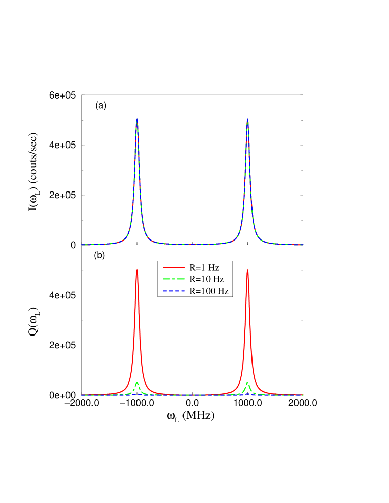
Figure 6: Case 1 ($R\ll\Gamma\ll\nu$) in the steady-state limit. Exact results for lineshape, Eq. (128), and for $Q$, Eqs. (183), (184), are shown for the strong, slow modulation case as functions of $\omega_{L}$. Parameters are chosen as $\nu=1\mbox{GHz}$, $\Gamma=100\mbox{MHz}$, $\Omega=\Gamma/10$, $R=1\mbox{Hz}-100\rm{Hz}$, and $T\to\infty$. They mimic a SM coupled to a single slow two level system in a glass. Note that lineshape does not change with $R$ while $Q$ does.

VI.1.1 strong modulation : case 1

When the $\Gamma\ll\nu$, case 1, the two intensities $I_{\pm}$ are well separated by the amplitude of the frequency modulation, $2\nu$, therefore we can approximate $\langle I\rangle\simeq I_{+}/2$ when $I_{-}\simeq 0$ and vice versa, which leads to

$$\langle(\Delta I)^{2}\rangle\simeq\langle I\rangle^{2}.\mbox{\makebox[72.26999pt][r]{$\Gamma\ll\nu$}}$$ (72)

In this case $Q$ is given by

$$Q\simeq\left\{\begin{array}[]{cc}{\langle I\rangle R^{-1}}&\mbox{\makebox[72.26999pt]{$T\gg 1/R$}}\vspace{.2cm}\\ {\langle I\rangle T}&\mbox{\makebox[72.26999pt]{$T\ll 1/R$}}.\end{array}\right.$$ (75)

We show the lineshapes and $Q$ as functions of the laser frequency $\omega_{L}$ at the steady-state limit ($T\to\infty$) for case 1 in Fig. 6. In all the calculations shown in figures of the present work, we have assumed an ideal measurement, $\eta=1$. Values of parameters are given in the figure caption. This is relevant for the case that a chromophore is strongly coupled to a single two level system in a low temperature glasszumbusch-prl-93 ; fleury-jlum-93 . Since $Q\simeq\langle I\rangle/R$ in this case, both the lineshape (Fig. 6(a)) and $Q$ (Fig. 6(b)) are similar to each other; two Lorentzian peaks located at $\omega_{L}=\pm\nu$ with widths $\Gamma$. Note that in this limit the value of $Q$ is very large compared with that in the fast modulation regime considered later. While the lineshape is independent of $R$ in this limit, the magnitude of $Q$ decreases with $R$, hence it is $Q$ not $\langle I\rangle$ which yields information on the dynamics of the environment.

VI.1.2 weak modulation : case 2

On the other hand, in case 2, where the fluctuation is very weak ($\nu\ll\Gamma$), we notice that $I_{+}\simeq I_{-}$ from Eq. (62) (note that when there is no spectral diffusion, $\nu=0$, $I_{+}=I_{-}$, thus $Q=0$). The lineshape is given by a single Lorentzian centered at $\omega_{L}=0$,

$$\langle I\rangle\simeq{\Omega^{2}\Gamma/4\over\omega_{L}^{2}+\Gamma^{2}/4}.$$ (76)

Since $\nu\ll\Gamma$ in this case we expand $I_{\pm}$ in terms of $\nu$ to find

$$\langle(\Delta I)^{2}\rangle\simeq{\nu^{2}}\left({d\langle I\rangle\over d\omega_{L}}\right)^{2}={\nu^{2}\Omega^{4}\Gamma^{2}\omega_{L}^{2}\over 4(\omega_{L}^{2}+\Gamma^{2}/4)^{4}}.\mbox{\makebox[72.26999pt]{$\nu\ll\Gamma$}}$$ (77)

Therefore, in case 2, $Q$ is given by

$$Q\simeq\left\{\begin{array}[]{cc}{{\nu^{2}\over\langle I\rangle}{\left(d\langle I\rangle\over d\omega_{L}\right)}^{2}{R^{-1}}}&\mbox{\makebox[72.26999pt]{$T\gg 1/R$}}\vspace{.2cm}\\ {{\nu^{2}\over\langle I\rangle}{\left(d\langle I\rangle\over d\omega_{L}\right)}^{2}T}&\mbox{\makebox[72.26999pt]{$T\ll 1/R$}}.\end{array}\right.$$ (80)

Note that $Q\propto{1\over\langle I\rangle}({d\langle I\rangle\over d\omega_{L}})^{2}$ in the weak, slow modulation case while $Q\propto\langle I\rangle$ in the strong, slow modulation case.

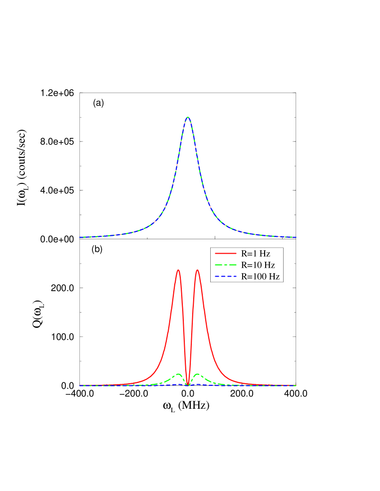
Figure 7: Case 2 ($R\ll\nu\ll\Gamma$) in the steady-state limit. Exact results for lineshape, Eq. (128), and for $Q$, Eqs. (183), (184), are shown for the weak, slow modulation case as functions of $\omega_{L}$. Parameters are chosen as $\nu=1\mbox{MHz}$, $\Gamma=100\mbox{MHz}$, $\Omega=\Gamma/10$, $R=1\rm{Hz}-100\rm{Hz}$, and $T\to\infty$.

In Fig. 7 we show the lineshape and $Q$ for the weak, slow modulation limit, case 2. The lineshape (Fig. 7 (a)) is a Lorentzian with a width $\Gamma$, to a good approximation, thus the features of the lineshape do not depend on the properties of the coupling of the SM to a environment such as $\nu$ and $R$. On the other hand, $Q$ (Fig. 7 (b)), shows a richer behavior. Recalling Eq. (80) for $T\gg 1/R$ in Eq. (77), it exhibits doublet peaks separated by $\sim{\cal{O}}(\Gamma)$ with the dip located at $\omega_{L}=0$, and its magnitude is proportional to $1/R$. We will later show that this kind of a doublet and a dip in $Q$ is a generic feature of the weak coupling case, found not only in the slow but also in the fast modulation case considered in the next section. Note that when the SM is not coupled to the environment ($\nu=0$), $Q=0$ as expected.

Both in the strong (Fig. 6) and the weak (Fig. 7) cases, we find $Q(\omega_{L}=0)\simeq 0$. This is expected in the slow modulation case considered here. Physically, when the laser detuning frequency is exactly in the middle of two frequency shifts, $\pm\nu$, the rate of photon emissions is identical whether the molecule is in the up state ($+\nu$) or in the down state ($-\nu$). Therefore, the effect of bath fluctuation on the photon counting statistics is negligible, which leads to Poissonian counting statistics at $\omega_{L}=0$.

VI.1.3 time–dependence

Additional information on the environmental fluctuations can be gained by measuring the time dependence of $Q$ in the slow modulation regime. In Fig. 8 we show $Q$ versus the measurement time $T$ for the strong, slow modulation limit, case 1, both for the exact result calculated in Appendix A and for the approximate result, Eq. (67). We choose the resonance condition $\omega_{L}=\nu$, and used parameters relevant to SMS in glass systems. The approximate result based on the two state random walk model, Eq. (67), shows a perfect agreement with the exact result in Fig. 8(a) as expected. When $T\ll 1/R$, $Q$ increases linearly with $T$ as predicted from Eq. (71) for $RT\ll 1$, and it reaches the steady-state value given by Eq. (71) when $T$ becomes $RT\gg 1$. We also notice that even in the long measurement time limit the value of $Q$ is large: $Q=5\times 10^{5}\eta$ in the example given in Fig. 8(a) (including the detection efficiency). Therefore, even if we consider the imperfect detection of the photon counting device (for example, $\eta=15\rm{\%}$ has been reported recentlyambrose-cpl-97 ), deviation of the photon statistics from Poissonian is observable in the slow modulation regime of SMS. This is seemingly contrary to propositions made in the literature mandel-optical-95 ; chen-bpj-99 ; schenzle-pra-86 , in which the claim is made that the Poissonian distribution is achieved in the long time limit. We defer discussion of this issue to the end of this section. We note that it has been shown that $Q(T)$ can be very large ($Q\sim 10^{4}$) at long times in the atomic three-level system with a metastable state but without a spectral diffusion processkim-pra-87 . Fig. 8(b) illustrates that the steady-state value of $Q(T)$ is reached when $RT\gg 1$, and the magnitude of $Q$ in the steady-state decreases as $1/R$ as predicted from Eq. (71) for $RT\gg 1$. This therefore illustrates that valuable information on the bath fluctuation timescales can be obtained by measuring the fluctuation of the lineshape as a function of measurement time.

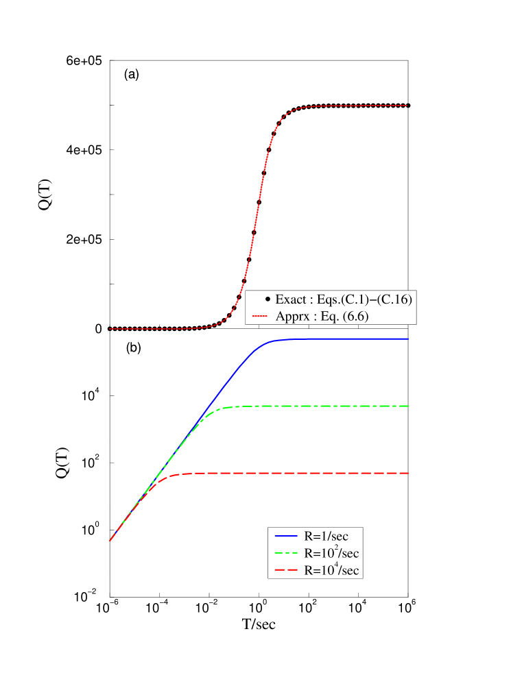
Figure 8: Case 1 ($R\ll\Gamma\ll\nu$) in the time–dependent regime. (a) $Q(T)$ is shown both for the exact result and for the approximate result given in the linear-log scale. This figure demonstrates that our exact results given in Appendix A are well reproduced by the approximation, Eq. (67). The same parameters are used as in Fig. 6 except $\omega_{L}=\nu=1\mbox{GHz}$, $R=1\mbox{Hz}$, and $T$ (varied). (b) $Q(T)$ for different values of $R$ in the slow modulation regime in the log-log scale. All the parameters except for $R$ are chosen the same as those in (a).

Fig. 9 shows a two–dimensional plot of $Q$ as a function of the laser frequency and the measurement time for the parameters chosen in Fig. 8(a). We observe that two Lorentzian peaks located at resonance frequencies become noticeable when $T\simeq 1/R$. Similar time dependent behavior can be also found for the weak, slow modulation limit, case 2, however, then $Q$ along the $\omega_{L}$ axis shows doublet peaks separated by $\sim{\cal{O}}(\Gamma)$ as shown in Fig. 7.

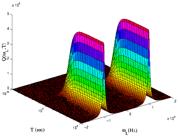
Figure 9: Case 1 ($R\ll\Gamma\ll\nu$) in the time dependent case. Two dimensional plot of $Q(\omega_{L},T)$ for the slow modulation as a function of $\omega_{L}$ and $T$. The same parameters are used as in Fig. 8(a) except $\omega_{L}$ (varied).

We can extend our result and describe photon statistics beyond the second moment. Based on the central limit theorem, the probability density function of the two state random walk variable $W$ in the long time limit is described by

$$P(W,T)\stackrel{{\scriptstyle RT\gg 1}}{{\longrightarrow}}G(W,T)\equiv{1\over\sqrt{4\pi DT}}\exp\left[-{\left(W-VT\right)^{2}\over 4DT}\right]$$ (81)

with $D=\langle(\Delta I)^{2}\rangle/(2R)$ and $V=\langle I\rangle$ when $\eta=1$. We also note that $Q\simeq 2D/V$ in the long time limit. By using Eq. (29)

$$\langle p(n,T)\rangle\simeq\int_{0}^{\infty}{\rm d}WG(W,T){W^{n}\over n!}\exp(-W).$$ (82)

Eq. (82) shows that in the long time limit the photon statistics is the Poisson transformsaleh-photoelec-78 of a Gaussian. This transformation can be found explicitly (one can slightly improve this approximation by considering a normalized truncated Gaussian with $G(W,T)=0$ for $W<0$; we expect that our approximation will work well when $V^{2}T\gg D$). In contrast to Eq. (81), the proposed Eq. (30) suggests that $G(W,T)$ be replaced with a delta function, for which a single parameter $V$ controls the photon statistics, while according to our approach both $V$ and $D$, or equivalently, $\langle W\rangle$ and $Q$ are important. Mathematically, when $T\to\infty$ the Gaussian distribution, Eq. (81) may be said to “converge” to the delta function distribution, Eq. (30), in a sense that the mean is $\langle W\rangle\sim{\cal{O}}(T)$ while the standard deviation is $\Delta W=(\langle W^{2}\rangle-\langle W\rangle^{2})^{1/2}\sim{\cal{O}}(T^{1/2})$. This argument corresponds to the proposition made in the literature, Eq. (30), and then the photon statistics is only determined by the mean $\langle W\rangle\simeq VT$. However, physically it is more informative and meaningful to consider not only the mean $\langle W\rangle$ but also the variance $(\Delta W)^{2}\simeq 2DT\simeq Q\langle W\rangle$ since it contains information on the bath fluctuation. In a sense the delta function approximation might be misleading since it implies that $Q=0$ in the long time limit, which is clearly not true in general.

VI.2 Fast Modulation Regime : $\nu,\Gamma\ll R$

In this section we consider the fast modulation regime, $\nu,\Gamma\ll R$. Usually in this fast modulation regime, the dynamics of the bath (here modeled with $R$) is so fast that only the long time limit of our solution should be considered [i.e. Eqs. (183) and (184)]. Hence all our results below are derived in the limit of $T\to\infty$, since the time dependence of $Q$ is irrelevant. The fast modulation regime considered in this section includes case 3 ($\Gamma\ll\nu\ll R$) as the strong, fast modulation case and case 4 ($\nu\ll\Gamma\ll R$) as the weak, fast modulation case.

It is well known that the lineshape is Lorentzianmukamel-nonlinear-95 in the fast modulation regime (soon to be defined precisely),

$$\langle I\left(\omega_{L}\right)\rangle={{\Omega}^{2}(\Gamma+\Gamma_{f})\over 4\omega_{L}^{2}+{(\Gamma+\Gamma_{f})^{2}}},$$ (83)

where $\Gamma_{f}$ is the line width due to the dephasing induced by the bath fluctuations and given by

$$\Gamma_{f}={\nu^{2}\over R}.$$ (84)

The lineshape given in Eq. (83) exhibits motional narrowing, namely as $R$ is increased the line becomes narrower and in the limit $R\to\infty$ the width of the line is simply $\Gamma$.

Now we define the fast modulation regime considered in this work. When $R\to\infty$ (and other parameters fixed) $Q\to 0$, so fluctuations become Poissonian. This is expected and in a sense trivial because the molecule cannot respond to the very fast bath, so the two limits $R\to\infty$ and $\nu=0$ (i.e., no interaction with the bath) are equivalent. It is physically more interesting to consider the case that $R\to\infty$ with $\Gamma_{f}/\Gamma$ remaining finite, which is the standard definition of the fast modulation regimekubo-fluct-62 . In this fast modulation regime the well known lineshape is Lorentzian as given in Eq. (83) with a width $\Gamma+\Gamma_{f}$.

Here we present a simple calculation of $Q$ in the fast modulation regime based on physically motivated approximations. We justify our approximations by comparing the resulting expression with our exact result, Eqs. (183) and (184). When the dynamics of the bath is very fast, the correlation between the state of the molecule during one pulse interval with that of the following pulse interval is not significant in the stochastic averaging Eq. (49). Therefore in the fast modulation regime, we can approximately factorize the three–time correlation function $C_{3}^{m}(\tau_{1},\tau_{2},\tau_{3})$ in Eq. (49) in terms of one–time correlation functions $C_{1}^{l}(\tau)$ as was done by Mukamel and Loring in the context of four wave mixing spectroscopymukamel-josab-86 ,

$$C_{3}^{m}(\tau_{1},\tau_{2},\tau_{3})$$ (85)

$$= \left\langle e^{-ia\int_{t_{I}}^{t_{II}}\Delta\omega(t^{\prime}){\rm d}t^{\prime}-ib\int_{t_{II}}^{t_{III}}\Delta\omega(t^{\prime}){\rm d}t^{\prime}-ic\int_{t_{III}}^{t_{IV}}\Delta\omega(t^{\prime}){\rm d}t^{\prime}}\right\rangle$$

$$\simeq \left\langle e^{-ia\int_{t_{I}}^{t_{II}}\Delta\omega(t^{\prime}){\rm d}t^{\prime}}\right\rangle\left\langle e^{-ib\int_{t_{II}}^{t_{III}}\Delta\omega(t^{\prime}){\rm d}t^{\prime}}\right\rangle\left\langle e^{-ic\int_{t_{III}}^{t_{IV}}\Delta\omega(t^{\prime}){\rm d}t^{\prime}}\right\rangle$$

$$= C_{1}^{a}(\tau_{1})C_{1}^{b}(\tau_{2})C_{1}^{c}(\tau_{3}),$$

where $a$, $b$, and $c$ are values of $S_{m}(t)$ in time intervals, $t_{I}<t<t_{II}$, $t_{II}<t<t_{III}$, and $t_{III}<t<t_{IV}$, respectively. For example, $a=-1$, $b=0$, and $c=1$ for the case $m=1$ (see Table 1). The one–time correlation function is evaluated using the second order cumulant approximation, which is also valid for the fast modulation regimemukamel-josab-86 ,

$$C_{1}^{l}(t)\simeq\exp\left(-l^{2}\int_{0}^{t}{\rm d}t^{\prime}\int_{0}^{t^{\prime}}{\rm d}t^{\prime\prime}\langle\Delta\omega(t^{\prime})\Delta\omega(t^{\prime\prime})\rangle\right).$$ (86)

Note that these two approximations, Eqs. (85) and (86), are not limited to the two state jump model but are generally valid in the fast modulation regime. The frequency correlation function is given by

$$\langle\Delta\omega(t^{\prime})\Delta\omega(t^{\prime\prime})\rangle=\nu^{2}\exp(-2R|t^{\prime}-t^{\prime\prime}|)$$ (87)

for the two state jump model. Substituting Eq. (87) into Eq. (86) we have

$$C_{1}^{l}(t)\simeq\exp\left[-l^{2}\nu^{2}\left({t\over 2R}+{e^{-2Rt}-1\over(2R)^{2}}\right)\right].$$ (88)

In the limit of $R\to\infty$ we can approximate $C_{1}^{l}(t)$ further

$$C_{1}^{l}(t)\simeq\exp(-l^{2}\Gamma_{f}t/2),$$ (89)

and in turn evaluate all the three–time correlation functions corresponding to different time orderings within these approximations using Eqs. (85) and (89). We note that the lineshape shows a Lorentzian behavior with the width $\Gamma+\Gamma_{f}$ in Eq. (83) because of the exponential decay of the one–time correlation function in Eq. (89). Since we have simple analytical expressions of the three–time correlation functions, it is straightforward to calculate $Q$ in the fast modulation regime. After straightforward algebra described in Appendix D, $Q$ in the fast modulation regime is

$$Q={{\Omega^{2}\Gamma_{f}}\left[8\Gamma_{f}\omega_{L}^{4}+2(\Gamma+\Gamma_{f})(8\Gamma^{2}+15\Gamma\Gamma_{f}+5\Gamma_{f}^{2})\omega_{L}^{2}+\Gamma_{f}(\Gamma+2\Gamma_{f})(\Gamma+\Gamma_{f})^{3}\right]\over{16\Gamma(\Gamma+\Gamma_{f})\left(\omega_{L}^{2}+{(\Gamma+\Gamma_{f})^{2}\over 4}\right)^{2}\left(\omega_{L}^{2}+{(\Gamma+2\Gamma_{f})^{2}\over 4}\right)}}.$$

(90)

Note that the exact expression for $Q$ obtained in Appendix B yields the same expression as Eq. (90) when $R\to\infty$ but $\Gamma_{f}$ remains finite, which justifies the approximations introduced.

Let us now estimate the magnitude of these fluctuation. We consider $\omega_{L}=0$ since the photon current is strongest for this case (i.e., the lineshape has a maximum at $\omega_{L}=0$), then

$$Q=\frac{4\,\eta\,\Omega^{2}\,\Gamma_{f}^{2}}{\Gamma\,{\left(\Gamma+\Gamma_{f}\right)}^{2}\,\left(\Gamma+2\,\Gamma_{f}\right)},$$ (91)

where the detection efficiency $\eta$ has been restored. The maximum of $Q$ is found when $\Gamma_{f}=\Gamma(1+\sqrt{5})/2$ and then $Q\simeq 0.361\eta\Omega^{2}/\Gamma^{2}$. Even if we take $|\Omega|/\Gamma=1/10$ and $\eta=5\times 10^{-2}$ as reasonable estimates for a weak laser field and detection efficiency we find $Q\simeq 2\times 10^{-4}\ll 1$ which shows the difficulties of measuring deviations from Poissonian statistics in this limit. We note, however, that values of $Q$ as small as $|Q|\leq 10^{-4}$ have been measured recently (although in the short time regime, not in the steady-state case)fleury-prl-00 . Therefore it might also be possible to observe the deviation from Poissonian photon statistics in the fast modulation limit under appropriate experimental situations.

In Fig. 10 we show the results of exact steady-state calculations for the lineshape and $Q$ [Eq. (183) and (184)] for different values of the fluctuation rate $R$ in the fast modulation regime. We have chosen the parameters as $\nu=100\rm{MHz}$, $\Gamma=1\rm{MHz}$, and $\Omega=\Gamma/10$, and $R$ is varied from $1\rm{GHz}$ to $100\rm{GHz}$, corresponding to case 3. For this parameter set we have checked that the fast modulation approximation for $Q$ given in Eq. (90) agrees well with the exact calculation, Eqs. (183), (184).

The lineshape shown in Fig. 10(a) shows the well known motional narrowing behavior. When $R=1\rm{GHz}$, the lineshape is a broad Lorentzian with the width $\Gamma+\Gamma_{f}\simeq\Gamma_{f}$ (note that $\Gamma_{f}\gg\Gamma$ in this case). As $R$ is increased further the line becomes narrowed and finally its width is given by $\Gamma$ as $R\to\infty$.

Compared with the lineshape, $Q$ in Fig. 10(b) shows richer behavior. The most obvious feature is that when $R\to\infty$, $Q\to 0$. This is expected since when the bath is very fast the molecule cannot respond to it, hence fluctuations are Poissonian and $Q\to 0$. It is noticeable that, unlike $I(\omega_{L})$, $Q$ shows a type of narrowing behavior with splitting as $R$ is increased. The lineshape remains Lorentzian regardless of $\Gamma_{f}$ in the fast modulation case, while $Q$ changes from a broad Lorentzian line with the width $\Gamma_{f}$ when $\Gamma_{f}\gg\Gamma$ to doublet peaks separated approximately by $\Gamma$ when $\Gamma_{f}\ll\Gamma$, that will be analyzed in the following [see, for example, Eq. (94)]. Therefore, although the value of $Q$ is small in the fast modulation regime, it yields additional information on the relative contributions of $\Gamma$ and $\Gamma_{f}$ which are not differentiated in the lineshape measurement.

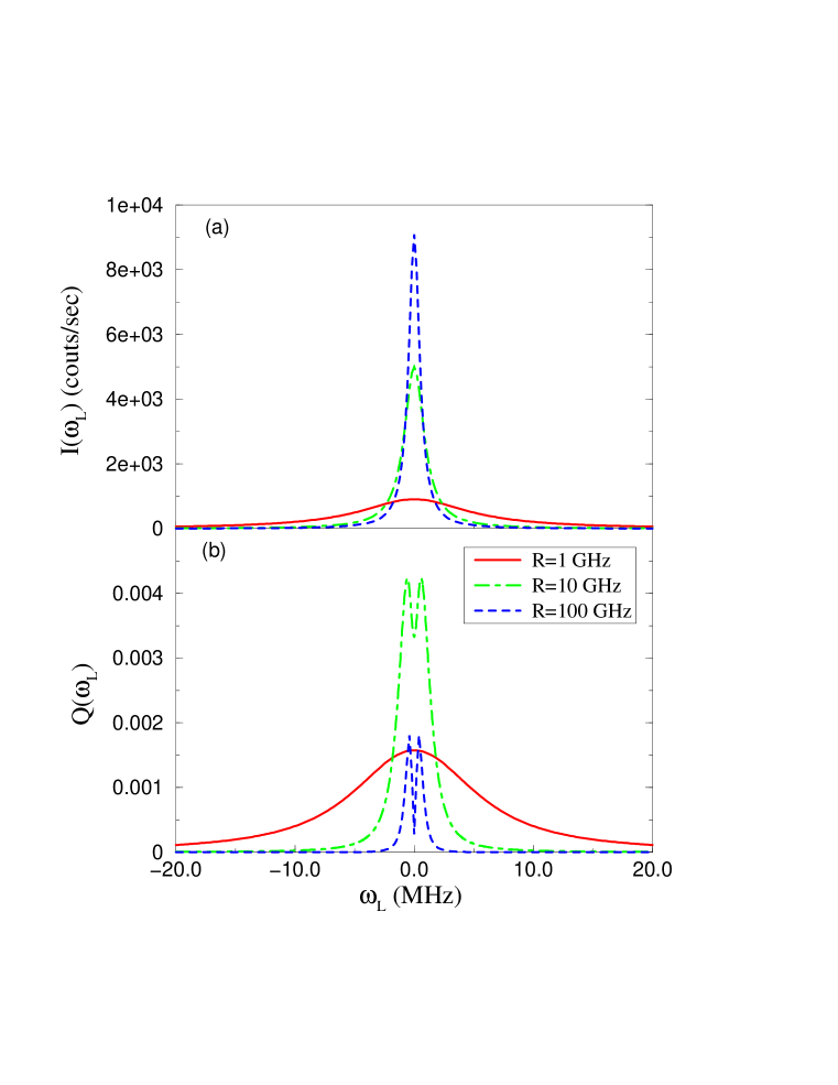
Figure 10: Case 3 ($\Gamma\ll\nu\ll R$) in the steady-state limit. Lineshape and $Q$ in the fast modulation regime are shown as functions of $\omega_{L}$. Parameters are chosen as $\nu=100\rm{MHz}$, $\Gamma=1\rm{MHz}$, $\Omega=\Gamma/10$, $R=1\rm{GHz}-100\rm{GHz}$, and $T\to\infty$.

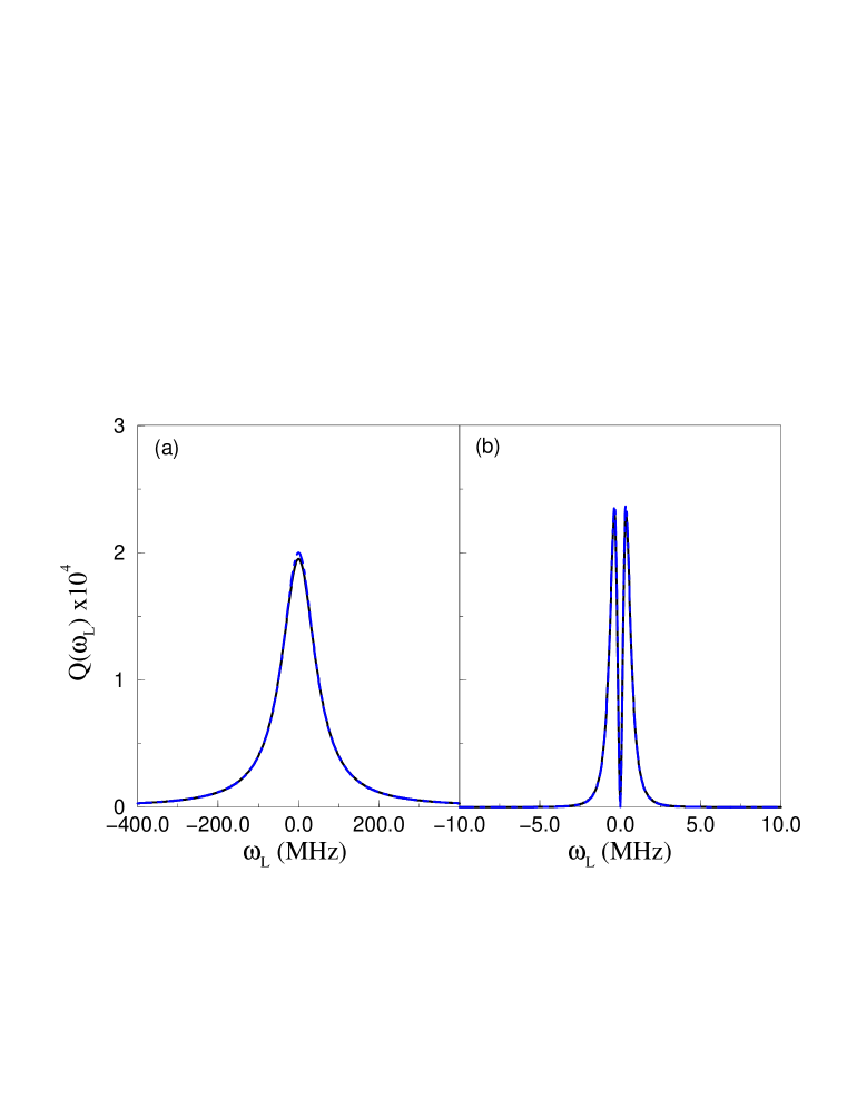
Figure 11: Case 3 ($\Gamma\ll\nu\ll R$) in the steady-state limit. Exact calculations (solid line) of $Q$, Eqs. (183) and (184) are compared with the approximate expressions, Eq. (94), (dashed line) for (a) the Lorentzian ($\Gamma_{f}\gg\Gamma$), and (b) the splitting ($\Gamma_{f}\ll\Gamma$) cases in the fast modulation case. Parameters are chosen as $\nu=1\rm{GHz}$, $\Gamma=1\rm{MHz}$, $\Omega=\Gamma/10$, $T\to\infty$, and $R=10\rm{GHz}$ in (a) while $R=10^{5}\rm{GHz}$ in (b).

VI.2.1 strong modulation : case 3

We further analyze the case that the bath fluctuation is both strong and fast, case 3, $\Gamma\ll\nu\ll R$. The results shown in Fig. 10 correspond to this case. We find that Eq. (90) is further simplified in two different limits, $\Gamma_{f}\gg\Gamma$ and $\Gamma_{f}\ll\Gamma$,

$$Q\simeq\left\{\begin{array}[]{cc}\frac{{\Omega}^{2}\,\Gamma_{f}}{2\Gamma\left(\omega_{L}^{2}+\Gamma_{f}^{2}/4\right)}&\mbox{\makebox[72.26999pt]{$\Gamma_{f}\gg\Gamma$}}\vspace{.2cm}\\ \frac{{\Omega}^{2}\,\Gamma_{f}\,\Gamma\,\omega_{L}^{2}}{\,\left(\omega_{L}^{2}+\Gamma^{2}/4\right)^{3}}&\mbox{\makebox[72.26999pt]{$\Gamma_{f}\ll\Gamma$}}\end{array}\right.$$ (94)

When $\Gamma_{f}\gg\Gamma$, both $Q$ and the lineshape are a Lorentzian located at $\omega_{L}=0$ with a width $\Gamma_{f}$, which yields the relation $Q\simeq 2\langle I(\omega_{L})\rangle/\Gamma$, and both exhibit motional narrowing behaviors. In the other limit, $\Gamma_{f}\ll\Gamma$, we have neglected ${\cal{O}}((\Gamma_{f}/\Gamma)^{2})$ terms with additional conditions for $\omega_{L}^{2}$, ${\Gamma_{f}\over\Gamma}\ll{\left({\omega_{L}\over\Gamma}\right)}^{2}\ll{\Gamma\over\Gamma_{f}}$. In this case $Q$ shows a splitting behavior at $|\omega_{L}|\sim{\cal{O}}(\Gamma)$. We note that Eq. (94) for $\Gamma_{f}\ll\Gamma$ is the same as Eq. (80) This is the case because the very fast frequency modulation corresponds to the weak modulation case, if we recall that the dephasing rate due to the bath fluctuation is given by $\Gamma_{f}=\nu^{2}/R$ in the fast modulation regime.

In Fig. 11 we have checked the validity of the limiting expressions of $Q$ for the Lorentzian and the splitting cases (Eq. (94) by comparing to the exact results, Eqs. (183), (184). In Fig. 11(a), the parameters are chosen such that $\Gamma_{f}=100\Gamma$ while in Fig. 11(b) $\Gamma_{f}=\Gamma/100$. Approximate expressions (dashed line) show a good agreement with exact expressions (solid line) in each case.

VI.2.2 weak modulation : case 4

Now we consider the weak, fast modulation case, case 4 ($\nu\ll\Gamma\ll R$). In this limit, the lineshape is simply a single Lorentzian peak given by Eq. (83) with $\Gamma+\Gamma_{f}\simeq\Gamma$. We obtain the following limiting expression for $Q$ from Eq. (90), noting $\Gamma_{f}=\nu^{2}/R$,

$$Q\simeq\frac{\nu^{2}\,{\Omega}^{2}\,\Gamma\,\omega_{L}^{2}}{R\left(\omega_{L}^{2}+\Gamma^{2}/4\right)^{3}}.$$ (95)

Also here $Q$ shows splitting behavior. It is given by the same expression as that in the strong, fast modulation case with $\Gamma_{f}\ll\Gamma$ (see Eq. (94)) and also as that in the weak, slow modulation case with $T\gg 1/R$ (see Eq. (80)) (see also Table 2 in Section VI.4). When $Q$ is plotted as a function of $\omega_{L}$, it would look similar to Fig. 11(b).

VI.3 Intermediate Modulation Regime

So far we have considered four limiting cases: (i) strong, slow, (ii) weak, slow, (iii) strong, fast, and (iv) weak, fast case. We now consider case 5 ($\Gamma\ll R\ll\nu$) and case 6 ($\nu\ll R\ll\Gamma$). They are neither in the slow nor in the fast modulation regime according to our definition.

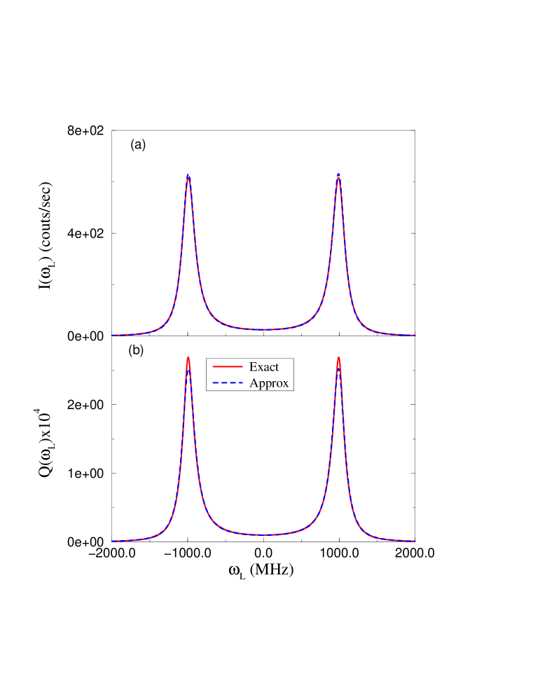
Figure 12: Case 5 ($\Gamma\ll R\ll\nu$) in the steady-state limit. Exact results for lineshape, Eq. (128), and for $Q$, Eqs. (183), (184), are compared with approximations corresponding to $\Gamma\rightarrow 0$ limit, Eqs. (133) and (185), respectively. Parameters are chosen as $\nu=1\mbox{GHz}$, $\Gamma=5\mbox{MHz}$, $\Omega=\Gamma/10$, $R=100\mbox{MHz}$, and $T\to\infty$.

VI.3.1 case 5

In case 5($\Gamma\ll R\ll\nu$), the bath fluctuation is fast compared with the radiative decay rate but not compared with the fluctuation amplitude. Because $\Gamma\ll R,\nu$ in this case we can approximate the exact results for $\langle I\rangle$ and $Q$ by their limiting expressions corresponding to $\Gamma\rightarrow 0$, yielding Eqs. (133) and (185), and an important relation holds in this limit,

$$\lim_{\Gamma\rightarrow 0}Q={2\over\Gamma}\lim_{\Gamma\rightarrow 0}\langle I\rangle.$$ (96)

Note that the same relation between $Q$ and $\langle I\rangle$ was also found to be valid in one of the fast modulation regimes, Eq. (94) with $\Gamma_{f}\gg\Gamma$. Fig. 12 shows that in this case the limiting expressions approximate well the exact results.

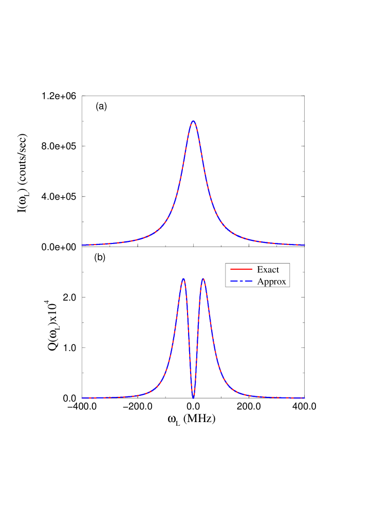
Figure 13: Case 6 ($\nu\ll R\ll\Gamma$) in the steady-state limit. Exact results for lineshape, Eq. (128), and for $Q$, Eqs. (183), (184), are compared with approximations corresponding to $\nu\rightarrow 0$ limit, Eqs. (76) and (97), respectively, Parameters are chosen as $\nu=1\mbox{MHz}$, $\Gamma=100\mbox{MHz}$, $\Omega=\Gamma/10$, $R=10\mbox{MHz}$, and $T\to\infty$.

VI.3.2 case 6

In case 6, since $\nu\ll R\ll\Gamma$ we can approximate the exact results by considering small $\nu$ limit in Eqs. (183) and (184) for $Q$, and Eq. (128) for the lineshape. By taking this limit, we find that the lineshape is well described by a single Lorentzian given by Eq. (76), and $Q$ by Eq. (80). We note that for all weak modulation cases, cases 2, 4, and 6, the lineshape and $Q$ behave in a unique way described by Eq. (76) and Eq. (80) for $RT\gg 1$, respectively, and both the slow and fast modulation approximate results are valid in this case (see Table 2). Also a simple relation between $\langle I\rangle$ and $Q$ holds in the limit, $\nu\to 0$,

$$\lim_{\nu\to 0}Q={\nu^{2}\over R}\lim_{\nu\to 0}{1\over\langle I\rangle}\left(d\langle I\rangle\over d\omega_{L}\right)^{2}.$$ (97)

The exact results of lineshape and $Q$ in Fig. 13 show good agreement with the approximate results, Eqs. (76) and (97).

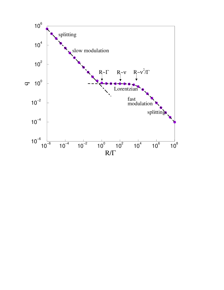
Figure 14: $q$ versus $R/\Gamma$ in the strong modulation case. Filled circles are the result of exact calculation based on Eqs. (183) and (184) when $\nu/\Gamma=100$. The dot-dashed and dashed curves are calculations based on approximate expressions of $Q$, Eq. (75) (slow modulation case) and Eq. (90) (fast modulation case), respectively.

VI.4 Phase Diagram

We investigate the overall effect of the bath fluctuation on the photon statistics for the steady-state case as the fluctuation rate $R$ is varied from slow to fast modulation regime. To characterize the overall fluctuation behavior of the photon statistics, we define an order parameter $q$,

$$q\equiv{\Gamma\over\pi\Omega^{2}}\int_{-\infty}^{\infty}Q(\omega_{L}){\rm{d}}\omega_{L},$$ (98)

where $Q$ in the steady state is given in Eqs. (183) and (184). Before we discuss the behavior of $q$ it is worthwhile mentioning that the lineshape is normalized to a constant regardless of $R$ and $\Gamma$,

$$\int_{-\infty}^{\infty}\langle I(\omega_{L})\rangle{\rm{d}}\omega_{L}={\pi\Omega^{2}\over 2},$$ (99)

which can be easily verified from Eq. (45). In contrast, $q$ exhibits nontrivial behavior reminiscent of a phase transition. In Figs. 14 and 15 we show $q$ versus $R/\Gamma$. The figures clearly demonstrate how the photon statistics of SMS in the presence of the spectral diffusion becomes Poissonian as $R\to\infty$ or $\nu\to 0$ (i.e. $q\to 0$ when $R\to\infty$ or $\nu\to 0$).

We first discuss the strong modulation regime, $\nu\gg\Gamma$, shown in Fig. 14 with $\nu/\Gamma=100$ in this case. Depending on the fluctuation rate, there are three distinct regimes:

(a) In the slow modulation regime, $R\ll\Gamma$, $q$ decreases as $1/R$. The approximate calculation (dot-dashed line) based on the slow modulation approximation, Eq. (75) shows good agreement with the exact calculation.

(b) When $R$ is such that $\Gamma\ll R\ll\nu$ [case 5], the intermediate regime is achieved, and $q$ starts to show a plateau behavior. The plateau behavior is found whenever $Q=2\langle I(\omega_{L})\rangle/\Gamma$, which yields $q=1$ as can be easily seen from Eqs. (98) and (99). As $R$ is increased further such that $\nu\ll R$, the fast modulation regime is reached, and $q$ still shows a plateau until $R\simeq\nu^{2}/\Gamma$. In this regime the Lorentzian behavior of $Q$ is observed in Eq. (94) for $\Gamma_{f}\gg\Gamma$.

(c) When the bath fluctuation becomes extremely fast such that $R\gg\nu^{2}/\Gamma$, the splitting behavior of $Q$ is observed, as discussed in Eq. (94) for $\Gamma_{f}\ll\Gamma$, and then $q\propto 1/R$ similar to the slow modulation regime. The approximate value of $q$ based on fast modulation approximation, Eq. (90) (dotted line) shows good agreement with the exact calculation found using Eqs. (183) and (184). Finally, when $R\to\infty$, $Q=0$. As mentioned this is expected since the molecule cannot interact with a very fast bath hence the photon statistics becomes Poissonian.

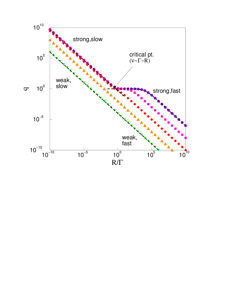
Figure 15: Phase diagram of $q$ versus $R/\Gamma$. Symbols are the results of exact calculations based on Eqs. (183) and (184) as $\nu/\Gamma$ is varied from the lower-left to the upper-right cases: $0.01$ (downward triangle), $0.1$ (upward triangle), $1$ (diamond), $10$ (square), $100$ (circle). The dashed curves are calculations based on appropriate approximate expressions of $Q$ for each case, Eqs. (95) (weak modulation), (75) (strong, slow modulation), and (90) (strong, fast modulation).

Now we discuss the effect of magnitude of frequency fluctuation, $\nu$, on $q$ in Fig. 15. We have calculated $q$ as a function of $1/R$ as $\nu$ is varied from $\nu/\Gamma=100$ (circles) to $\nu/\Gamma=0.01$ (downward triangles). We see in Fig. 15 that the $(q,R/\Gamma)$ diagram exhibits a behavior similar to a phase transition as $\nu$ is varied. In the strong modulation regime ($\nu/\Gamma\gg 1$), three distinct regimes appear in the $(q,R/\Gamma)$ diagram ($R\leq\Gamma$, $\Gamma\leq R\leq\nu^{2}/\Gamma$, and $R\geq\nu^{2}/\Gamma$), while in the weak modulation regime ($\nu/\Gamma\ll 1$) $q$ always decreases as $1/R$. When three parameters, $\nu$, $\Gamma$, and $R$, have similar values, $\nu\sim\Gamma\sim R$, there appears a “critical point” in the “phase diagram”.

Table 2 summarizes various expressions for the lineshape and $Q$ found in the limiting cases of the two state jump model investigated in this work. For simplicity, we have set $\eta=1$. We see that although the fluctuation model itself is a simple one, rich behaviors are found. We believe that these behaviors are generic (although we do not have a mathematical proof). In the weak modulation cases, both $\langle I\rangle$ and $Q$ can be described by a single expression, irrespective of the fluctuation rate $R$. However, in the strong modulation cases, $\langle I\rangle$ and $Q$ change their qualitative features as $R$ changes.

	slow	intermediate	fast
	$R\ll\nu\ll\Gamma$ : case 2	$\nu\ll R\ll\Gamma$ : case 6	$\nu\ll\Gamma\ll R$ : case 4
weak	$\displaystyle\langle I\rangle\sim{\Omega^{2}\Gamma\over 4\left[\omega_{L}^{2}+{\Gamma^{2}\over 4}\right]}$
	$\displaystyle Q\sim{\Gamma_{f}\over\langle I\rangle}\left({\rm d}\langle I\rangle\over{\rm d}\omega_{L}\right)^{2}$
	$R\ll\Gamma\ll\nu$ : case 1	$\Gamma\ll R\ll\nu$ : case 5	$\Gamma\ll\nu\ll R$ : case 3
strong	$\displaystyle\langle I\rangle\sim{I_{+}+I_{-}\over 2}$	$\displaystyle\langle I\rangle$ $\displaystyle\sim{\Omega^{2}\nu^{2}R\over(\omega_{L}^{2}-\nu^{2})^{2}+4R^{2}\omega_{L}^{2}}$	$\displaystyle\langle I\rangle\sim{\Omega^{2}(\Gamma+\Gamma_{f})\over 4\left[\omega_{L}^{2}+{(\Gamma+\Gamma_{f})^{2}\over 4}\right]}$
	$\displaystyle Q\sim{\langle I\rangle\over R}$	$\displaystyle Q\sim{2\langle I\rangle\over\Gamma}$	$\displaystyle Q$ $\displaystyle\sim\left\{\begin{tabular}[]{ll}\large${2\langle I\rangle\over\Gamma}$&$\Gamma_{f}\gg\Gamma$\vspace{.2cm}\\ \large${\Gamma_{f}\over\langle I\rangle}\left({\rm d}\langle I\rangle\over{\rm d}\omega_{L}\right)^{2}$&$\Gamma_{f}\ll\Gamma$\end{tabular}\right.$

Table 2: Parameter regimes investigated in this work are classified with expressions for the lineshape, $\langle I\rangle$, and $Q$ for each case. $I_{\pm}$ have been defined in Eq. (62).

VII Connection to Experiments

Single molecule spectroscopy has begun to reveal the microscopic nature of low temperature glassesfleury-jlum-93 ; boiron-cp-99 ; geva-jpcb-97 ; brown-jcp-98 ; barkai-prl-00 ; barkai-jcp-00 . An important question is whether the standard tunneling model of low temperature glass developed by Anderson, Halperin, Varmaanderson-philos-71 and Phillipsphillips-jltp-72 is valid or not. As far as macroscopic measurements of acoustic, thermal, and optical properties are concerned, this model has proved to be compatible with experimental resultsesquinazi-tunn-98 . However, on a more microscopic level we do not have much experimental or theoretical proof (or disproof) that the model is valid. At the heart of the standard tunneling model is the concept of a two level system(TLS). At very low temperatures, the complicated multidimensional potential energy surface of the glass system is presumed to reduce to a multitude of non–interacting double well potentials whose two local minima correspond to reorientations of clusters of atoms or moleculesheuer-prl-93 . Hence the complicated behavior of glasses is reduced to a simple picture of many non–identical and non–interacting TLSs. For a different perspective on the nature of low temperature excitation in glasses, see Ref. lubchenko-prl-01 .

Geva and Skinnergeva-jpcb-97 have provided a theoretical interpretation of the static lineshape properties in a glass (i.e. $\langle W\rangle$). The theory relied on the standard tunneling model and the Kubo–Anderson approach as means to quantify the lineshape behavior (i.e. the time dependent fluctuations of $W$ are neglected). In Ref. barkai-prl-00 , the distribution of static lineshapes in a glass was found analytically and the relation of this problem to Lévy statistics was demonstrated.

Orrit and coworkerszumbusch-prl-93 ; fleury-jlum-93 have measured spectral trails as well as the lineshapes and the fluorescent intensity correlation function $g^{(2)}(t)$. In Ref. boiron-cp-99 spectral trails of 70 molecules were investigated and 22 exhibited behaviors that seemed incompatible with the standard tunneling model. While the number of molecules investigated is not sufficient to determine whether the standard tunneling model is valid, the experiments are approaching a direct verification of this model.

Our theory in the slow modulation limit describes SMS experiments in glasses. The TLSs in the glass flip between their up and down states with a rate $R$ determined by the coupling of TLS to phonons, the energy asymmetry, and the tunneling matrix element of the TLSanderson-philos-71 ; phillips-jltp-72 . When a TLS makes a transition from the up to the down state, or vice versa, a frequency shift $\nu\propto{1/r^{3}}$ occurs in the absorption frequency of a SM, where $r$ is the distance between the SM and the TLS. The ${1/r^{3}}$ dependence is due to an elastic dipole interaction between the SM and the TLS. In a low temperature glass, the density of TLSs is very low, hence one finds in experiment that the SM is coupled strongly to only a few TLSs. In some cases, when one TLS is in the vicinity of the SM, it is a reasonable approximation to neglect all the background TLSs. In this case, our theory describes SMS for chromophores in glasses with a single TLS strongly coupled to SM. Extension of our work to coupling of SM to many TLSs is important, and can be done in a straightforward manner provided that the TLSs are not interacting with each other.

Fleury et al.fleury-jlum-93 measured $g^{(2)}(t)$ for a single terrylene molecule coupled to single TLS in polyethylene matrix. They showed that their experimental results are well described by

$$g^{(2)}(\tau)=1+{R_{+}R_{-}(I_{+}-I_{-})^{2}\over(R_{+}I_{+}+R_{-}I_{-})^{2}}e^{-(R_{+}+R_{-})\tau},$$ (100)

where $R_{+}$ and $R_{-}$ are the upward and downward transition rates, respectively. These two rates, $R_{+}$ and $R_{-}$ are due to the asymmetry of the TLS. This result is compatible with our result for $Q$ in the slow modulation limit. When Eq. (100) is used in Eq. (3) with $R_{+}=R_{-}=R$ for the symmetric transition case considered in this work, we exactly reproduce the result of $Q(T)$ for the slow modulation given in Eq. (67). [The asymmetric rate case $R_{+}\neq R_{-}$ is also readily formulated for $Q$ in the slow modulation limit, and again leads to a result compatible with Eq. (100).] Hence, at least in this limit, our results are in an agreement with the experiment.

As far as we are aware, however, measurements of photon counting statistics for SMS in fast modulation regimes have not been made yet. The theory presented here suggests that even in the fast modulation regime, the deviation from Poisson statistics due to a spectral diffusion process might be observed under suitable experimental situations, for example, when the contributions of other mechanisms such as the quantum mechanical anti-bunching process and the blinking process due to the triplet state are known a priori. In this case, it can give more information on the distribution of the fluctuation rates, the strength of the chromophore-environment interaction, and the bath dynamics than the lineshape measurement alone.

VIII Further Discussions

All along in this work we have specified the conditions under which the present model is valid. Here we will emphasize the validity and the physical limitations of our model. We will also discuss other possible approaches to the problem at hand.

In the present work, we have used classical photon counting statistics in the weak laser field limit. In the case of strong laser intensity, quantum mechanical effects on the photon counting statistics are expected to be important. From theories developed to describe two level atoms interacting with a photon field in the absence of environmental fluctuations, it is known that, for strong field cases, deviations from classical Poissonian statistics can become significantmandel-optical-95 ; plenio-rmp-98 . One of the well known quantum mechanical effects on the counting statistics is the photon anti-bunching effectfleury-prl-00 ; lounis-nature-00 ; basche-prl-92 ; michler-nature-00 ; short-prl-83 ; schubert-prl-92 . In this case, a sub-Poissonian behavior is obtained, $-1<Q_{\rm{qm}}<0$, where the subscript “qm” stands for quantum mechanical contribution. It is clear that when the spectral diffusion process is significant (i. e. cases 1 and 2) any quantum mechanical correction to $Q$ is negligibly small. However, in the fast modulation case where we typically found a small value of $Q$, for example, $Q\sim 10^{-4}$, quantum mechanical corrections due to anti-bunching phenomenon might be important unless experiments under extremely weak fields can be performed such that $|Q_{{\rm qm}}|<Q_{{\rm sd}}$, where the subscript “sd” stands for spectral diffusion. The interplay between truly quantum mechanical effects and the fast dynamics of the bath is left for future work.

In this context it is worthwhile to recall the quantum jump approach developed in the quantum optics community. In this approach, an emission of a photon corresponds to a quantum jump from the excited state to the ground state. For a molecule with two levels, this means that right after each emission event, $\rho_{ee}=0$ (i. e. the system is in the ground state). Within the classical approach this type of wavefunction collapse never occurs. Instead, the emission event is described with the probability of emission per unit time being $\Gamma\rho_{ee}(t)$, where $\rho_{ee}(t)$ is described by stochastic Bloch equation. At least in principle, the quantum jump approach, also known as the Monte Carlo wavefunction approachdum-pra-92 ; plenio-rmp-98 ; dalibard-prl-92 ; mollmer-josab-93 ; makarov-jcp-99-1 ; makarov-jcp-01 , can be adapted to calculate the photon statistics of a SM in the presence of spectral diffusion.

Another important source of fluctuation in SMS is due to the triplet state dynamics. Indeed, one of our basic assumptions was the description of the electronic transition of the molecule in terms of a two state model. Blinking behavior is found in many SMS experimentsbernard-jcp-93 ; basche-nature-95 ; brouwer-prl-98 ; vandenbout-sci-97 ; yip-jpca-98 . Due to the existence of metastable triplet states (usually long lived) the molecule switches from the bright to the dark states (i. e. when molecule is shelved in the triplet state, no fluorescence is recorded). Kim and Knightkim-pra-87 pointed out that $Q$ can become very large in the case of the metastable three level system in the absence of spectral diffusion. This is especially the case when the lifetime of the metastable state is long. Molski et al.molski-cpl-00a ; molski-cpl-00b have considered the effect of the triplet state blinking on the photon counting statistics of SMS.

Therefore at least three sources of fluctuations can contribute to the measured value of $Q$ in SMS ; (i) $Q_{\rm{qm}}$, well investigated in quantum optics community, (ii) $Q_{\rm{triplet}}$, which can be described using the approach of Ref. kim-pra-87 , and now we have calculated the third contribution to $Q$, (iii) $Q_{\rm{sd}}$. Our approach is designed to describe a situation for which the spectral diffusion process is dominant over the others.

It is interesting to see if one can experimentally distinguish $Q_{\rm{sd}}$ and $Q_{\rm{triplet}}$ for a SM in a condensed environment. One may think of the following gedanken experiment: consider a case where the SM jumps between the bright to the dark state, and assume that we can identify the dark state when the SM is in the metastable triplet state. Further, let us assume that dark state is long lived compared to the time between emission events in the bright state. Then, at least in principle, one may filter out the effect of the dark triplet state on $Q$ especially when the timescale of the spectral diffusion process is short compared with the dark period by measuring the photon statistics during the bright period.

IX Concluding Remarks

In this paper we have developed a stochastic theory of single molecule fluorescence spectroscopy. Fluctuations described by $Q$ are evaluated in terms of a three–time correlation function $C_{3}\left(\tau_{1},\tau_{2},\tau_{3}\right)$ related to the response function in nonlinear spectroscopy. This function depends on the characteristics of the spectral diffusion process. Important time ordering properties of the three–time correlation function were investigated here in detail. Since the fluctuations (i.e., $Q$) depend on the three–time correlation function, necessarily they contain more information than the lineshape which depends on the one–time correlation function $C_{1}\left(\tau_{1}\right)$ via the Wiener–Khintchine theorem.

We have evaluated the three–time correlation function and $Q$ for a stochastic model for a bath with an arbitrary timescale. The exact results for $Q$ permit a better understanding of the non–Poissonian photon statistics of the single molecule induced by spectral diffusion. Depending on the bath timescale, different time orderings contribute to the lineshape fluctuations and in the fast modulation regime all time orderings contribute. The theory predicts that $Q$ is small in the fast modulation regime, increasing as the timescale of the bath (i.e. $1/R$) is increased. We have found nontrivial behavior of $Q$ as the bath fluctuation becomes fast. Results obtained in this work are applicable to the experiment in the slow to the intermediate modulation regime (provided that detection efficiency is high), and our results in the more challenging fast modulation regime give the theoretical limitations on the measurement accuracy needed to detect $Q>0$.

The model system considered in this work is simple enough to allow an exact solution, but still complicated enough to exhibit nontrivial behavior. Extensions of the present work is certainly possible in several important aspects. It is worthwhile to consider photon counting statistics for a more complicated chromophore-bath model, for example, the case of many TLSs coupled to the chromophore, to see to what extent the results obtained in this work would remain generic. Also the effects of a triplet bottleneck state on the photon counting statistics can be investigated as a generalization of the theory presented here. Another direction for the extension of the present theory is to formulate the theory of SMS starting from the microscopic model of the bath dynamics (e. g. the harmonic oscillator bath model). Effects of the interplay between the bath fluctuation and the quantum mechanical photon statistics on SMS is also left for future work.

The standard assumption of Markovian processes (e.g. the Poissonian Kubo–Anderson processes considered here) fails to explain the statistical properties of emission for certain single “molecular” systems such as quantum dotskuno-jcp-00 ; neuhauser-prl-00 ; shimizu-prb-01 . Instead of the usual Poissonian processes, a power-law process has been found in those systems. For such highly non–Markovian dynamics stationarity is never reached and hence our approach as well as the Wiener–Khintchine theorem does not apply. This problem has been investigated in Ref. jung-qd-02 .

X Appendix A: Calculation of Lineshape

In this appendix, we calculate the lineshape for our working example. We set $J=1$ and $\omega_{0}=0$ and as mentioned the stochastic frequency modulation follows $\Delta\omega(t)=\nu h(t)$, where $h(t)$ describes a two state telegraph process with $h(t)=+1$ (up) or $h(t)=-1$ (down). Transitions from state up to down and down to up are described by the rate $R$.

We use the marginal averaging approachshore-josab-84 ; burshtein-jetp-66 ; shore-coherent-90 to calculate the average lineshape. Briefly, the method gives a general prescription for the calculation of averages $\langle y\rangle$ ($y$ is a vector) described by stochastic equation $\dot{y}=M(t)y$, where $M(t)$ is a matrix whose elements are fluctuating according to a Poissonian process (see Refs. shore-josab-84 ; shore-coherent-90 for details). We define the marginal averages, $\langle v(t)\rangle_{x}$ , $\langle u(t)\rangle_{x}$ and $\langle w(t)\rangle_{x}$ where $x=+$ or $x=-$ denotes the state of the two state process at time $t$. For the stochastic Bloch equation, the evolution equation for the marginal averages are

$$\left(\begin{array}[]{c}\langle\dot{u}\rangle_{+}\\ \langle\dot{v}\rangle_{+}\\ \langle\dot{w}\rangle_{+}\\ \langle\dot{u}\rangle_{-}\\ \langle\dot{v}\rangle_{-}\\ \langle\dot{w}\rangle_{-}\end{array}\right) = \left(\begin{array}[]{c c c c c c}-R-{\Gamma\over 2}&\delta_{L}^{+}&0&R&0&0\\ -\delta_{L}^{+}&-R-{\Gamma\over 2}&-\Omega&0&R&0\\ 0&\Omega&-\Gamma-R&0&0&R\\ R&0&0&-R-{\Gamma\over 2}&\delta_{L}^{-}&0\\ 0&R&0&-\delta_{L}^{-}&-R-{\Gamma\over 2}&-\Omega\\ 0&0&R&0&\Omega&-R-\Gamma\end{array}\right)$$ (113)

$$\times \left(\begin{array}[]{c}\langle u\rangle_{+}\\ \langle v\rangle_{+}\\ \langle w\rangle_{+}\\ \langle u\rangle_{-}\\ \langle v\rangle_{-}\\ \langle w\rangle_{-}\end{array}\right)+\left(\begin{array}[]{c}0\\ 0\\ -\Gamma/2\\ 0\\ 0\\ -\Gamma/2\end{array}\right),$$ (126)

where $\delta_{L}^{\pm}=\delta_{L}\mp\nu$. The steady state solution is found by using a symbolic program such as Mathematicamath ,

$$\langle I\left(\omega_{L}\right)\rangle={1\over 2}\Omega\left(\langle v_{st}\rangle_{-}+\langle v_{st}\rangle_{+}\right)={1\over 2}\Gamma\left(\langle w_{st}\rangle_{+}+\langle w_{st}\rangle_{-}+1\right),$$ (127)

where $\left(\langle w_{st}\rangle_{+}+\langle w_{st}\rangle_{-}+1\right)/2$ represents the steady state occupation of the excited level. We find

$$\langle I\left(\omega_{L}\right)\rangle={A\over B},$$ (128)

$$A = \Gamma\Omega^{2}\left[(\Gamma+2R)\left(\Gamma(4\omega_{L}^{2}+(\Gamma+4R)^{2})+4\nu^{2}(\Gamma+4R)\right)+2\Omega^{2}\Gamma(\Gamma+4R)\right],$$

$$B = \Gamma(\Gamma+2R)\left((4(\omega_{L}^{2}-\nu^{2})-\Gamma(\Gamma+4R))^{2}+16\omega_{L}^{2}(\Gamma+2R)\right)+4\Omega^{2}\left(4\omega_{L}^{2}\Gamma(\Gamma+3R)\right.$$

$$\left.+(\Gamma^{2}+4\Gamma R+4\nu^{2})(\Gamma^{2}+3\Gamma R+4R^{2})\right)+4\Omega^{4}\Gamma(\Gamma+4R).$$

Remark 1 When $R\to 0$, it is easy to show that $\langle I\left(\omega_{L}\right)\rangle$ is a sum of two Lorentzians centered at $\pm\nu$,

$$\langle I(\omega_{L})\rangle={\Omega\over 2}(v_{+}+v_{-}),$$ (129)

where $v_{\pm}$ are steady state solution of Bloch equation for two level atom (see Ref. cohentann-atom-93 )

$$v_{\pm}={\Omega\over 2}{\Gamma/2\over(\delta_{L}^{\pm})^{2}+\Gamma^{2}/4+\Omega^{2}/2}.$$ (130)

Remark 2 If $\Omega\to 0$, the solution can also be found based on the Wiener–Khintchine formula, using the weights $\hat{P}_{ij}^{-1}(s)$ defined in Appendix A.

$$\langle I\left(\omega_{L}\right)\rangle={\Omega^{2}\over 4}\mbox{Re}\left[\sum_{i=\pm,j=\pm}\hat{P}_{ij}^{-1}\left(i\omega_{L}+\Gamma/2\right)\right]$$ (131)

which gives

$$\langle I\left(\omega_{L}\right)\rangle={\Omega^{2}(4\Gamma\omega_{L}^{2}+(\Gamma+4R)(\Gamma^{2}+4\Gamma R+4\nu^{2}))\over(4(\omega_{L}^{2}-\nu^{2})-\Gamma(\Gamma+4R))^{2}+16\omega_{L}^{2}(\Gamma+2R)^{2}}.$$ (132)

Now if $\Gamma\to 0$ we get the well known result of Kubo

$$\langle I\left(\omega_{L}\right)\rangle=\frac{{\Omega}^{2}{\nu}^{2}\,R}{\left(\omega_{L}^{2}-\nu^{2}\right)^{2}+4R^{2}\omega_{L}^{2}},$$ (133)

then in the slow modulation limit, $\nu\gg R$ the line $\langle I\left(\omega_{L}\right)\rangle$ exhibits splitting (i.e., two peaks at $\pm\nu$) while for the fast modulation regime $\nu\ll R$ the line is a Lorentzian centered at $\omega_{L}=0$ and motional narrowing is observed.

Remark 3 If $\nu\to 0$ the solution reduces to the well known Bloch equation solution of a stable two level atom, which is independent of $R$.

Remark 4 We have assumed that occupation of state $+$ and state $-$ are equal. More general case, limited to weak laser intensity regime, was considered in Ref. reilly1-jcp-94 .

XI Appendix B: Perturbation Expansion

In this appendix, we find expressions for the photon current using the perturbation expansion. We also use the Lorentz oscillator model to derive similar results based on a classical picture.

We use the stochastic Bloch equationshore-josab-84 ; colmenares-theochem-97 to investigate $\rho_{ee}(t)$ in the limit of weak external laser field when we expect $\rho_{ee}\simeq 0$, $\rho_{gg}\simeq 1$ for times $\Gamma T\gg 1$. We rewrite Eqs. (8)-(10)

$${{\rm d}\tilde{\rho}_{ee}\over{\rm d}t} = -\Gamma\tilde{\rho}_{ee}+{i\Omega\over 2}\left(\tilde{\rho}_{eg}-\tilde{\rho}_{ge}\right),$$ (134)

$${{\rm d}\tilde{\rho}_{ge}\over{\rm d}t} = -\left[i\delta_{L}(t)+\Gamma/2\right]\tilde{\rho}_{ge}-{i\Omega\over 2}\left(\tilde{\rho}_{ee}-\tilde{\rho}_{gg}\right),$$ (135)

where $\tilde{\rho}_{eg}=\rho_{eg}e^{i\omega_{L}t}$, $\tilde{\rho}_{ge}=\rho_{ge}e^{-i\omega_{L}t}$, $\tilde{\rho}_{ee}=\rho_{ee}$ and $\tilde{\rho}_{gg}=\rho_{gg}$. Using Eqs. (134),(135), the normalization condition $\tilde{\rho}_{ee}+\tilde{\rho}_{gg}=1$, and $\tilde{\rho}_{ge}=\mbox{C.C.}[\tilde{\rho}_{eg}]$, the four matrix elements of the density matrix can be determined in principle when the initial conditions and the stochastic trajectory $\Delta\omega(t)$ are specified. We use the perturbation expansion

$$\tilde{\rho}_{ee}(t)=\tilde{\rho}^{(0)}_{ee}(t)+\Omega\tilde{\rho}^{(1)}_{ee}(t)+\Omega^{2}\tilde{\rho}^{(2)}_{ee}(t)+\cdots,$$ (136)

$$\tilde{\rho}_{ge}(t)=\tilde{\rho}^{(0)}_{ge}(t)+\Omega\tilde{\rho}^{(1)}_{ge}(t)+\Omega^{2}\tilde{\rho}^{(2)}_{ge}(t)+\cdots,$$ (137)

and initially $\tilde{\rho}^{(i)}_{ee}(t=0)=\tilde{\rho}^{(i)}_{eg}(t=0)=0$ for $i=1,2,3,\cdots$. We insert Eqs. (136),(137) into Eqs. (134),(135), and first consider only the zeroth order terms in $\Omega$. We find $\tilde{\rho}^{(0)}_{ee}(t)=\tilde{\rho}_{ee}(0)\exp(-\Gamma t)$, this is expected since when the laser field is absent, population in the excited state is decreasing due to spontaneous emission. The off-diagonal term is $\tilde{\rho}_{ge}^{(0)}(t)=\tilde{\rho}_{ge}^{(0)}(0)\exp[-\Gamma t/2-i\int_{0}^{t}{\rm d}t^{\prime}\delta_{L}(t^{\prime})]$, this term is described by the dynamics of a Kubo–Anderson classical oscillator, $\dot{x}=[-i\delta_{L}(t)-\Gamma/2]x$kubo-statphys2-91 .

First Order Terms

The first order term is described by the equation

$${{\rm d}\tilde{\rho}_{ee}^{(1)}\over{\rm d}t}=-\Gamma\tilde{\rho}_{ee}^{(1)}+{i\over 2}\left(\tilde{\rho}_{eg}^{(0)}-\tilde{\rho}_{ge}^{(0)}\right).$$ (138)

This equations yields the solution

$$\tilde{\rho}_{ee}^{(1)}(t)=e^{-\Gamma t}\int_{0}^{t}e^{\Gamma t^{\prime}}{\rm d}t^{\prime}\mbox{Im}\left[\tilde{\rho}_{ge}^{(0)}(t^{\prime})\right].$$ (139)

One can show that $\rho_{ee}^{(1)}(t)$ is unimportant for times $\Gamma t\gg 1$, like all the other terms which depend on the initial condition.

For the off-diagonal term we find

$${{\rm d}\tilde{\rho}_{ge}^{(1)}\over{\rm d}t}=-\left[i\delta_{L}(t)+\Gamma/2\right]\tilde{\rho}_{ge}^{(1)}-{i\over 2}\left(2\tilde{\rho}_{ee}^{(0)}-1\right).$$ (140)

The transient term $\tilde{\rho}_{ee}^{(0)}=\rho_{ee}(0)\exp(-\Gamma t)$ is unimportant, and Eq. (140) yields

$$\tilde{\rho}_{ge}^{(1)}\left(t\right)={i\over 2}\int_{0}^{t}{\rm d}t_{1}\exp\left[-i\int_{t_{1}}^{t}{\rm d}t^{\prime}\delta_{L}(t^{\prime})-\Gamma(t-t_{1})/2\right].$$ (141)

Using $v(t)=\Omega\mbox{Im}\left[\tilde{\rho}_{ge}^{(1)}(t)\right]$ we find Eq. (43).

According to the discussion in the text the number of photons absorbed in time interval $(0,T)$ is determined by time integration of the photon current $W\simeq\Omega\int_{0}^{T}{\rm d}tv(t)$. Using Eq. (43) and definition of $\delta_{L}(t)$, we obtain Eq. (44). It is convenient to rewrite Eq. (44) also in the following form

$$W={\Omega^{2}\over 4}\int_{0}^{T}{\rm d}t_{2}\int_{0}^{T}{\rm d}t_{1}e^{-i\omega_{L}(t_{2}-t_{1})-\Gamma|t_{2}-t_{1}|/2+i\int_{t_{1}}^{t_{2}}\Delta\omega(t^{\prime}){\rm d}t^{\prime}}.$$ (142)

We calculate the average number of counts $\langle W\rangle$ using Eq. (44). The integration variables are changed to $\tau=t_{2}-t_{1}$ and $t_{1}$, and for such a transformation the Jacobian is unity. Integration of $t_{1}$ is carried out from $0$ to $T-\tau$, resulting in

$${\langle W\rangle}={\Omega^{2}T\over 2}\mbox{Re}\left[\int_{0}^{T}{\rm d}\tau\left(1-{\tau\over T}\right)e^{-i\omega_{L}\tau-\Gamma\tau/2}C_{1}^{-1}(\tau)\right]$$ (143)

and $C_{1}^{l}(\tau)=\langle e^{-i\,l\int_{0}^{\tau}\Delta\omega(t^{\prime}){\rm d}t^{\prime}}\rangle$ is the one–time correlation function. In the limit of $T\to\infty$ we find Eq. (45).

Using Eq. (142) the fluctuations are determined by

$$\langle W^{2}\rangle={\Omega^{4}\over 16}\int_{0}^{T}\int_{0}^{T}\int_{0}^{T}\int_{0}^{T}{\rm d}t_{1}{\rm d}t_{2}{\rm d}t_{3}{\rm d}t_{4}e^{-i\omega_{L}(t_{2}-t_{1}+t_{4}-t_{3})-\Gamma(|t_{1}-t_{2}|+|t_{3}-t_{4}|)/2}$$

$$\mbox{\makebox[36.135pt]{ }}\times\left\langle\exp\left[i\int_{t_{1}}^{t_{2}}{\rm d}t^{\prime}\Delta\omega(t^{\prime})+i\int_{t_{3}}^{t_{4}}{\rm d}t^{\prime}\Delta\omega(t^{\prime})\right]\right\rangle,$$ (144)

and changing integration variables, $t_{3}\to t_{4}$ and $t_{4}\to t_{3}$, yields Eq. (47). We replaced $t_{3}$ and $t_{4}$ to get a pulse shape similar to that in the three–time photon echo experiment (when $t_{1}<t_{2}<t_{3}<t_{4}$). Notice that the derivation did not assume a specific type of random process $\Delta\omega(t)$ and our results are not limited to the two state telegraph process we analyze in the text.

Second Order Terms

According to Eq. (17) and (20) $\Gamma\int_{0}^{T}\rho_{ee}(t){\rm d}t=\Omega\int_{0}^{T}v(t){\rm d}t\gg 1$. We now show that this equation is valid within perturbation theory. For this aim we must consider second order perturbation theory. The equation for the second order term

$${{\rm d}\tilde{\rho}^{(2)}_{ee}(t)\over{\rm d}t}=-\Gamma\tilde{\rho}_{ee}^{(2)}+\mbox{Im}\left[\tilde{\rho}^{(1)}_{ge}(t)\right]$$ (145)

yields

$$\tilde{\rho}^{(2)}_{ee}(t)={1\over 2}e^{-\Gamma t}\mbox{Re}\left[\int_{0}^{t}{\rm d}t_{2}\int_{0}^{t_{2}}{\rm d}t_{1}e^{\Gamma(t_{1}+t_{2})/2-i\omega_{L}(t_{2}-t_{1})+i\int_{t_{1}}^{t_{2}}\Delta\omega(t^{\prime}){\rm d}t^{\prime}}\right]$$ (146)

where we have neglected terms depending on initial condition. Since $\tilde{\rho}_{ee}(t)\simeq\Omega^{2}\tilde{\rho}_{ee}^{(2)}(t)$ we see that the response is quadratic with respect to the Rabi frequency as we expect from symmetry (population in excited state does not depend on sign of ${\bf E}_{0})$. Using Eq. (146) we find

$$\rho_{ee}(t)={1\over 4}\Omega^{2}{e^{-\Gamma t}}\int_{0}^{t}{\rm d}t_{2}\int_{0}^{t}{\rm d}t_{1}e^{\Gamma(t_{1}+t_{2})/2-i\omega_{L}(t_{2}-t_{1})+i\int_{t_{1}}^{t_{2}}\Delta\omega(t^{\prime}){\rm d}t^{\prime}}.$$ (147)

Now, we consider the standard ensemble measurement and average $\rho^{(2)}_{ee}(t)$ with respect to history of the process $\Delta\omega(t^{\prime})$. Assuming stationarity and a changing variables, we find in the limit of $T\to\infty$

$$\langle\rho^{(2)}_{ee}\left(\infty\right)\rangle={\Omega^{2}\over 2\Gamma}\mbox{Re}\left[\int_{0}^{\infty}{\rm d}\tau C_{1}^{-1}(\tau)e^{-\Gamma\tau/2-i\omega_{L}\tau}\right],$$ (148)

which is the lineshape. From Eq. (45) we see that $\Gamma\langle\rho^{(2)}_{ee}(\infty)\rangle=\lim_{T\to\infty}\langle W/T\rangle=\langle I(\omega_{L})\rangle$. Thus the theory of the averaged lineshape can be based on either $v$ (first order perturbation theory) or on $\rho_{ee}$ (second order perturbation theory).

Instead of the averages, let us consider the stochastic variables $\Gamma\Omega^{2}\int_{0}^{T}\tilde{\rho}_{ee}^{(2)}(t){\rm d}t$ and $\Omega^{2}\int_{0}^{T}v^{(1)}(t){\rm d}t$, where $v^{(1)}=\mbox{Im}\left[\tilde{\rho}_{eg}^{(1)}(t)\right]$. Using Eq. (146), and the Laplace $T\to s$ transform

$$\Omega^{2}\int_{0}^{T}{\rm d}Te^{-sT}\left[\Gamma\int_{0}^{T}{\rm d}t\tilde{\rho}_{ee}^{(2)}(t)\right]={\Omega^{2}\over 2s}{\Gamma\over\Gamma+s}\hat{f}_{\rm sto}(s),$$ (149)

where

$$\hat{f}_{\rm sto}\left(s\right)=\int_{0}^{\infty}{\rm d}te^{-st}{\rm Re}\left[\int_{0}^{t}{\rm d}t_{1}e^{-\Gamma(t-t_{1})/2-i\omega_{L}(t-t_{1})+i\int_{t_{1}}^{t}\Delta\omega(t^{\prime}){\rm d}t^{\prime}}\right]$$ (150)

is a functional of the stochastic function $\Delta\omega(t)$. Using Eq. (44) we find

$$\int_{0}^{\infty}{\rm d}Te^{-sT}\left[\Omega^{2}\int_{0}^{T}{\rm d}tv^{(1)}(t)\right]={\Omega^{2}\over 2s}\hat{f}_{\rm sto}(s).$$ (151)

Comparing Eq. (149) and Eq. (151) we see that a theory based on $\rho_{ee}$ or on $v$ are not entirely identical. However, for long times $\Gamma T\gg 1$, we may use small $s$ behavior (i.e., $\Gamma/(s+\Gamma)\simeq 1$) and $\Gamma\int_{0}^{T}\rho_{ee}(t){\rm d}t=\Omega\int_{0}^{T}v(t){\rm d}t$ as expected.

Classical Lorentz Model

The stochastic Bloch equation is a semiphenomenological equation with some elements of quantum mechanics in it. To understand better whether our results are quantum mechanical in origin we analyze a classical model. Lorentz invented the theory of classical, linear interaction of light with matter. Here we investigate a stochastic Lorentz oscillator model. We follow Allen and Eberleyallen-resonance-75 who considered the deterministic model in detail. The classical model is also helpful because its physical interpretation is clear. We show that for weak laser intensity, the stochastic Bloch equations are equivalent to classical Lorentz approach.

We consider the equation for harmonic dipole $|e|x(t)$ in the driving field, ${\cal{E}}(t)=E\cos(\omega_{L}t)$,

$$\ddot{x}+\Gamma\dot{x}+\omega_{0}^{2}(t)x={|e|\over m}{\cal{E}}(t)$$ (152)

where all symbols have their usual meanings and $\omega_{0}(t)=\omega_{0}+\nu h(t)$ is a stochastic time–dependent frequency and $|\nu h(t)|\ll\omega_{0}$. All along this section we use symbols which appear also in the Bloch formalism since their meanings in the Bloch and in the Lorentz models are identical, as we show below.

We decompose $x$ into two parts.

$$x(t)=x_{0}\left[u\cos\left(\omega_{L}t\right)-v\sin\left(\omega_{L}t\right)\right],$$ (153)

$x_{0}$ is a time–independent constant, while $u$ and $v$ vary slowly in time. The work done by the laser force $F=|e|E\cos(\omega_{L}t)$ on the particle is ${\rm d}{\cal{W}}=-F{\rm d}x$ hence ${{\rm d}{\cal{W}}\over{\rm d}t}=-F{\dot{x}}$. Using Eq. (153) we find

$${{\rm d}\overline{\cal{W}}\over{\rm d}t}={1\over 2}|e|Ex_{0}\omega_{L}v$$ (154)

and the overbar denotes average over rapid laser oscillations (e.g., we assume that the noise term $h(t)$ evolves slowly if compared with the laser period $2\pi/\omega_{L}$). Since $h(t)$ is stochastic so is $v(t)$ hence the power ${{\rm d}\overline{\cal{W}}\over{\rm d}t}$ is also a stochastic function.

As in Ref. allen-resonance-75 , we assume that $u$ and $v$ vary slowly in time such that

$$|\dot{u}|\ll\omega_{L}|v|,\ \ |\ddot{u}|\ll\omega_{L}^{2}|u|,\ \ |\dot{v}|\ll\omega_{L}|u|,\ \ |\ddot{v}|\ll\omega_{L}^{2}|v|,$$ (155)

then insert Eq. (153) into Eq. (152) and find two equations for the envelopes $u$ and $v$,

$$\dot{u} = \left[\omega_{L}-\omega_{0}(t)\right]v-{\Gamma u\over 2},$$ (156)

$$\dot{v} = -\left[\omega_{L}-\omega_{0}(t)\right]u-{\Gamma v\over 2}+{{|e|E\over 2m\omega_{L}x_{0}}},$$ (157)

where the relation $[\omega_{0}^{2}(t)-\omega_{L}^{2}]/(2\omega_{L})\simeq\omega_{0}(t)-\omega_{L}$ was used. Comparing Eqs. (154), (156), (157) with Eqs. (16), (8)-(10), we will now show that in the weak laser intensity limit the Bloch equation describes the dynamics described by the Lorentz model. To see this clearly, note that when $\Omega\to 0$, $\rho_{ee}\simeq 0$, and hence $w\simeq-1/2$. Therefore if we replace $-\Omega w$ in the Bloch equation, Eqs. (8)-(10) with $\Omega/2$, the Bloch equations for $u$ and $v$ become uncoupled from that for $w$. Using this approximation we find

$$\dot{u} = \delta_{L}(t)v-{\Gamma u\over 2},$$ (158)

$$\dot{v} = -\delta_{L}(t)u-{\Gamma v\over 2}+{\Omega\over 2}.$$ (159)

It is clearly seen that the Bloch equation in the weak intensity limit [Eq. (158) and (159)] has the same structure as the Lorentz equation [Eq. (156) and (157)]. Note that two parameters, $x_{0}$ and $m$ only appear in the Lorentz model while two other parameters, $\Omega=-{\bf d}_{eg}\cdot{\bf E}/\hbar$ and $\hbar$ in the Bloch equation. To make the equivalence between these two approaches complete, the following relations can be deduced by comparing Eqs. (156), (157) with Eqs. (158), (159), and Eq. (154) with Eq. (16),

$$\Omega\leftrightarrow{|e|E\over m\omega_{L}x_{0}},\,\,\,\,\,{\hbar\Omega}\leftrightarrow{|e|x_{0}E\over 2},$$

or

$$d_{eg}\leftrightarrow-{1\over 2}|e|x_{0},\,\,\,\,\,\hbar\omega_{L}\leftrightarrow{1\over 2}m\omega_{L}^{2}x_{0}^{2}.$$

To conclude, when the laser intensity is not strong the stochastic phenomenological Bloch equation describes classical behavior.

XII Appendix A: Exact Calculations of $\langle W\rangle$ and $\langle W^{2}\rangle$

In this appendix we use straightforward complex analysis and find

$$\langle W^{2}\rangle={\Omega^{4}\over 16}{\cal L}^{-1}\left\{\sum_{i=1}^{5}\hat{\xi}_{i}(s)+\rm{C.C.}\right\},$$ (160)

where

$$\hat{\xi}_{1}(s) = {1\over s^{2}}\sum_{i,j,k,l}\hat{P}^{-1}_{ij}\left(s+s_{+}\right)\hat{P}^{0}_{jk}\left(s\right)\hat{P}_{kl}^{1}\left(s+s_{-}\right),$$ (161)

$$\hat{\xi}_{2}(s) = {1\over s^{2}}\sum_{i,j,k,l}\hat{P}^{-1}_{ij}\left(s+s_{+}\right)\hat{P}^{0}_{jk}\left(s+\Gamma\right)\hat{P}_{kl}^{1}\left(s+s_{-}\right),$$ (162)

$$\hat{\xi}_{3}(s) = {1\over s^{2}}\sum_{i,j,k,l}\hat{P}^{1}_{ij}\left(s+s_{-}\right)\hat{P}^{0}_{jk}\left(s\right)\hat{P}_{kl}^{1}\left(s+s_{-}\right),$$ (163)

$$\hat{\xi}_{4}(s) = {1\over s^{2}}\sum_{i,j,k,l}\hat{P}^{1}_{ij}\left(s+s_{-}\right)\hat{P}^{0}_{jk}\left(s+\Gamma\right)\hat{P}_{kl}^{1}\left(s+s_{-}\right),$$ (164)

$$\hat{\xi}_{5}(s) = {2\over s^{2}}\sum_{i,j,k,l}\hat{P}^{1}_{ij}\left(s+s_{-}\right)\hat{P}^{2}_{jk}\left(s+2s_{-}\right)\hat{P}_{kl}^{1}\left(s+s_{-}\right),$$ (165)

and $s_{\pm}=\Gamma/2\pm i\omega_{L}$. The Laplace transforms of the weights $P_{ij}^{a}(\tau)$ are

$$\hat{P}_{++}^{0}(s) = \hat{P}_{--}^{0}(s)={R+s\over s\left(s+2R\right)},$$ (166)

$$\hat{P}_{+-}^{0}(s) = \hat{P}_{-+}^{0}(s)={R\over s\left(s+2R\right)},$$ (167)

$$\hat{P}_{++}^{1}(s) = \hat{P}_{--}^{-1}(s)={R+s-i\nu\over\left(s-s_{1}\right)\left(s-s_{2}\right)},$$ (168)

$$\hat{P}_{+-}^{1}(s) = \hat{P}_{-+}^{-1}(s)=\hat{P}_{-+}^{1}(s)=\hat{P}_{+-}^{-1}(s)={R\over\left(s-s_{1}\right)\left(s-s_{2}\right)},$$ (169)

$$\hat{P}_{--}^{1}(s) = \hat{P}_{++}^{-1}(s)={R+s+i\nu\over\left(s-s_{1}\right)\left(s-s_{2}\right)},$$

$$\hat{P}_{ij}^{2}(s) = \hat{P}_{ij}^{1}(s)|_{\nu\to 2\nu},$$ (170)

where

$$s_{1,2}=-R\pm\sqrt{R^{2}-\nu^{2}}.$$

The inverse Laplace transforms of $\hat{\xi}_{i}(s)$ in Eq. (165) are calculated using standard methods of complex analysis to yield $\xi_{i}(T)$:

$$\xi_{1}(T)=\sum_{m=1}^{5}\left.\left[s^{3}\hat{\xi}_{1}(s)(s-z_{m})\right]\right|_{s=z_{m}}f_{1}(z_{m},T),$$ (171)

where the simple poles $z_{i}$ are given by

$$z_{1} = -s_{+}+s_{1}=-{\Gamma\over 2}-i\omega_{L}-R+\sqrt{R^{2}-\nu^{2}},$$

$$z_{2} = -s_{+}+s_{2}=-{\Gamma\over 2}-i\omega_{L}-R-\sqrt{R^{2}-\nu^{2}},$$

$$z_{3} = -s_{-}+s_{1}=-{\Gamma\over 2}+i\omega_{L}-R+\sqrt{R^{2}-\nu^{2}},$$

$$z_{4} = -s_{-}+s_{2}=-{\Gamma\over 2}+i\omega_{L}-R-\sqrt{R^{2}-\nu^{2}},$$

$$z_{5} = -2R,$$

and $f_{1}(z,T)$ is

$$f_{1}(z,T)=-{T^{2}\over 2z}-{T\over z^{2}}-{1-e^{zT}\over z^{3}}.$$ (172)

Notice that if $\omega_{L}=0$, $z_{1}=z_{3}$ and $z_{2}=z_{4}$, then the poles become second order. Also, we can neglect exponential decays $\exp(z_{i}T)$ for $i=1-4$ since $\Gamma T\gg 1$, and the term $\exp(z_{5}T)$ is important when $RT\leq 1$.

$$\xi_{2}(T)=\sum_{m=1}^{6}\left.\left[s^{2}\hat{\xi}_{2}(s)(s-z_{m})\right]\right|_{s=z_{m}}f_{2}(z_{m},T),$$ (173)

where $z_{1}=-s_{+}+s_{1}$, $z_{2}=-s_{+}+s_{2}$, $z_{3}=-s_{-}+s_{1}$, $z_{4}=-s_{-}+s_{2}$, $z_{5}=-\Gamma$, $z_{6}=-2R-\Gamma$ and

$$f_{2}(z,T)=-{T\over z}-{1-e^{zT}\over z^{2}}.$$ (174)

The expression $s^{2}\hat{\xi}_{2}(s)(s-z_{m})\left.\right|_{s=z_{m}}$ in Eq. (173) is the residue of $s^{2}\hat{\xi}_{2}(s)$ when $s=z_{m}$.

$$\xi_{3}(T) = \left.\left[s^{3}(s-z_{3})\hat{\xi}_{3}(s)\right]\right|_{s=z_{3}}f_{1}(z_{3},T)$$ (175)

$$+ \sum_{m=1}^{2}\left.\left[s^{3}(s-z_{m})^{2}\hat{\xi}_{3}(s)\right]\right|_{s=z_{m}}f_{3}(z_{m},T)$$

$$+ \sum_{m=1}^{2}\left.\left[{{\rm d}\over{\rm d}s}s^{3}(s-z_{m})^{2}\hat{\xi}_{3}(s)\right]\right|_{s=z_{m}}f_{1}(z_{m},T),$$

where $z_{1}=-s_{-}+s_{1}$, $z_{2}=-s_{-}+s_{2}$, $z_{3}=-2R$ and

$$f_{3}(z,T)={T^{2}\over 2z^{2}}+{2T\over z^{3}}+{Te^{zT}\over z^{3}}+{3(1-e^{zT})\over z^{4}}.$$ (176)

$$\xi_{4}(T) = \sum_{m=1}^{2}\left.\left[s^{2}(s-z_{m})^{2}\hat{\xi}_{4}(s)\right]\right|_{s=z_{m}}f_{4}(z_{m},T)$$ (177)

$$+ \sum_{m=1}^{2}\left.\left[{{\rm d}\over{\rm d}s}s^{2}(s-z_{m})^{2}\hat{\xi}_{4}(s)\right]\right|_{s=z_{m}}f_{2}(z_{m},T)$$

$$+ \sum_{m=3}^{4}\left.\left[s^{2}(s-z_{m})\hat{\xi}_{4}(s)\right]\right|_{s=z_{m}}f_{2}(z_{m},T),$$

where $z_{1}=-s_{-}+s_{1}$, $z_{2}=-s_{-}+s_{2}$, $z_{3}=-\Gamma$, $z_{4}=-2R-\Gamma$ and

$$f_{4}(z,T)={T\over z^{2}}+{Te^{zT}\over z^{2}}+{2(1-e^{zT})\over z^{3}}.$$ (178)

Finally,

$$\xi_{5}(T) = \sum_{m=1}^{2}\left.\left[s^{2}(s-z_{m})^{2}\hat{\xi}_{5}(s)\right]\right|_{s=z_{m}}f_{4}(z,T)$$ (179)

$$+ \sum_{m=1}^{2}\left.\left[{{\rm d}\over{\rm d}s}s^{2}(s-z_{m})^{2}\hat{\xi}_{5}(s)\right]\right|_{s=z_{m}}f_{2}(z_{m},T)$$

$$+ \sum_{m=3}^{4}\left.\left[s^{2}(s-z_{m})\hat{\xi}_{5}(s)\right]\right|_{s=z_{m}}f_{2}(z_{m},T)$$

where $z_{1}=-s_{-}+s_{1}$, $z_{2}=-s_{-}+s_{2}$, $z_{3}=-2s_{-}+\tilde{s}_{1}$ and $z_{4}=-2s_{-}+\tilde{s}_{2}$ and $\tilde{s}_{1,2}=-R\pm\sqrt{R^{2}-4\nu^{2}}$.

From Eq. (143) the average counting number can be written as

$$\langle W\rangle={\Omega^{2}\over 4}{\cal{L}}^{-1}\left\{{1\over s^{2}}\left[\hat{C}_{1}^{-1}(s+s_{+})+\rm{C.C.}\right]\right\},$$ (180)

which leads to Eq. (61) with Eq. (52). It is also easy to show that

$$\langle W\rangle={\Omega^{2}\over 4}{\cal{L}}^{-1}\left\{{1\over s_{1}-s_{2}}\left[-s_{2}f_{2}\left(s_{1}-s_{+},T\right)+s_{1}f_{2}\left(s_{2}-s_{+},T\right)\right]+\rm{C.C.}\right\},$$ (181)

where $f_{2}(z,T)$ was defined in Eq. (174). In the limit of large $T$ we have

$$\langle W\rangle\simeq{\Omega^{2}\over 8}T\left[\sum_{i,j}\hat{P}^{-}_{ij}\left(s_{+}\right)+\rm{C.C.}\right].$$ (182)

XIII Appendix B: $Q$ in the Long Time Limit

The exact expression for the $Q$ parameter in the long time limit is given by $Q=\mbox{Numerator}[Q]/\mbox{Denominator}[Q]$, where

$$\mbox{Denominator}[Q]=\Gamma R\left[\Gamma^{3}+8\Gamma^{2}R+16{\nu}^{2}R+4\Gamma\left({\nu}^{2}+4R^{2}+\omega_{L}^{2}\right)\right]$$

$$\mbox{\makebox[83.11005pt]{}}\times\left[\Gamma^{4}+4\Gamma^{3}R+16\Gamma R\left({\nu}^{2}+\omega_{L}^{2}\right)+4\Gamma^{2}\left(2{\nu}^{2}+R^{2}+2\omega_{L}^{2}\right)\right.$$

$$\mbox{\makebox[83.11005pt]{}}\left.+16\left({\nu}^{4}-2{\nu}^{2}\omega_{L}^{2}+R^{2}\omega_{L}^{2}+\omega_{L}^{4}\right)\right]$$

$$\mbox{\makebox[83.11005pt]{}}\times\left[\Gamma^{4}+8\Gamma^{3}R+32\Gamma R\left({\nu}^{2}+\omega_{L}^{2}\right)+8\Gamma^{2}\left({\nu}^{2}+2R^{2}+\omega_{L}^{2}\right)\right.$$

$$\mbox{\makebox[83.11005pt]{}}\left.+16\left({\nu}^{4}-2{\nu}^{2}\omega_{L}^{2}+4R^{2}\omega_{L}^{2}+\omega_{L}^{4}\right)\right]^{2}$$ (183)

and

$$\mbox{Numerator[Q]}=64{\nu}^{2}{\Omega}^{2}\left[\Gamma^{11}\omega_{L}^{2}+28\Gamma^{10}R\omega_{L}^{2}\right.$$

$$\mbox{\makebox[72.26999pt]{ }}\left.+4\Gamma^{9}\left(85R^{2}\omega_{L}^{2}+4\omega_{L}^{4}+{\nu}^{2}\left(R^{2}+4\omega_{L}^{2}\right)\right)\right.$$

$$\mbox{\makebox[72.26999pt]{ }}\left.+16\Gamma^{8}R\left(146R^{2}\omega_{L}^{2}+21\omega_{L}^{4}+{\nu}^{2}\left(4R^{2}+21\omega_{L}^{2}\right)\right)\right.$$

$$\mbox{\makebox[72.26999pt]{ }}\left.+512\Gamma^{2}{\nu}^{2}R^{3}\left(11{\nu}^{6}+92R^{4}\omega_{L}^{2}+96R^{2}\omega_{L}^{4}+3\omega_{L}^{6}\right.\right.$$

$$\mbox{\makebox[72.26999pt]{ }}\left.\left.+{\nu}^{4}\left(18R^{2}-19\omega_{L}^{2}\right)+5{\nu}^{2}\left(18R^{2}\omega_{L}^{2}+\omega_{L}^{4}\right)\right)\right.$$

$$\mbox{\makebox[72.26999pt]{ }}\left.+16\Gamma^{7}\left(620R^{4}\omega_{L}^{2}+183R^{2}\omega_{L}^{4}+6\omega_{L}^{6}\right.\right.$$

$$\mbox{\makebox[72.26999pt]{ }}\left.\left.+{\nu}^{4}\left(4R^{2}+6\omega_{L}^{2}\right)+{\nu}^{2}\left(25R^{4}+182R^{2}\omega_{L}^{2}+4\omega_{L}^{4}\right)\right)\right.$$

$$\mbox{\makebox[72.26999pt]{ }}\left.+32\Gamma^{6}R\left(832R^{4}\omega_{L}^{2}+424R^{2}\omega_{L}^{4}+42\omega_{L}^{6}\right.\right.$$

$$\mbox{\makebox[72.26999pt]{ }}\left.\left.+{\nu}^{4}\left(25R^{2}+42\omega_{L}^{2}\right)+{\nu}^{2}\left(38R^{4}+437R^{2}\omega_{L}^{2}+28\omega_{L}^{4}\right)\right)\right.$$

$$\mbox{\makebox[72.26999pt]{ }}\left.+128\Gamma^{4}R\left({\nu}^{6}\left(27R^{2}+14\omega_{L}^{2}\right)+2\left(10R^{2}+7\omega_{L}^{2}\right)\right.\right.$$

$$\mbox{\makebox[72.26999pt]{ }}\left.\left.\left.\times(4R^{2}\omega_{L}+\omega_{L}^{3}\right)^{2}+2{\nu}^{4}\left(28R^{4}+65R^{2}\omega_{L}^{2}-7\omega_{L}^{4}\right)\right.\right.$$

$$\mbox{\makebox[72.26999pt]{ }}\left.\left.+{\nu}^{2}\left(8R^{6}+625R^{4}\omega_{L}^{2}+207R^{2}\omega_{L}^{4}-14\omega_{L}^{6}\right)\right)\right.$$

$$\mbox{\makebox[72.26999pt]{ }}\left.+1024\Gamma{\nu}^{2}R^{2}\left({\nu}^{8}+8R^{4}\omega_{L}^{4}+3R^{2}\omega_{L}^{6}+\omega_{L}^{8}\right.\right.$$

$$\mbox{\makebox[72.26999pt]{ }}\left.\left.+{\nu}^{6}\left(7R^{2}-4\omega_{L}^{2}\right)+{\nu}^{4}\left(-11R^{2}\omega_{L}^{2}+6\omega_{L}^{4}\right)\right.\right.$$

$$\mbox{\makebox[72.26999pt]{ }}\left.\left.\left.+{\nu}^{2}\left(40R^{4}\omega_{L}^{2}+R^{2}\omega_{L}^{4}-4\omega_{L}^{6}\right)\right)\right.\right.$$

$$\mbox{\makebox[72.26999pt]{ }}\left.+64\Gamma^{5}\left(688R^{6}\omega_{L}^{2}+552R^{4}\omega_{L}^{4}+111R^{2}\omega_{L}^{6}+4\omega_{L}^{8}\right.\right.$$

$$\mbox{\makebox[72.26999pt]{ }}\left.\left.+{\nu}^{6}\left(6R^{2}+4\omega_{L}^{2}\right)+{\nu}^{4}\left(57R^{4}+105R^{2}\omega_{L}^{2}-4\omega_{L}^{4}\right)\right.\right.$$

$$\mbox{\makebox[72.26999pt]{ }}\left.\left.+{\nu}^{2}\left(28R^{6}+653R^{4}\omega_{L}^{2}+102R^{2}\omega_{L}^{4}-4\omega_{L}^{6}\right)\right)\right.$$

$$\mbox{\makebox[72.26999pt]{ }}\left.+2048{\nu}^{2}R^{3}\left({\nu}^{8}-4{\nu}^{6}\omega_{L}^{2}+4R^{4}\omega_{L}^{4}+5R^{2}\omega_{L}^{6}+\omega_{L}^{8}\right.\right.$$

$$\mbox{\makebox[72.26999pt]{ }}\left.\left.+{\nu}^{4}\left(5R^{2}\omega_{L}^{2}+6\omega_{L}^{4}\right)-2{\nu}^{2}\left(5R^{2}\omega_{L}^{4}+2\omega_{L}^{6}\right)\right)\right.$$

$$\mbox{\makebox[72.26999pt]{ }}\left.+256\Gamma^{3}\left({\nu}^{8}\left(4R^{2}+\omega_{L}^{2}\right)+\omega_{L}^{2}\left(R^{2}+\omega_{L}^{2}\right)\left(4R^{2}+\omega_{L}^{2}\right)^{3}\right.\right.$$

$$\mbox{\makebox[72.26999pt]{ }}\left.\left.+{\nu}^{6}\left(39R^{4}+4R^{2}\omega_{L}^{2}-4\omega_{L}^{4}\right)\right.\right.$$

$$\mbox{\makebox[72.26999pt]{ }}\left.\left.+{\nu}^{4}\left(20R^{6}+114R^{4}\omega_{L}^{2}-7R^{2}\omega_{L}^{4}+6\omega_{L}^{6}\right)\right.\right.$$

$$\mbox{\makebox[72.26999pt]{ }}\left.\left.+{\nu}^{2}\left(356R^{6}\omega_{L}^{2}+215R^{4}\omega_{L}^{4}-14R^{2}\omega_{L}^{6}-4\omega_{L}^{8}\right)\right)\right].$$ (184)

To obtain these results we find the small $s$ expansion of the Laplace transforms $\langle\hat{W}^{2}\rangle$ and $\langle\hat{W}\rangle$. These give in a standard way the long time behavior of the averages $\langle W^{2}\rangle$ and $\langle W\rangle$ with which $Q$ is found. These equations were derived using Mathematicamath , without which the calculation is cumbersome. Note that $Q$ is an even function of $\omega_{L}$ and $\nu$, as expected from symmetry. For some special cases, discussed in the text, the exact results are much simplified.

Remark 1 In the limit of $\Gamma\rightarrow 0$, which corresponds to the limit of Kubo’s lineshape theory, we get

$$Q={2\nu^{2}\Omega^{2}R\over\Gamma[(\omega_{L}^{2}-\nu^{2})^{2}+4R^{2}\omega_{L}^{2}]},$$ (185)

Remark 2 For $\omega_{L}=0$, we get

$$Q=\frac{256{\Omega^{2}}{\nu}^{4}R\left(\Gamma+2R\right)}{\Gamma\left(\Gamma+4R\right)\left(\Gamma^{2}+4{\nu}^{2}+2\Gamma R\right){\left(\Gamma^{2}+4{\nu}^{2}+4\Gamma R\right)}^{2}}.$$ (186)

XIV Appendix C: $Q$ in the Slow Modulation Regime

In the two–state random walk model where the “velocity” of the particle is either $I_{+}$ or $I_{-}$, we can conveniently calculate the first and second moments of the “coordinate” $W$ by introducing the generating function $G(k,T)$,

$$G(k,T)=\left\langle\exp\left(-ik\int_{0}^{T}I(t){\rm d}t\right)\right\rangle=\left\langle e^{-ikW}\right\rangle,$$ (187)

where $k$ is an auxiliary variable. For the stochastic process where the “velocity” of the particle alternates between between $I_{+}$ and $I_{-}$ with transition rate $R$, we can easily evaluate ${G}(k,T)$ using the Laplace $s\to T$ transformation,

$$G(k,T)={\cal{L}}^{-1}\left\{s+ik(I_{+}+I_{-})/2+2R\over(s+ikI_{+}+R)(s+ikI_{-}+R)-R^{2}\right\}.$$ (188)

Now from Eq. (187) we have $\langle W\rangle$ and $\langle W^{2}\rangle$

$$\langle W\rangle = \left\langle\int_{0}^{T}I(t)\rm{d}t\right\rangle=-\left.{\partial G(k,T)\over\partial ik}\right|_{k=0},$$ (189)

$$\langle W^{2}\rangle = \left\langle\left[\int_{0}^{T}I(t)\rm{d}t\right]^{2}\right\rangle=\left.{\partial^{2}G(k,T)\over\partial(ik)^{2}}\right|_{k=0},$$ (190)

By taking derivatives of $G(k,T)$ we find

$$-\left.{\partial G(k,T)\over\partial ik}\right|_{k=0} = {\cal{L}}^{-1}\left\{{I_{+}+I_{-}\over 2s^{2}}\right\},$$ (191)

$$\left.{\partial^{2}G(k,T)\over\partial(ik)^{2}}\right|_{k=0} = {\cal{L}}^{-1}\left\{{(I_{+}^{2}+I_{-}^{2})\over s^{2}(s+2R)}+{(I_{+}+I_{-})^{2}R\over s^{3}(s+2R)}\right\},$$ (192)

which yield after the inverse Laplace transform,

$$\langle W\rangle = \left({I_{+}+I_{-}\over 2}\right)T,$$ (193)

$$\langle W^{2}\rangle = {(I_{+}+I_{-})^{2}\over 4}T^{2}+{(I_{+}-I_{-})^{2}\over 4}\left({T\over R}+{e^{-2RT}-1\over 2R^{2}}\right).$$ (194)

$Q$ is given by Eq. (67) in the slow modulation regime.

XV Appendix D: $Q$ in the Fast Modulation Regime

Based on the approximation introduced in the text we can calculate $Q$ in the fast modulation regime. Once the factorization of the three–time correlation functions is made in Eq. (85), $\hat{\xi}_{i}(s)$, the functions determining $\langle W^{2}\rangle$ [Eq. (165)] can be written as

$$\hat{\xi}_{1}(s) = {2\over s^{2}}\hat{C}_{1}^{-1}(s+s_{+})\hat{C}_{1}^{0}(s)\hat{C}_{1}^{1}(s+s_{-}),$$ (195)

$$\hat{\xi}_{2}(s) = {2\over s^{2}}\hat{C}_{1}^{-1}(s+s_{+})\hat{C}_{1}^{0}(s+\Gamma)\hat{C}_{1}^{1}(s+s_{-}),$$ (196)

$$\hat{\xi}_{3}(s) = {2\over s^{2}}\hat{C}_{1}^{1}(s+s_{-})\hat{C}_{1}^{0}(s)\hat{C}_{1}^{1}(s+s_{-}),$$ (197)

$$\hat{\xi}_{4}(s) = {2\over s^{2}}\hat{C}_{1}^{1}(s+s_{-})\hat{C}_{1}^{0}(s+\Gamma)\hat{C}_{1}^{1}(s+s_{-}),$$ (198)

$$\hat{\xi}_{5}(s) = {4\over s^{2}}\hat{C}_{1}^{1}(s+s_{-})\hat{C}_{1}^{2}(s+2s_{-})\hat{C}_{1}^{1}(s+s_{-}),$$ (199)

where $s_{\pm}=\Gamma/2\pm i\omega_{L}$ as defined in the Appendix A. Then $\langle W\rangle$ and $\langle W^{2}\rangle$ are calculated from Eqs. (60) and (61),

$$\langle W\rangle = {\Omega^{2}\over 4}{\cal{L}}^{-1}\left\{{1\over s^{2}}{F}_{1}(s)\right\},$$ (200)

$$\langle W^{2}\rangle = {\Omega^{4}\over 8}{\cal{L}}^{-1}\left\{{1\over s^{3}}{F}_{2}(s)\right\},$$ (201)

where

$$F_{1}(s) = c_{1}(s)+\rm{C.C.},$$ (202)

$$F_{2}(s) = \left(1+{s\over s+\Gamma}\right)F_{1}(s)^{2}+2s(c_{1}(s)^{2}c_{2}(s)+\rm{C.C.}),$$ (203)

$$c_{1}(s) \equiv \hat{C}_{1}^{1}(s+s_{-}),$$ (204)

$$c_{2}(s) \equiv \hat{C}_{1}^{2}(s+2s_{-}).$$ (205)

After the cumulant approximation is made for $C_{1}^{l}(t)$ and the long time limit is taken in Eq. (89) $c_{1}(z)$ and $c_{2}(z)$ are simply given by

$$c_{1}(s) = {1\over s+s_{-}+\Gamma_{f}/2},$$ (206)

$$c_{2}(s) = {1\over s+2s_{-}+2\Gamma_{f}}.$$ (207)

Since only the long time limit is relevant for the calculation of $Q$ in the fast modulation regime we make expansions of $\langle W\rangle$ and $\langle W^{2}\rangle$ around $s=0$, and find in the long time limit

$$Q={\Omega^{2}\over 2}{F^{\prime}_{2}(0)-F_{1}(0)F^{\prime}_{1}(0)\over F_{1}(0)}.$$ (208)

Note that Eq. (208) is valid once the factorization approximation is made irrespective of the second order cumulant approximation. After performing a lengthy but straightforward algebra using Eqs. (205)-(208), we obtain the result of $Q$ in the fast modulation regime given in Eq. (90).

References

- (1) W. E. Moerner and L. Kador, Phys. Rev. Lett. 62, 2535 (1989).
- (2) W. E. Moerner and M. Orrit, Science 283, 1670 (1999).
- (3) M. Orrit and J. Bernard, Phys. Rev. Lett. 65, 2716 (1990).
- (4) P. Tamarat, A. Maali, B. Lounis, and M. Orrit, J. Phys. Chem. A 104, 1 (2000).
- (5) Single-Molecule Optical Detection, Imaging and Spectroscopy, edited by T. Basché, W. E. Moerner, M. Orrit, and U. P. Wild (VCH, Berlin, 1996).
- (6) W. P. Ambrose and W. E. Moerner, Nature 349, 225 (1991).
- (7) W. P. Ambrose, T. Basché, and W. E. Moerner, J. Chem. Phys. 95, 7150 (1991).
- (8) A. Zumbusch et al., Phy. Rev. Lett 70, 3584 (1993).
- (9) L. Fleury et al., J. Lumin. 56, 15 (1993).
- (10) B. Kozankiewicz, J. Bernard, and M. Orrit, J. Chem. Phys. 101, 9377 (1994).
- (11) M. Vacha, Y. Liu, H. Nakatsuka, and T. Tani, J. Chem. Phys. 106, 8324 (1997).
- (12) A.-M. Boiron et al., Chem. Phys. 247, 119 (1999).
- (13) A. V. Naumov et al., Phys. Rev. B 63, art. no. 212302 (2001).
- (14) E. Geva and J. L. Skinner, J. Phys. Chem. B 101, 8920 (1997).
- (15) F. L. H. Brown and R. J. Silbey, J. Chem. Phys. 108, 7434 (1998).
- (16) E. Barkai, R. Silbey, and G. Zumofen, Phys. Rev. Lett. 84, 5339 (2000).
- (17) H. Bach, A. Renn, G. Zumofen, and U. P. Wild, Phys. Rev. Lett. 82, 2195 (1999).
- (18) J. Bernard, L. Fleury, H. Talon, and M. Orrit, J. Chem. Phys. 98, 850 (1993).
- (19) T. Basché, S. Kummer, and C. Bräuchle, Nature 373, 132 (1995).
- (20) A. C. J. Brouwer, E. J. J. Groenen, and J. Schmidt, Phys. Rev. Lett. 80, 3944 (1998).
- (21) M. Kuno et al., J. Chem. Phys. 112, 3117 (2000).
- (22) R. G. Neuhauser et al., Phys. Rev. Lett. 85, 3301 (2000).
- (23) K. Shimizu et al., Phys. Rev. B 63, art. no. 205316 (2001).
- (24) T. Ha et al., Proc. Natl. Acad. Sci. 93, 6264 (1996).
- (25) D. A. vanden Bout et al., Science 277, 1074 (1997).
- (26) W. Yip et al., J. Phys. Chem. A 102, 7564 (1998).
- (27) J. Wang and P. G. Wolynes, Phys. Rev. Lett. 74, 4317 (1995).
- (28) V. Chernyak, M. Schulz, and S. Mukamel, J. Chem. Phys. 111, 7416 (1999).
- (29) A. M. Berezhkovskii, A. Szabo, and G. H. Weiss, J. Phys. Chem. B 104, 3776 (2000).
- (30) X. S. Xie, Acc. Chem. Res. 29, 598 (1996).
- (31) Y. Jia et al., Proc. Natl. Acad. Sci. 94, 7932 (1997).
- (32) H. P. Lu, L. Y. Xun, and X. S. Xie, Science 282, 1877 (1998).
- (33) G. K. Schenter, H. P. Lu, and X. S. Xie, J. Phys. Chem. A 103, 10477 (1999).
- (34) N. Agmon, J. Phys. Chem. B 104, 7830 (2000).
- (35) J. Cao, Chem. Phys. Lett. 327, 38 (2000).
- (36) S. Yang and J. Cao, J. Phys. Chem. B 105, 6536 (2001).
- (37) T. Ha et al., Phys. Rev. Lett. 77, 3979 (1996).
- (38) T. Ha et al., Phys. Rev. Lett. 80, 2093 (1998).
- (39) L. Edman, J. Phys. Chem. A 104, 6165 (2000).
- (40) P. D. Reilly and J. L. Skinner, Phys. Rev. Lett. 71, 4257 (1993).
- (41) P. D. Reilly and J. L. Skinner, J. Chem. Phys. 101, 959 (1994).
- (42) G. Zumofen and J. Klafter, Chem. Phys. Lett. 219, 303 (1994).
- (43) Y. Tanimura, H. Takano, and J. Klafter, J. Chem. Phys. 108, 1851 (1998).
- (44) I. S. Osad’ko and L. B. Yershova, J. Chem. Phys. 112, 9645 (2000).
- (45) S. A. Empedocles, D. J. Norris, and M. G. Bawendi, Phys. Rev. Lett. 77, 3873 (1996).
- (46) A. M. van Oijen et al., Science 285, 400 (1999).
- (47) M. A. Bopp et al., Proc. Natl. Acad. Sci. 94, 10630 (1997).
- (48) J. Hofkens et al., J. Am. Chem. Soc. 122, 9278 (2000).
- (49) E. L. Elson and D. Magde, Biopolymers 13, 1 (1974).
- (50) M. Ehrenberg and R. Rigler, Chem. Phys. 4, 390 (1974).
- (51) D. E. Koppel, Phys. Rev. A 10, 1938 (1974).
- (52) H. Qian, Biophys. Chem. 38, 49 (1990).
- (53) Y. Chen, J. D. Müller, P. T. C. So, and E. Gratton, Biophys. J. 77, 553 (1999).
- (54) C. Brunel, B. Lounis, P. Tamarat, and M. Orrit, Phys. Rev. Lett. 83, 2722 (1999).
- (55) L. Fleury et al., Phys. Rev. Lett. 84, 1148 (2000).
- (56) B. Lounis and W. E. Moerner, Nature 407, 491 (2000).
- (57) T. Nonn and T. Plakhotnik, Phys. Rev. Lett. 85, 1556 (2000).
- (58) A. Molski et al., Chem. Phys. Lett. 318, 325 (2000).
- (59) E. Novikov and N. Boens, J. Chem. Phys. 114, 1745 (2001).
- (60) P. W. Anderson, J. Phys. Soc. Jpn. 9, 316 (1954).
- (61) R. Kubo, J. Phys. Soc. Jpn. 9, 935 (1954).
- (62) R. Kubo, in Fluctuation, Relaxation, and Resonance in Magnetic Systems, Scottish Universities Summer School, edited by D. T. Haar (Oliver and Boyd, Edinburgh and London, 1962).
- (63) R. Kubo, M. Toda, and N. Hashitsume, Statistical Physics, 2nd ed. (Springer-Verlag, Berlin, 1991), Vol. 2.
- (64) S. Mukamel, Principles of Nonlinear Optical Spectroscopy (Oxford University Press, Oxford, 1995).
- (65) E. Barkai, R. Silbey, and G. Zumofen, J. Chem. Phys. 113, 5853 (2000).
- (66) T. Plakhotnik and D. Walser, Phys. Rev. Lett. 80, 4064 (1998).
- (67) T. Plakhotnik, J. Lumin. 83-4, 221 (1999).
- (68) T. Plakhotnik, Phys. Rev. B 59, 4658 (1999).
- (69) B. Saleh, Photoelectron Statistics (Springer-Verlag, Berlin, 1978).
- (70) L. Mandel and E. Wolf, Optical Coherence and Quantum Optics (Cambridge University Press, New York, 1995).
- (71) T. Basché, W. E. Moerner, M. Orrit, and H. Talon, Phys. Rev. Lett. 69, 1516 (1992).
- (72) P. Michler, A. Imamoglu, M. D. Mason, P. J. Carson, G. F. Strouse, and S. K. Buratto, Nature 406, 968 (2000).
- (73) R. Short and L. Mandel, Phys. Rev. Lett. 51, 384 (1983).
- (74) M. Schubert et al., Phys. Rev. Lett. 68, 3016 (1992).
- (75) C. Cohen-Tannoudji, J. Dupon-Roc, and G. Grynberg, Atom Photon Interaction (John Wiley and Sons, New York, 1993).
- (76) R. Loudon, The Quantum Theory of Light, 2nd ed. (Oxford University Press, Oxford, 1983).
- (77) K. D. Weston, P. J. Carson, H. Metiu, and S. K. Buratto, J. Chem. Phys. 109, 7474 (1998).
- (78) I. S. Osad’ko, J. Exp. Theo. Phys. 86, 875 (1998).
- (79) I. S. Osad’ko, J. Exp. Theo. Phys. 89, 513 (1999).
- (80) M. S. Kim and P. L. Knight, Phys. Rev. A 36, 5265 (1987).
- (81) B. W. Shore, J. Opt. Soc. Am. B 1, 176 (1984).
- (82) P. J. Colmenares, J. L. Paz, R. Almeida, and E. Squitieri, J. Mol. Structure (Theochem) 390, 33 (1997).
- (83) B. Lounis, F. Jelezko, and M. Orrit, Phys. Rev. Lett. 78, 3673 (1997).
- (84) C. Brunel, B. Lounis, P. Tamarat, and M. Orrit, Phys. Rev. Lett. 81, 2679 (1998).
- (85) A. Schenzle and R. G. Brewer, Phys. Rev. A 34, 3127 (1986).
- (86) D. F. Walls and G. J. Milburn, Quantum Optics (Springer-Verlag, Berlin, 1994).
- (87) H. Talon, L. Fleury, J. Bernard, and M. Orrit, J. Opt. Soc. Am. B 9, 825 (1992).
- (88) Tunneling systems in amorphous and crystalline solids, edited by P. Esquinazi (Springer, Berlin, 1998).
- (89) A. Suárez and R. Silbey, Chem. Phys. Lett. 218, 445 (1994).
- (90) G. H. Weiss, Aspects and Applications of the Random Walks (North Holland, Amsterdam, 1994).
- (91) W. P. Ambrose et al., Chem. Phys. Lett. 269, 365 (1997).
- (92) S. Mukamel and R. F. Loring, J. Opt. Soc. Am. B 3, 595 (1986).
- (93) P. W. Anderson, B. I. Halperin, and C. M. Varma, Philos. Mag. 25, 1 (1971).
- (94) W. A. Phillips, J. Low Temp. Phys. 7, 351 (1972).
- (95) A. Heuer and R. Silbey, Phys. Rev. Lett. 70, 3911 (1993).
- (96) V. Lubchenko and P. G. Wolynes, Phys. Rev. Lett. 87, art. no. 195901 (2001).
- (97) M. B. Plenio and P. L. Knight, Rev. Mod. Phys. 70, 101 (1998).
- (98) R. Dum, A. S. Parkins, P. Zoller, and C. W. Gardiner, Phys. Rev. A 46, 4382 (1992).
- (99) J. Dalibard, Y. Castin, and K. Møllmer, Phys. Rev. Lett. 68, 580 (1992).
- (100) K. Møllmer, Y. Castin, and J. Dalibard, J. Opt. Soc. Am. B. 10, 524 (1993).
- (101) D. E. Makarov and H. Metiu, J. Chem. Phys. 111, 10126 (1999).
- (102) D. E. Makarov and H. Metiu, J. Chem. Phys. 115, 5989 (2001).
- (103) A. Molski, Chem. Phys. Lett. 324, 301 (2000).
- (104) A. I. Burshtein, Sov. Phys.-JETP 22, 939 (1966).
- (105) B. W. Shore, The theory of coherent atomic excitation (Wiley, New York, 1990), Vol. 2.
- (106) S. Wolfram, Mathematica: a system for doing mathematics by computer (Addison-Wesley Pub. Co., Reading, Mass., 1991).
- (107) L. Allen and J. H. Eberly, Optical Resonance and Two-Level Atoms (Wiley, New York, 1975).
- (108) Y. Jung, E. Barkai, and R. J. Silbey, Chem. Phys. 284, 181 (2002).