Classical Equilibrium Thermostatistics,
”Sancta sanctorum of Statistical Mechanics”
From Nuclei to Stars

Abstract

Equilibrium statistics of Hamiltonian systems is correctly described by the microcanonical ensemble. Classically this is the manifold of all points in the $N-$body phase space with the given total energy. Due to Boltzmann-Planck’s principle, $e^{S}=tr(\delta(E-H))$, its geometrical size is related to the entropy $S(E,N,V,\cdots)$. This definition does not invoke any information theory, no thermodynamic limit, no extensivity, and no homogeneity assumption. Therefore, it describes the equilibrium statistics of extensive as well of non-extensive systems. Due to this fact it is the fundamental definition of any classical equilibrium statistics. It addresses nuclei and astrophysical objects as well. $S(E,N,V,\cdots)$ is multiply differentiable everywhere, even at phase-transitions. All kind of phase transitions can be distinguished sharply and uniquely for even small systems. What is even more important, in contrast to the canonical theory, also the region of phase-space which corresponds to phase-separation is accessible, where the most interesting phenomena occur. No deformed q-entropy is needed for equilibrium. Boltzmann-Planck is the only appropriate statistics independent of whether the system is small or large, whether the system is ruled by short or long range forces.

1 Introduction

Classical Thermodynamics was originally designed to describe steam engines. It got its theoretical foundation in classical thermostatistics. Now Thermodynamics and the theory of phase transitions of homogeneous and large systems are some of the oldest and best established theories in physics. It may look surprising to add anything new to it. Let me recapitulate what was told us since $\sim 150$ years:

• Thermodynamics addresses large homogeneous systems at equilibrium (in the thermodynamic limit $N\to\infty|_{N/V=\rho,homogeneous}$).

• Phase transitions are the positive zeros of the grand-canonical partition sum $Z(T,\mu,V)$ as function of $e^{\beta\mu}$ (Yang-Lee-singularities). Of course these singularities indicate the break-down of the (grand-)canonical ensemble.

• Micro and canonical ensembles are equivalent.

• Thermodynamics works with intensive variables $T,P,\mu$.

• Unique Legendre mapping $T\to E$.

• Heat only flows from hot to cold (Clausius).

• Second Law only in infinite systems when the Poincaré recurrence time becomes infinite (much larger than the age of the universe (Boltzmann)).

Under these constraint only a tiny part of the real world of equilibrium systems can be treated. The ubiquitous non-homogeneous systems: nuclei, clusters, polymers, soft matter (biological) systems, but also the largest, astrophysical systems are not covered. Even normal systems with short-range coupling at phase separations are inhomogeneous and can only be treated within conventional homogeneous thermodynamics (e.g. in van-der-Waals theory) by bridging the unstable region of negative compressibility by a Maxwell construction. Thus even the original goal, for which Thermodynamics was invented some $150$ years ago, the description of steam engines is only artificially solved. There is no (grand-)canonical ensemble of phase separated and, consequently, inhomogeneous, configurations. This has a deep reason as I will discuss below: here the systems have a negative heat capacity $c$ (resp. susceptibility). This, however, is impossible in the (grand-)canonical theory where $c\propto(\delta E)^{2}$

As was recently remarked by Pitowskypitowsky01 : ”There is a schizophrenic attitude in the foundations of statistical mechanics. While Boltzmann’s view has been promoted as conceptional superior to that of Gibbs, it is the canonical and not the microcanonical probability distribution that is extensively used in calculations. The claim being that the mathematical simplifications aside, all the ensembles are thermodynamically equivalent because as long we are dealing in systems containing a large number of molecules.”. Here, I will show that this is not only schizophrenic but is merely wrong in the most interesting situations. And that not only for small systems but also for the really large ones.

2 Boltzmann-Planck’s principle

The Microcanonical ensemble is the ensemble (manifold) of all possible points in the $6N$ dimensional phase space at the prescribed sharp energy $E$:

$$W(E,N,V) = \epsilon_{0}tr\delta(E-H_{N})=\epsilon_{0}\int{\frac{d^{3N}p\;d^{3N}q}{N!(2\pi\hbar)^{3N}}\delta(E-H_{N})}.$$

Thermodynamics addresses the whole ensemble. It is ruled by the topology of the geometrical size $W(E,N,\cdots)$, as expressed on Boltzmann’s epitaph:

S=k*lnW (1)

which is the most fundamental definition of the entropy $S$. Entropy and with it micro-canonical thermodynamics has a pure mechanical, geometrical foundation. No information theoretical formulation is needed. Moreover, in contrast to the canonical entropy, $S(E,N,..)$ is everywhere single valued and multiple differentiable. There is no need for extensivity, for concavity, for additivity, and no need for the thermodynamic limit. This is a great advantage of the geometric foundation of equilibrium statistics over the conventional definition of the Boltzmann-Gibbs (BG) canonical theory. However, addressing entropy to finite eventually small systems we will face a new problem with Zermelo’s objection against the monotonic rise of entropy, the Second Law. Here the Poincaré recurrence time might be small and Boltzmann’s excuse does not work anymore. This is discussed elsewhere gross183 ; gross192 ; gross174 .

3 Topological properties of $S(E,\cdots)$

The topology of the Hessian of $S(E,\cdots)$, the determinant of curvatures of $S(E,\cdots)$, determines completely all kinds of phase transitions. This is evidently so, because $e^{S(E)-E/T}$ is the weight of each energy in the canonical partition sum at given $T$. Consequently, at phase separation this has at least two maxima, the two phases. And in between two maxima there must be a minimum where the curvature of $S(E)$ is positive. I.e. the positive curvature detects phase separation. This is of course true also in the case of several conserved control parameters e.g. $e=E/L^{2},n=N/L^{2},s=S/L^{2}$, in the case of the $q=3$ Potts-gas model on a two dimensional lattice of finite size of $L^{2}=50\times 50$ lattice points. Here the Hessian is [$\lambda_{i}$ are the eigenvalues = eigen-curvatures]:

$$d(e,n) = \left\|\begin{array}[]{cc}\frac{\partial^{2}s}{\partial e^{2}}&\frac{\partial^{2}s}{\partial n\partial e}\\ \frac{\partial^{2}s}{\partial e\partial n}&\frac{\partial^{2}s}{\partial n^{2}}\end{array}\right\|=\lambda_{1}\lambda_{2}$$ (4)

$$\lambda_{1} \geq \lambda_{2}\hskip 28.45274pt\mbox{\boldmath$\longrightarrow$eigenvectors :}\hskip 28.45274pt{\boldmath\mbox{\boldmath$v$}_{1},\mbox{\boldmath$v$}_{2}}$$

The whole zoo of phase-transitions can be sharply seen and distinguished [fig.(1)].

3.1 Curvature

The curvature (Hessian) of $S(E,N,\cdots)$ controls the phase transitions see ref.gross174 . What is the physics behind a positive curvature? For a short-range force it is linked to the interphase surface tension c.f. in fig.2 and to a negative heat capacity. This implys that heat can flow from cold to hot, c.f. fig4.

3.2 Atomic clusters

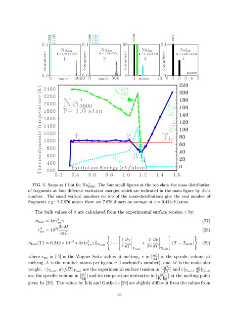
Figure 3: Atomic cluster fragmentation in the convex region of $S(E)$. The backbending caloric curve $T(E)$ (blue in the color version), left scale. The number of fragments $N_{fr}$ and the number of surface atoms $N_{eff}^{2/3}=\sum_{N_{i}\geq 2}N_{i}^{2/3}$ of larger fragments (green in the color version) can be read off from the right scale. $T_{tr}$ is the ”Maxwell” line dividing $T(E)$ into two equal area parts. The inserts above give the mass distribution at the various points along the caloric curve $T(E)$. The label ”4:1.295” means 1.295 quadrimers on average. This gives a detailed insight into what happens with rising excitation energy over the transition (convex) region: At the beginning ($e^{*}\sim 0.442$ eV) the liquid sodium drop evaporates 329 single atoms and 7.876 dimers and 1.295 quadrimers on average. At energies $e>\sim 1$eV the drop starts to fragment into several small droplets (”intermediate mass fragments”) e.g. at point 3: 2726 monomers, 80 dimers, $\sim$5 trimers, $\sim$15 quadrimers and a few heavier ones up to 10-mers. The evaporation residue disappears. This multifragmentation finishes at point 4. It induces the strong backward swing of the caloric curve $T(E)$. Above point 4 one has a gas of free monomers and at the beginning a few dimers. This transition scenario has a lot similarity with nuclear multifragmentation. It is also shown how the total interphase surface area, proportional to $N_{eff}^{2/3}=\sum_{i}N_{i}^{2/3}$ with $N_{i}\geq 2$ ($N_{i}$ the number of atoms in the $i$th cluster) stays almost constant up to point 3 even though the number of fragments ($N_{fr}=\sum_{i}$) is monotonic rising with increasing excitation.

In fig.3 I show the simulation of a typical fragmentation transition of a system of $3000$ sodium atoms interacting by realistic (many-body) forces. To compare with usual macroscopic conditions, the calculations were done at each energy using a volume $V(E)$ such that the microcanonical pressure $P=\frac{\partial S}{\partial V}/\frac{\partial S}{\partial E}=1$atm. Evidently, the convex region of $S(E,P)$ is the most interesting region.

3.3 Stars

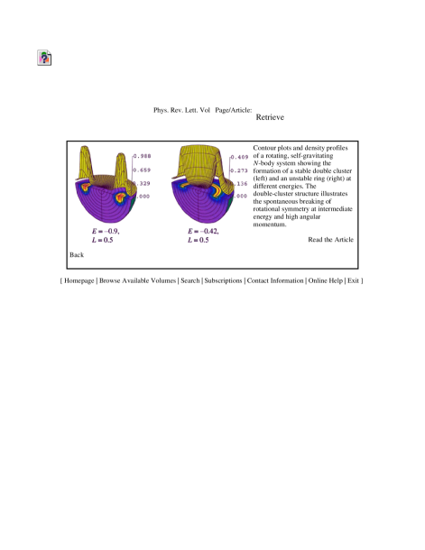
Figure 5: Phases and Phase-Separation in Rotating, Self-Gravitating Systems, Physical Review Letters–July 15, 2002, cover-page, by (Votyakov, Hidmi, De Martino, Gross)

Self-gravitation leads to a non-extensive potential energy $\propto N^{2}$. No thermodynamic limit exists for $E/N$ and no canonical treatment makes sense. At negative total energies often these systems have a negative heat capacity. This was for a long time considered as an absurd situation within canonical statistical mechanics with its thermodynamic “limit”. However, within our geometric theory this is just a simple example of the pseudo-Riemannian topology of the microcanonical entropy $S(E,N)$ provided that high densities with their non-gravitational physics, like nuclear hydrogen burning, are excluded. We treated the various phases of a self-gravitating cloud of particles as function of the total energy and angular momentum, c.f. fig.5 and the quoted PRL-paper. Clearly these are the most important constraint in astrophysics. In fig.6 the global phase diagram of a rotating, selfgravitating hydrogen cloud is given.

4 Conclusion

Entropy has a simple and elementary definition by the area $e^{S(E,N,\cdots)}$ of the microcanonical ensemble in the $6N$ dim. phase space. Canonical ensembles are not equivalent to the micro-ensemble in the most interesting situations:

1. At phase-separation ($\longrightarrow$heat engines !), one gets inhomogeneities, and a negative heat capacity or some other negative susceptibility, consequently:

2. Heat can flow from cold to hot.

3. Phase transitions can be localized sharply and unambiguously in small classical or quantum systems, there is no need for finite size scaling to identify the transition.

4. Also really large self-gravitating systems can be addressed.

Entropy rises during the approach to equilibrium, $\Delta S\geq 0$, also for small mixing systems. i.e. the Second Law is valid even if the Poincaré recurrence time is not astronomically large gross183 ; gross192 ; gross174 ; gross189 .

With this geometric foundation thermo-statistics applies not only to extensive systems but also to non-extensive ones which have no thermodynamic limit. More details are discussed in the references, see also my WEB-page http://www.hmi.de/people/gross/.

5 Acknowledgement

The author is grateful to A.Dellafiore, F.Matera, M. Pettini, and the members of the physics department of Florence, but especially to S.Ruffo, for many helpful discussions and their warm hospitality. He also acknowledges the financial support by the INFN and the University of Florence.

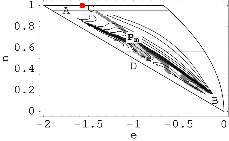
Figure 1: Global phase diagram or contour plot of the curvature determinant (Hessian) for a small system, eqn. (4), of the 2-dim Potts-3 lattice gas with $50*50$ lattice points, $n$ is the number of particles per lattice point, $e$ is the total energy per lattice point. The line (-2,1) to (0,0) is the ground-state energy of the lattice-gas as function of $n$. The most right curve is the locus of configurations with completely random spin-orientations (maximum entropy). The whole physics of the model plays between these two boundaries. The different regions of positive or negative Hessian, i.e. of respectively negative or positive maximum curvature $\lambda_{1}$ correspond to different phases (in the case studied here $\lambda_{2}$ is everywhere negative): At the dark-gray (green in the color version) lines the Hessian is $\det=0$, this is the boundary of the region of phase separation (the triangle $AP_{m}B$) with a negative Hessian ($\lambda_{1}>0,\lambda_{2}<0$). Here, we have Pseudo-Riemannian geometry and a convex entropy. At the light-gray (blue in the color version) lines is a minimum of $\det(e,n)$ in the direction of the largest curvature (v${}_{\lambda_{1}}\cdot$$\nabla$$\det=0$) and additionally $\det\approx 0$, these are lines of second order transition. In the triangle $AP_{m}C$ is the pure ordered (solid) phase with concave entropy and ($\det>0,\lambda_{1}<0,\lambda_{2}<0$). Above and right of the line $CP_{m}B$ is the pure disordered (gas) phase again with concave $s(e,n)$ and ($\det>0,\lambda_{1}<0,\lambda_{2}<0$). The crossing $P_{m}$ of the boundary lines is a multi-critical point. Here we have simultaneously $\lambda_{1}=0,$$\nabla$$\lambda_{1}=0$. It is also the critical end-point of the region of phase separation. The lighter-gray (red in the color version) region around the multi-critical point $P_{m}$ corresponds to a flat, horizontal region of $\det(e,n),\lambda_{1}\sim 0$ and consequently to a somewhat extended cylindrical region of $s(e,n)$, see gross174 ; gross173 ; $C$ (red) is the analytically known position of the critical point (second order transition) which the ordinary $q=3$ Potts model (without vacancies) would have in the thermodynamic limit. $C$ is also approached by the line of second-order transition (light-gray/blue) in the present small system.

Figure 2: The physical origin of convex regions in $S(E)$ for systems with interactions of short range. MMMC gross174 simulation of the entropy $s(e)$ per atom ($e$ in eV per atom) of a system of $N_{0}=1000$ sodium atoms at an external pressure of 1 atm. At the energy $e\leq e_{1}$ the system is in the pure liquid phase and at $e\geq e_{3}$ in the pure gas phase, of course with fluctuations which are proportional to the inverse negative curvature of $s(e)$. The latent heat per atom is $q_{lat}=e_{3}-e_{1}$. Attention: the curve $s(e)$ is artifically sheared by subtracting a linear function $25+e*11.5$ in order to make the convex intruder visible. $s(e)$ is always a steeply monotonic rising function. We clearly see the global concave (downwards bending) nature of $s(e)$ and its convex intruder. Its depth is the relative entropy loss due to additional correlations by internal interfaces. It scales $\propto N^{-1/3}$. From this one can calculate the surface tension per surface atom $\sigma_{surf}/T_{tr}=\Delta s_{surf}*N_{0}/N_{surf}$. For the present example it is $\sigma_{surf}/T_{tr}=5.68$ which should be compared to $\sigma_{surf}/T_{tr}=9.267$ for the bulk. The bulk value is approximated by $\sigma_{surf}/T_{tr}$ systematically with rising number of atoms $N$ [more details c.f.gross174 ; gross189 ]. The double tangent (Gibbs construction) is the concave hull of $s(e)$. Its derivative gives the Maxwell line in the caloric curve $T(e)$ at $T_{tr}$. In the thermodynamic limit the intruder would disappear and $s(e)$ would approach the double tangent from below. Nevertheless, even there, the probability $\propto e^{Ns}$ of configurations with phase-separations are suppressed by the (infinitesimal small) factor $e^{-N^{2/3}}$ relative to the pure phases and the distribution remains strictly bimodal in the canonical ensemble. The region $e_{1}<e<e_{3}$ of phase separation gets lost.

Figure 4: Heat can flow from hot to cold. Potts model (here with $q=10$ showing a strong first order transition), in the region of phase separation. At $e_{1}$ the system is in the pure ordered phase, at $e_{3}$ in the pure disordered phase. A little above $e_{1}$ the temperature $T=1/\beta$ is higher than a little below $e_{3}$. Combining two parts of the system: one at the energy $e_{1}+\delta e$ and at the temperature $T_{1}$, the other at the energy $e_{3}-\delta e$ and temperature $T_{3}<T_{1}$. It will equilibrize with a rise of its entropy, under a dropping of $T_{1}$ (cooling) and an energy flow (heat) from $3\to 1$: i.e.: Heat flows from cold to hot! Clausius formulation of the Second Law is violated. Evidently, this is not any peculiarity of gravitating systems! This is a generic situation within classical thermodynamics even for short-range coupling. It has nothing to do with long range interactions

.

Figure 6: Microcanonical global phase-diagram of a cloud of self-gravitating and rotating system in a spherical container as function of energy and angular-momentum. In this mean-field calculation local densities higher than the density where nuclear hydrogen burning starts are excluded. Thus, the gravitational collapse to only visible stars is followed. Outside the dashed boundaries only some singular points were calculated (e.g. see also previous figure). In the mixed phase the largest curvature $\lambda_{1}$ of $S(E,L)$ is positive. Consequently the heat capacity or the correspondent susceptibility is negative. This is of course well known in astrophysics. However, the new and important point of our finding is that within microcanonical thermodynamics this is a generic property of all phase transitions of first order, independently of whether there is a short- or a long-range force that organizes the system. The importance of using the microcanonical ensemble with angular momentum as the second control parameter cannot be overemphasized: The kinetic, ”chaotic energy” $E_{kin}=E-E_{pot}-L^{2}/2I$ is maximized at large moment of inertia $I$. Similar equilibrium calculations are done in astro-physics with angular velocity $\Omega=L/I$ as control parameter ($\sim$ canonical ensemble on the rotating disk), whence $E_{kin}=E-E_{pot}-I\times\Omega^{2}/2$. Then of course, the maximum of the entropy is at small moment of inertia and only mono-stars are found.

References

(1)
I. Pitowsky
Local Fluctuations and Local Observers in Equilibrium Statistical Mechanics
Studies in the History and Philosophy of Modern Physics,32:595-607,2001.
(2)
D.H.E. Gross.
Ensemble probabilistic equilibrium and non-equilibrium thermodynamics
without the thermodynamic limit.
In Andrei Khrennikov, editor, Foundations of Probability and
Physics, number XIII in PQ-QP: Quantum Probability, White Noise Analysis,
pages 131–146, Boston, October 2001. ACM, World Scientific.
(3)
D.H.E. Gross.
Second law in classical non-extensive systems.
In D. Sheehan, editor, Proceedings of the First International
Conference on Quantum Limits to the Second Law, pages cond–mat/0209467,
University of San Diego, 2002.
(4)
D.H.E. Gross.
Microcanonical thermodynamics: Phase transitions in “Small”
systems, volume 66 of Lecture Notes in Physics.
World Scientific, Singapore, 2001.
(5)
D.H.E. Gross.
Thermo-statistics or topology of the microcanonical entropy surface.
In T.Dauxois, S.Ruffo, E.Arimondo, and M.Wilkens, editors, Dynamics and Thermodynamics of Systems with Long Range Interactions, Lecture
Notes in Physics, 602, pages 21–45,cond–mat/0206341, Heidelberg, 2002.
Springer.
(6)
D.H.E. Gross and E. Votyakov.
Phase transitions in ”Small” systems.
Eur.Phys.J.B, 15:115–126, (2000),
http://arXiv.org/abs/cond-mat/?9911257.