Collective oscillations of a confined Bose gas at finite temperature in the random-phase approximation

Abstract

We present a theory for the linear dynamics of a weakly interacting Bose gas confined inside a harmonic trap at finite temperature. The theory treats the motions of the condensate and of the non-condensate on an equal footing within a generalized random-phase approximation, which (i) extends the second-order Beliaev-Popov approach by allowing for the dynamical coupling between fluctuations in the thermal cloud, and (ii) reduces to an earlier random-phase scheme when the anomalous density fluctuations are omitted. Numerical calculations of the low-lying spectra in the case of isotropic confinement show that the present theory obeys with high accuracy the generalized Kohn theorem for the dipolar excitations and demonstrate that combined normal and anomalous density fluctuations play an important role in the monopolar excitations of the condensate. Mean-field theory is instead found to yield accurate results for the quadrupolar modes of the condensate. Although the restriction to spherical confinement prevents quantitative comparisons with measured spectra, it appears that the non-mean field effects that we examine may be relevant to explain the features exhibited by the breathing mode as a function of temperature in the experiments carried out at JILA on a gas of ⁸⁷Rb atoms.

I Introduction

Soon after the realization of Bose-Einstein condensation in trapped atomic gases, an important development in this field has been the measurement of the frequencies and damping rates of collective excitations jin96 ; jin97 ; ketterle96 ; ketterle98 ; ketterle00 . These measurements are very accurate and provide a unique opportunity for quantitative tests of quantum theories of the dynamics of many-body systems. In particular, the measurements of the lowest-energy excitations made at JILA jin97 on ⁸⁷Rb gases at various temperatures have proved hard to understand at simple mean-field level burnett ; hutchinson and have therefore stimulated a number of theoretical studies to address effects beyond the mean-field approximation overview ; fs ; giorgini ; morgan00 ; morgan03 ; reidl00 ; stoof ; zgn ; mt .

The key issue in investigations transcending the mean-field level is the full dynamic description of both condensed and non-condensed atoms and their mutual interactions mt . While the condensate dynamics is well described by a single nonlinear Gross-Pitaevskii equation (GPE), how to monitor the evolution of the non-condensate is a much more delicate problem. The best candidate theory that takes into account the coupled dynamics of condensate and non-condensate for a homogeneous weakly-interacting Bose gas in the collisionless limit is the second-order Beliaev-Popov (SOBP) theory beliaev , which has been reexamined recently by Shi and Griffin griffin98 and extended to trapped gases by Fedichev and Shlyapnikov fs and by Giorgini giorgini (see also Rusch et al. morgan00 ). However, for the trapped gas the Thomas-Fermi approximation on the SOBP theory fails to account for the JILA observations fs ; giorgini . One possible reason is that the dynamics of the condensate and non-condensate are not treated on an equal footing in the theory, i.e. the dynamical coupling between fluctuations in the thermal cloud is not included. This coupling should be important when the thermal fraction is significantly populated and, as will be discussed below, is in fact needed to satisfy the generalized Kohn theorem for the dipole modes. One way to include these processes is to use the linear response theory in the random-phase approximation (RPA) as developed by two of us mt . Such a treatment chooses the Hartree-Fock gas as the reference system for the thermal atoms, thus neglecting the anomalous density fluctuations that may play a role at intermediate temperatures.

In the present paper we improve on the Hartree-Fock RPA (HF-RPA) by including the anomalous density fluctuations. The resulting theory can be referred to as the HFB-RPA since our choice of the reference system is provided by the first-order Hartree-Fock-Bogoliubov theory. We explicitly show that the HFB-RPA theory formally reduces to the SOBP theory given by Fedichev and Shlyapnikov fs and by Giorgini giorgini if (i) one excludes the process of driving the non-condensate by its self-generated dynamical potential, and (ii) one keeps only terms of second order in the coupling constant. It is interesting to note that the HF-RPA similarly reduces to the dielectric formalism given by Reidl et al. reidl00 .

We then numerically investigate the low-lying excitations of a fluid representing a Bose-condensed gas of 2000 ⁸⁷Rb atoms in a spherically symmetric harmonic trap at finite temperature by using the HFB-RPA as well as the SOBP theory and the HF-RPA. All three theories give qualitatively the same results for the quadrupolar mode of the condensate. However they predict different trends for the monopolar mode, due to the strong coupling between the oscillations of the condensate and those of the non-condensate. For the first time this observation highlights the crucial roles played already in the linear excitation spectra by the normal and anomalous density fluctuations of the non-condensate.

The paper is organized as follows. In Sec. II we derive the generalized RPA equations within the framework of the Hartree-Fock-Bogoliubov approximation, and in Sec. III we briefly demonstrate how to deduce the SOBP theory from the HFB-RPA equations. In Sec. IV we describe our numerical procedure for calculating the spectral response functions and check their accuracy, and in Secs. V and VI we present our numerical results for the low-energy excitations. Finally, Sec. VII presents our main conclusions.

II The HFB-RPA theory

The essential idea of the RPA is that the gas responds as a reference gas to self-consistent dynamical potentials overview . In the HF-RPA treatment one chooses as dynamical variables the density fluctuations $\delta n_{c}$ of the condensate and $\delta\tilde{n}$ of the non-condensate mt . The HF-RPA equations follow by imposing that the condensed and non-condensed particles experience dynamical Hartree-Fock potentials generated by both types of density fluctuations and respond to them as a Hartree-Fock gas.

Our starting point for the derivation of the HFB-RPA is the definition of the appropriate single-particle reference system. The contribution of the anomalous density is included by choosing the Hartree-Fock-Bogoliubov gas at finite temperature as reference, which is defined in terms of the condensate wavefunction $\Phi_{0}$ and of the single-particle amplitudes $u_{j}$ and $v_{j}$ for the non-condensate griffin96 . The condensate is described by the generalized GPE

$$\left[-\frac{\hbar^{2}\mathbf{\bigtriangledown}^{2}}{2m}+V_{ext}\left(\mathbf{r}\right)+g\left(n_{c}\left(\mathbf{r}\right)+2\tilde{n}^{0}\left(\mathbf{r}\right)\right)\right]\Phi_{0}\left(\mathbf{r}\right)+g\tilde{m}^{0}\left(\mathbf{r}\right)\Phi_{0}^{*}\left(\mathbf{r}\right)=\mu\Phi_{0}\left(\mathbf{r}\right),$$ (1)

where we adopt the standard contact-pseudopotential model characterized by the coupling constant $g=4\pi\hbar^{2}a/m$, with $a$ being the s-wave scattering length. In Eq. (1) $V_{ext}\left(\mathbf{r}\right)=m(\omega_{x}^{2}x^{2}+\omega_{y}^{2}y^{2}+\omega_{z}^{2}z^{2})/2$ is the external confinement and $n_{c}\left(\mathbf{r}\right)=\left|\Phi_{0}\left(\mathbf{r}\right)\right|^{2}$, $\tilde{n}^{0}\left(\mathbf{r}\right)=\sum_{j}\left[\left(\left|u_{j}\left(\mathbf{r}\right)\right|^{2}+\left|v_{j}\left(\mathbf{r}\right)\right|^{2}\right)f_{j}+\left|v_{j}\left(\mathbf{r}\right)\right|^{2}\right]$, and $\tilde{m}^{0}\left(\mathbf{r}\right)=$ $\sum_{j}\left[\left(1+2f_{j}\right)u_{j}\left(\mathbf{r}\right)v_{j}^{*}\left(\mathbf{r}\right)\right]$ are the condensate density and the normal and anomalous thermal densities, $f_{j}=1/\left(e^{\beta\epsilon_{j}}-1\right)$ being the Bose-Einstein distribution with $\beta=1/k_{B}T$ and $\mu$ the chemical potential. The non-condensate amplitudes are obtained by the solution of the generalized Bogoliubov-deGennes equations

$$\left\{\begin{array}[]{l}\mathcal{L}\left(\mathbf{r}\right)u_{j}\left(\mathbf{r}\right)+g\left(\Phi_{0}^{2}\left(\mathbf{r}\right)+\tilde{m}^{0}\left(\mathbf{r}\right)\right)v_{j}\left(\mathbf{r}\right)=\epsilon_{j}u_{j}\left(\mathbf{r}\right)\\ \mathcal{L}\left(\mathbf{r}\right)v_{j}\left(\mathbf{r}\right)+g\left(\Phi_{0}^{*2}\left(\mathbf{r}\right)+\tilde{m}^{0*}\left(\mathbf{r}\right)\right)u_{j}\left(\mathbf{r}\right)=-\epsilon_{j}v_{j}\left(\mathbf{r}\right).\end{array}\right.$$ (2)

Here $\mathcal{L}\left(\mathbf{r}\right)=-\hbar^{2}\mathbf{\bigtriangledown}^{2}/2m+V_{ext}\left(\mathbf{r}\right)+2g\left(n_{c}\left(\mathbf{r}\right)+\tilde{n}^{0}\left(\mathbf{r}\right)\right)$. The Popov approximation to the Hartree-Fock-Bogoliubov (HFB-Popov) theory is recovered by setting $\tilde{m}^{0}\left(\mathbf{r}\right)=0$ in Eqs. (1) and (2) griffin96 .

We would like to remark that from a dynamical point of view the amplitudes $u_{j}$ and $v_{j}$ can alternatively be viewed as excitations out of the condensate. The duality of such mean-field description follows from the assumption of Bose symmetry breaking (see e.g. rmp for a discussion).

In deriving next the HFB-RPA equations we adopt five dynamic variables, which are the fluctuations $\delta\Phi$ and $\delta\Phi^{*}$ of the condensate wavefunction and its complex conjugate, the normal density fluctuation $\delta\tilde{n}$, and the anomalous density fluctuation $\delta\tilde{m}$ together with its complex conjugate $\delta\tilde{m}^{*}$. $\delta\Phi$ and $\delta\Phi^{*}$ are separately introduced because of their different coupling to $\delta\tilde{m}$ and $\delta\tilde{m}^{*}$, and are related to the density fluctuation of the condensate by $\delta n_{c}=\Phi_{0}^{*}\delta\Phi+\Phi_{0}\delta\Phi^{*}$. The HFB-RPA then follows naturally by evaluating the self-consistent dynamical Hartree-Fock-Bogoliubov potential generated by the density fluctuations of the condensate (phonon quasiparticles) and of the non-condensate (thermal quasiparticles). This can be done by invoking the decomposition

$$\psi\left(\mathbf{r},t\right)=\Phi_{0}\left(\mathbf{r}\right)+\tilde{\psi}\left(\mathbf{r},t\right)$$ (3)

for the Bose field operator in the interaction Hamiltonian,

$$\mathcal{H}_{int} = \frac{g}{2}\int d\mathbf{r}\psi^{+}\left(\mathbf{r},t\right)\psi^{+}\left(\mathbf{r},t\right)\psi\left(\mathbf{r},t\right)\psi\left(\mathbf{r},t\right)$$ (4)

$$= \frac{g}{2}\int d\mathbf{r}\left[\left|\Phi_{0}\right|^{4}+2\left|\Phi_{0}\right|^{2}\Phi_{0}^{*}\tilde{\psi}+2\left|\Phi_{0}\right|^{2}\Phi_{0}\tilde{\psi}^{+}\right.$$

$$\left.+\Phi_{0}^{*}\Phi_{0}^{*}\tilde{\psi}\tilde{\psi}+4\left|\Phi_{0}\right|^{2}\tilde{\psi}^{+}\tilde{\psi}+\Phi_{0}\Phi_{0}\tilde{\psi}^{+}\tilde{\psi}^{+}\right.$$

$$\left.+2\Phi_{0}^{*}\tilde{\psi}^{+}\tilde{\psi}\tilde{\psi}+2\Phi_{0}\tilde{\psi}^{+}\tilde{\psi}^{+}\tilde{\psi}+\tilde{\psi}^{+}\tilde{\psi}^{+}\tilde{\psi}\tilde{\psi}\right]\text{.}$$

Note that in the choice made in Eq. (3), which is different from those generally used in the literature, the non-equilibrium statistical average $\left\langle\tilde{\psi}\left(\mathbf{r},t\right)\right\rangle$ of the operator $\tilde{\psi}\left(\mathbf{r},t\right)$ is non-zero since we prefer to extract from $\psi\left(\mathbf{r},t\right)$ a time-independent condensate wavefunction. Rather, $\tilde{\psi}\left(\mathbf{r},t\right)$ gives the field operator for the phonon quasiparticles and describes the condensate fluctuation, $\left\langle\tilde{\psi}\left(\mathbf{r},t\right)\right\rangle=\left\langle\psi\left(\mathbf{r},t\right)\right\rangle-\Phi_{0}\left(\mathbf{r}\right)=\Phi\left(\mathbf{r},t\right)-\Phi_{0}\left(\mathbf{r}\right)=\delta\Phi\left(\mathbf{r},t\right).$ Analogously $\delta\Phi^{*}\left(\mathbf{r},t\right)=\left\langle\psi^{+}\left(\mathbf{r},t\right)\right\rangle-\Phi_{0}^{*}\left(\mathbf{r}\right)$.

The self-consistent dynamical potentials are originated from the higher-order correlation terms beyond the mean-field description and are contained in the last line of Eq. (4). We approximate these terms by using Wick’s theorem in the following manner:

$$2\Phi_{0}^{*}\tilde{\psi}^{+}\tilde{\psi}\tilde{\psi} \simeq 4\Phi_{0}^{*}\left\langle\tilde{\psi}^{+}\tilde{\psi}\right\rangle\tilde{\psi}+2\Phi_{0}^{*}\left\langle\tilde{\psi}\tilde{\psi}\right\rangle\tilde{\psi}^{+}+4\Phi_{0}^{*}\delta\Phi\tilde{\psi}^{+}\tilde{\psi}+2\Phi_{0}^{*}\delta\Phi^{*}\tilde{\psi}\tilde{\psi},$$ (5)

$$2\Phi_{0}\tilde{\psi}^{+}\tilde{\psi}^{+}\tilde{\psi} \simeq 4\Phi_{0}\left\langle\tilde{\psi}^{+}\tilde{\psi}\right\rangle\tilde{\psi}^{+}+2\Phi_{0}\left\langle\tilde{\psi}^{+}\tilde{\psi}^{+}\right\rangle\tilde{\psi}+4\Phi_{0}\delta\Phi^{*}\tilde{\psi}^{+}\tilde{\psi}+2\Phi_{0}\delta\Phi\tilde{\psi}^{+}\tilde{\psi}^{+}$$ (6)

and

$$\tilde{\psi}^{+}\tilde{\psi}^{+}\tilde{\psi}\tilde{\psi}\simeq 4\left\langle\tilde{\psi}^{+}\tilde{\psi}\right\rangle\tilde{\psi}^{+}\tilde{\psi}+\left\langle\tilde{\psi}^{+}\tilde{\psi}^{+}\right\rangle\tilde{\psi}\tilde{\psi}+\left\langle\tilde{\psi}\tilde{\psi}\right\rangle\tilde{\psi}^{+}\tilde{\psi}^{+}.$$ (7)

Explicitly, the fluctuations of the non-condensate are defined by $\delta\tilde{n}\left(\mathbf{r},t\right)=\left\langle\psi^{+}\left(\mathbf{r},t\right)\psi\left(\mathbf{r},t\right)\right\rangle-\tilde{n}^{0}\left(\mathbf{r}\right)$, $\delta\tilde{m}\left(\mathbf{r},t\right)=\left\langle\psi\left(\mathbf{r},t\right)\psi\left(\mathbf{r},t\right)\right\rangle-\tilde{m}^{0}\left(\mathbf{r}\right)$, and $\delta\tilde{m}^{*}\left(\mathbf{r},t\right)=\left\langle\psi^{+}\left(\mathbf{r},t\right)\psi^{+}\left(\mathbf{r},t\right)\right\rangle-\tilde{m}^{0*}\left(\mathbf{r}\right)$. We insert these definitions into Eqs. (5)-(7), remove the terms that are proportional to $\tilde{n}^{0}\left(\mathbf{r}\right)$, $\tilde{m}^{0}\left(\mathbf{r}\right)$ and $\tilde{m}^{0*}\left(\mathbf{r}\right)$ as these are already accounted by the Hartree-Fock-Bogoliubov mean-field equations, and finally collect together the remaining terms. We then find that the self-consistent dynamical potential induced by fluctuations is

$$\mathcal{\delta V}^{SC} = g\int d\mathbf{r}\left[2\Phi_{0}^{*}\delta\tilde{n}\tilde{\psi}+\Phi_{0}^{*}\delta\tilde{m}\tilde{\psi}^{+}+2\Phi_{0}\delta\tilde{n}\tilde{\psi}^{+}+\Phi_{0}\delta\tilde{m}^{*}\tilde{\psi}\right.$$ (8)

$$\left.+2\Phi_{0}^{*}\delta\Phi\tilde{\psi}^{+}\tilde{\psi}+\Phi_{0}^{*}\delta\Phi^{*}\tilde{\psi}\tilde{\psi}+2\Phi_{0}\delta\Phi^{*}\tilde{\psi}^{+}\tilde{\psi}+\Phi_{0}\delta\Phi\tilde{\psi}^{+}\tilde{\psi}^{+}\right.$$

$$\left.+2\delta\tilde{n}\tilde{\psi}^{+}\tilde{\psi}+\delta\tilde{m}\tilde{\psi}^{+}\tilde{\psi}^{+}/2+\delta\tilde{m}^{*}\tilde{\psi}\tilde{\psi}/2\right]\text{.}$$

Physically, the eight leading terms on the right-hand side of Eq. (8) are the self-consistent potentials generated by phonon quasiparticles on themselves and on thermal quasiparticles. These terms have been discussed by Giorgini giorgini and by Liu and Hu liu and, as we shall see explicitly below, lead to the SOBP theory in a perturbative treatment to second order in the coupling constant. On the other hand, the last three terms in Eq. (8) describe the self-potential of the thermal quasiparticles and are expected to excite zero-sound-like collective modes of the non-condensate. Although these terms are only of third order in the coupling constant and therefore are missing in the SOBP theory, they may have a significant role when the depletion of the condensate is large. They are also required for consistency with the generalized Kohn theorem.

With the self-consistent Hartree-Fock-Bogoliubov potential in Eq. (8) and using the notation $\chi f\equiv\int d\mathbf{r}^{\prime}\chi\left(\mathbf{r},\mathbf{r}^{\prime},\omega\right)f(\mathbf{r}^{\prime})$, we can write the coupled HFB-RPA equations for $\delta\Phi$, $\delta\Phi^{*}$, $\delta\tilde{n}$, $\delta\tilde{m}$ and $\delta\tilde{m}^{*}$ in a compact matrix form. Within the linear response framework we have

$$\left(\begin{array}[]{c}\delta\Phi\\ \delta\Phi^{*}\end{array}\right)=g\left(\begin{array}[]{cc}\chi_{cc}&\chi_{c\bar{c}}\\ \chi_{\bar{c}c}&\chi_{\bar{c}\bar{c}}\end{array}\right)\left(\begin{array}[]{c}2\Phi_{0}^{*}\delta\tilde{n}+\Phi_{0}\delta\tilde{m}^{*}\\ 2\Phi_{0}\delta\tilde{n}+\Phi_{0}^{*}\delta\tilde{m}\end{array}\right)$$ (9)

and

$$\left(\begin{array}[]{c}\delta\tilde{n}\\ \delta\tilde{m}\\ \delta\tilde{m}^{*}\end{array}\right)=g\left(\begin{array}[]{ccc}\chi_{\tilde{n}\tilde{n}}&\chi_{\tilde{n}\tilde{m}}&\chi_{\tilde{n}\tilde{m}^{+}}\\ \chi_{\tilde{m}\tilde{n}}&\chi_{\tilde{m}\tilde{m}}&\chi_{\tilde{m}\tilde{m}^{+}}\\ \chi_{\tilde{m}^{+}\tilde{n}}&\chi_{\tilde{m}^{+}\tilde{m}}&\chi_{\tilde{m}^{+}\tilde{m}^{+}}\end{array}\right)\left(\begin{array}[]{c}2\Phi_{0}^{*}\delta\Phi+2\Phi_{0}\delta\Phi^{*}+2\delta\tilde{n}\\ \Phi_{0}^{*}\delta\Phi^{*}+\delta\tilde{m}^{*}/2\\ \Phi_{0}\delta\Phi+\delta\tilde{m}/2\end{array}\right).$$ (10)

In these equations $\chi_{\alpha\beta}$ ($\alpha$, $\beta=c$ or $\bar{c}$ ) and $\chi_{ab}$ ($a$, $b=\tilde{n}$, $\tilde{m}$, or $\tilde{m}^{+}$) are the two-particle response functions of the condensate and non-condensate components, respectively. They can easily be evaluated by using the quasiparticle amplitudes obtained from the Hartree-Fock-Bogoliubov solutions in the standard finite-temperature Green’s functions technique fetter . For the condensate we have

$$\chi_{cc}\left(\mathbf{r},\mathbf{r}^{\prime},\omega\right) = \sum_{j}\left(\frac{u_{j}\left(\mathbf{r}\right)v_{j}^{*}\left(\mathbf{r}^{\prime}\right)}{\hbar\omega^{+}-\epsilon_{j}}-\frac{v_{j}^{*}\left(\mathbf{r}\right)u_{j}\left(\mathbf{r}^{\prime}\right)}{\hbar\omega^{+}+\epsilon_{j}}\right),$$ (11)

$$\chi_{c\bar{c}}\left(\mathbf{r},\mathbf{r}^{\prime},\omega\right) = \sum_{j}\left(\frac{u_{j}\left(\mathbf{r}\right)u_{j}^{*}\left(\mathbf{r}^{\prime}\right)}{\hbar\omega^{+}-\epsilon_{j}}-\frac{v_{j}^{*}\left(\mathbf{r}\right)v_{j}\left(\mathbf{r}^{\prime}\right)}{\hbar\omega^{+}+\epsilon_{j}}\right),$$ (12)

$$\chi_{\bar{c}c}\left(\mathbf{r},\mathbf{r}^{\prime},\omega\right) = \sum_{j}\left(\frac{v_{j}\left(\mathbf{r}\right)v_{j}^{*}\left(\mathbf{r}^{\prime}\right)}{\hbar\omega^{+}-\epsilon_{j}}-\frac{u_{j}^{*}\left(\mathbf{r}\right)u_{j}\left(\mathbf{r}^{\prime}\right)}{\hbar\omega^{+}+\epsilon_{j}}\right)$$ (13)

and

$$\chi_{\bar{c}\bar{c}}\left(\mathbf{r},\mathbf{r}^{\prime},\omega\right)=\sum_{j}\left(\frac{v_{j}\left(\mathbf{r}\right)u_{j}^{*}\left(\mathbf{r}^{\prime}\right)}{\hbar\omega^{+}-\epsilon_{j}}-\frac{u_{j}^{*}\left(\mathbf{r}\right)v_{j}\left(\mathbf{r}^{\prime}\right)}{\hbar\omega^{+}+\epsilon_{j}}\right),$$ (14)

where $\omega^{+}=\omega+i\eta$ with $\eta=0^{+}$. The expressions for the two-particle response functions of the non-condensate are lengthier and we list them in Appendix A.

The coupled HFB-RPA equations (9) and (10) are the central result of this work. They reduce to the HF-RPA equations if one omits the anomalous density fluctuations of thermal quasiparticles. That is, the HF-RPA gives

$$\delta n_{c}\left(\mathbf{r},\omega\right)=2g\int d\mathbf{r}^{\prime}\chi_{c}\left(\mathbf{r},\mathbf{r}^{\prime};\omega\right)\delta\tilde{n}(\mathbf{r}^{\prime},\omega)$$ (15)

and

$$\delta\tilde{n}\left(\mathbf{r},\omega\right)=2g\int d\mathbf{r}^{\prime}\chi_{\tilde{n}\tilde{n}}\left(\mathbf{r},\mathbf{r}^{\prime};\omega\right)\left[\delta n_{c}\left(\mathbf{r}^{\prime},\omega\right)+\delta\tilde{n}(\mathbf{r}^{\prime},\omega)\right],$$ (16)

where $\chi_{c}\left(\mathbf{r},\mathbf{r}^{\prime};\omega\right)=\Phi_{0}^{*}\left(\mathbf{r}\right)\chi_{cc}\Phi_{0}^{*}(\mathbf{r}^{\prime})+\Phi_{0}\left(\mathbf{r}\right)\chi_{\bar{c}c}\Phi_{0}^{*}(\mathbf{r}^{\prime})+\Phi_{0}^{*}\left(\mathbf{r}\right)\chi_{c\bar{c}}\Phi_{0}(\mathbf{r}^{\prime})+\Phi_{0}\left(\mathbf{r}\right)\chi_{\bar{c}\bar{c}}\Phi_{0}(\mathbf{r}^{\prime})$. One must accordingly take the Hartree-Fock reference system in the calculation of the response functions mt .

III Reduction to the second-order Beliaev-Popov theory

In this Section we show that the coupled HFB-RPA equations for the normal modes of the condensate simplify to those obtained in the SOBP theory if we neglect the self-coupling of density fluctuations in the non-condensate and keep only terms up to second order in the coupling constant $g$. This discussion also allows us to define a RPA form of the SOBP theory, that will later be used in our numerical calculations.

If we neglect the terms in $\delta\tilde{n}$, $\delta\tilde{m}$ and $\delta\tilde{m}^{*}$ on the right-hand side of Eq. (10) and substitute this equation in Eq. (9), we immediately obtain the self-consistent equations for the fluctuations of the condensate as

$$\left(\begin{array}[]{l}\delta\Phi\\ \delta\Phi^{*}\end{array}\right)=g^{2}\left(\begin{array}[]{cc}\chi_{cc}&\chi_{c\bar{c}}\\ \chi_{\bar{c}c}&\chi_{\bar{c}\bar{c}}\end{array}\right)\mathcal{D}\left(\begin{array}[]{l}\delta\Phi\\ \delta\Phi^{*}\end{array}\right),$$ (17)

where the matrix $\mathcal{D}$ is defined as

$$\mathcal{D}=\left(\begin{array}[]{lll}2\Phi_{0}^{*}&0&\Phi_{0}\\ 2\Phi_{0}&\Phi_{0}^{*}&0\end{array}\right)\left(\begin{array}[]{lll}\chi_{\tilde{n}\tilde{n}}&\chi_{\tilde{n}\tilde{m}}&\chi_{\tilde{n}\tilde{m}^{+}}\\ \chi_{\tilde{m}\tilde{n}}&\chi_{\tilde{m}\tilde{m}}&\chi_{\tilde{m}\tilde{m}^{+}}\\ \chi_{\tilde{m}^{+}\tilde{n}}&\chi_{\tilde{m}^{+}\tilde{m}}&\chi_{\tilde{m}^{+}\tilde{m}^{+}}\end{array}\right)\left(\begin{array}[]{ll}2\Phi_{0}^{*}&2\Phi_{0}\\ 0&\Phi_{0}^{*}\\ \Phi_{0}&0\end{array}\right).$$ (18)

Equation (17) is already of second order in $g$ and we shall regard it as providing a second-order Beliaev-Popov theory within a random-phase framework (SOBP-RPA).

The SOBP-RPA differs only slightly from the SOBP theory presented in Ref. giorgini , in the sense that it still keeps a class of terms beyond second order. In fact, to second order in the coupling constant we can describe the small oscillations of the condensate by a set $(u_{osc},v_{osc})$ of quasiparticle amplitudes with excitation energy $\epsilon_{osc}$. By setting $(\delta\Phi,\delta\Phi^{*})=(u_{osc},v_{osc})$ in Eq. (17) and using Eqs. (11)-(14) we find the eigenfrequency of the oscillations of the condensate as $\epsilon_{osc}+\delta E-i\gamma,$ where

$$\delta E-i\gamma = g^{2}\left(\begin{array}[]{ll}v_{osc}^{*},&u_{osc}^{*}\end{array}\right)\mathcal{D}\left(\begin{array}[]{l}u_{osc}\\ v_{osc}\end{array}\right)$$ (22)

$$= g\int d\mathbf{r}\Phi_{0}\left[2\left(u_{osc}^{*}+v_{osc}^{*}\right)\delta\tilde{n}+u_{osc}^{*}\delta\tilde{m}+v_{osc}^{*}\delta\tilde{m}^{*}\right].$$ (23)

In recent work two of us liu have explicitly shown that Eq. (23) agrees with the result for the eigenfrequency shift given by the SOBP theory of Giorgini giorgini .

IV Numerical procedure

We turn to numerical illustrations of the excitation spectra with the main aim of comparatively examining the three theoretical approaches that we have introduced in Secs. II and III. We do this in the case of a spherically symmetric trap in view of the complexity of the calculations involved.

We excite density fluctuations by applying a time-dependent perturbation of the form $F(t)\propto\exp\left(i\omega t\right)\int d\mathbf{r}V_{p}\left(\mathbf{r}\right)\psi^{+}\left(\mathbf{r}\right)\psi\left(\mathbf{r}\right)$. In the HFB-RPA this corresponds to adding the terms $\left[\begin{array}[]{ll}\chi_{cc}V_{p}\Phi_{0}^{*}+\chi_{c\bar{c}}V_{p}\Phi_{0},&\chi_{\bar{c}c}V_{p}\Phi_{0}^{*}+\chi_{\bar{c}\bar{c}}V_{p}\Phi_{0}\end{array}\right]^{T}$ and $\left[\begin{array}[]{lll}\chi_{\tilde{n}\tilde{n}}V_{p},&\chi_{\tilde{m}\tilde{n}}V_{p},&\chi_{\tilde{m}^{+}\tilde{n}}V_{p}\end{array}\right]^{T}$ on the right-hand side of Eqs. (9) and (10), respectively. The various density fluctuations are then calculated by the method of Capuzzi and Hernández capuzzi , with a discretization of the dynamical equations on a spatial mesh of up to 256 points. The frequencies of the collective excitations of the system can be extracted from the resonances of the spectral function $\chi^{{}^{\prime\prime}}\left(\omega\right)$, which is also the quantity of experimental interest. This is defined in the HFB-RPA as

$$\chi^{{}^{\prime\prime}}\left(\omega\right)=\chi_{C}^{{}^{\prime\prime}}\left(\omega\right)+\chi_{T}^{{}^{\prime\prime}}\left(\omega\right)$$ (24)

where

$$\chi_{C}^{{}^{\prime\prime}}\left(\omega\right)=-\frac{1}{\pi}Im\int d\mathbf{r}V_{p}(\mathbf{r})\left(\Phi_{0}^{*}\delta\Phi+\Phi_{0}\delta\Phi^{*}\right)$$ (25)

and

$$\chi_{T}^{{}^{\prime\prime}}\left(\omega\right)=-\frac{1}{\pi}Im\int d\mathbf{r}V_{p}(\mathbf{r})\left(\delta\tilde{n}+\delta\tilde{m}+\delta\tilde{m}^{*}\right).$$ (26)

Here the indices $C$ and $T$ refer to the contributions from the condensate and from the non-condensate. Other quantities of interest are the density fluctuations of the condensate and the non-condensate, which are readily extracted from the solution of Eqs. (9) and (10).

The main technical difficulty in the numerical calculations is how to renormalize the ultraviolet divergence caused by the use of contact interactions huang . The divergence appears in the equilibrium anomalous density $\tilde{m}^{0}\left(\mathbf{r}\right)$ and in the response functions $\chi_{\tilde{m}\tilde{m}^{+}}$ and $\chi_{\tilde{m}^{+}\tilde{m}}$. The simplest way to implement renormalization is by removing the zero-temperature component of the above quantities. This procedure is not fully correct as it neglects the quantum contributions hutchinson , but these are extremely small at temperatures where the thermal corrections become important. Alternatively one can apply renormalization by regularizing $\tilde{m}^{0}\left(\mathbf{r}\right)$, $\chi_{\tilde{m}\tilde{m}^{+}}$ and $\chi_{\tilde{m}^{+}\tilde{m}}$ in real space bruun . We have checked that these two procedures give almost the same mode frequencies in calculations based on the standard SOBP theory.

In brief, the numerical method that we have used consists of three steps. Firstly, we solve the HFB Eqs. (1) and (2) (or, in case of HF-RPA, the corresponding HF equations) to determine the equilibrium densities and quasiparticle amplitudes. We then construct the bare two-particle response functions and compute the dynamic fluctuations from Eqs. (9) and (10). We finally calculate the imaginary part of the response functions according to Eq. (24). In the present case of an isotropic trap, the calculations can be greatly simplified by projecting the RPA equations and the response functions onto the various multipole modes capuzzi . We shall be interested in the monopolar, dipolar, and quadrupolar excitations, which require setting $V_{p}\left(\mathbf{r}\right)\propto r^{2}$, $V_{p}\left(\mathbf{r}\right)\propto r\cos\theta$ and $V_{p}\left(\mathbf{r}\right)\propto r^{2}Y_{20}\left(\theta,\varphi\right)$.

In the following we evaluate a gas of $N=2000$ ⁸⁷Rb atoms in a spherical trap with trap frequency $\omega_{0}=2\pi\times 182.5$ Hz, this value being the geometric average of the axial and radial frequencies in the JILA experiments jin97 . The temperature is taken in units of the critical temperature for an ideal gas with the same value of $N$ and $\omega_{0}$, which is $T_{c}=0.94\hbar\omega_{0}N^{1/3}$. In most calculations we use a basis of $n\leq n_{\max}=24$ and $l\leq l_{\max}=32$ for the quasiparticle wavefunctions, where the indices $n$ and $l$ label the number of radial nodes and the orbital angular momentum of the wavefunction.

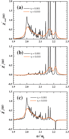
Figure 1: Spectral responses (in arbitrary units) for the monopolar excitation as functions of frequency $\omega$ (in units of $\omega_{0}$) as calculated from the HF-RPA at $T/T_{c}=0.5$, plotted for two values of $\eta$ (in units of $\omega_{0}$) as indicated in the panels. The three panels display the total spectral response (a) and the contributions of the condensate (b) and of the non-condensate (c).

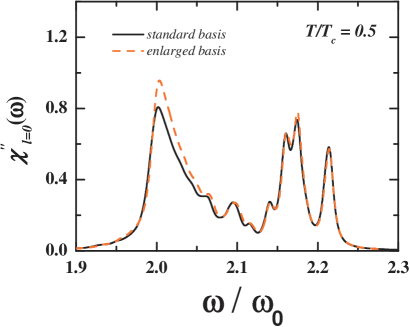
Figure 2: Spectral response (in arbitrary units) for the monopolar excitation as a function of frequency $\omega$ (in units of $\omega_{0}$) as calculated from the HF-RPA at $T/T_{c}=0.5$ and $\eta=0.005\omega_{0}$ with two kinds of basis set.

IV.1 Tests of numerical accuracy

In this subsection we report some tests of the accuracy of our numerical calculations. First of all, we must replace the positive infinitesimal quantity $\eta$ in the reference response functions by a finite value. In Fig. 1 we show the spectral functions for the monopolar excitation in the HF-RPA for two values of $\eta$ at a reduced temperature $T/T_{c}=0.5$. For small value of $\eta$ many spikes appear in the spectrum, due to the discrete basis set that was chosen for the dynamical description. With increasing $\eta$ these spikes are rounded off into broad resonances, which are insensitive to the precise value of $\eta$. In the following we preferentially take $\eta=0.01\omega_{0}$ in calculating the spectral functions, this choice being consistent with a typical experimental energy resolution jin97 .

The other aspect of the calculations that needs examining is the role of the basis set. In Fig. 2 we show the HF-RPA monopole spectrum at $T/T_{c}=0.6$ and $\eta=0.005\omega_{0}$, as calculated from two choices of basis set. These are the standard set as described above (solid line) and a set in which the number of basis function has been doubled (dashed line). No quantitative changes are found for the condensate response around $\omega=2.2\omega_{0}$, while for the response of the thermal cloud near $\omega=2.0\omega_{0}$ only a small change is present in the spectral intensity.

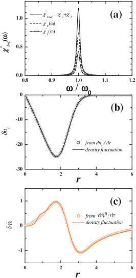
Figure 3: (a) Spectral response (in arbitrary units) for the dipolar excitation as a function of frequency $\omega$ (in units of $\omega_{0}$), as calculated from the HF-RPA at $T/T_{c}=0.6$ with the choice $\eta=0.005\omega_{0}$. The density fluctuations at resonance (in arbitrary units) are plotted as functions of the radial coordinate $r$ (in units of $a_{ho}=(\hbar/m\omega_{0})^{1/2}$) in (b) for the condensate and in (c) for the non-condensate (solid lines). In the same panels are also shown the corresponding results from the analytical expressions of the mode eigenvectors (circles).

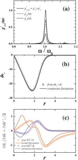
Figure 4: The same as Fig. 3 for the HFB-RPA.

V Dipole mode

An important check on the accuracy of the theory is offered by the Kohn theorem. One can analytically prove that the dipolar oscillation in the $\alpha$ direction (with $\alpha=x$, $y$, or $z$ in the general case of an anisotropic trap) is described by the Ansatz $\delta\Phi=\left(\partial/\partial r_{\alpha}-mr_{\alpha}\omega_{\alpha}/\hbar\right)\Phi_{0}$, $\delta\Phi^{*}=\left(\partial/\partial r_{\alpha}+mr_{\alpha}\omega_{\alpha}/\hbar\right)\Phi_{0}^{*}$, $\delta\tilde{n}=\partial\tilde{n}^{0}/\partial r_{\alpha}$, $\delta\tilde{m}=\left(\partial/\partial r_{\alpha}-2mr_{\alpha}\omega_{\alpha}/\hbar\right)\tilde{m}^{0}$, and $\delta\tilde{m}^{*}=\left(\partial/\partial r_{\alpha}+2mr_{\alpha}\omega_{\alpha}/\hbar\right)\tilde{m}^{0*}$. The theorem asserts that the corresponding mode frequency is given by the bare trap frequency $\omega_{\alpha}$.

In Fig. 3(a) we show the spectral response for a dipolar excitation as obtained from the HF-RPA at $T/T_{c}=0.6$ and $\eta=0.005\omega_{0}$. It has been explicitly shown that the Kohn theorem is satisfied in this approach reidl01 ; minguzzi . As a result a sharp resonance is present in the HF-RPA dipole spectrum at $\omega=\omega_{0}$. The density fluctuations at the resonance, as calculated from the solution of the dynamical equations, are plotted in Figs. 3(b) and 3(c) as solid lines and are compared with the predictions of the above Ansatz (circles). The two methods give almost the same result for both condensate and thermal density fluctuations, except for a weak structure in the thermal density fluctuation which may be due to the truncation of the basis sets.

In Fig. 4 we show the spectral response of the dipole mode as obtained from the HFB-RPA with the same choice of parameters. In this approximation, the generalized Kohn theorem is not exactly satisfied, since a secondary peak is found in the spectrum at $\omega\simeq 1.13\omega_{0}$. According to the discussion given by Lewenstein and You you , a possible reason for this inaccuracy is the non-completeness of the set of quasiparticle wavefunctions used in the calculation. There also are appreciable distortions of the eigenvectors for the non-condensate oscillations in Fig. 4(c).

VI Monopole and quadrupole modes

Figure 5: Spectral response (in arbitrary units) as a function of frequency $\omega$ (in units of $\omega_{0}$) for the monopole mode (a)and the quadrupole mode (b), as calculated with $\eta=0.01\omega_{0}$ from the HFB-RPA at the temperatures indicated in the figure. The curves are progressively shifted upwards by one unit for clarity and the quadrupole response at $T/T_{c}=0.1$ is reduced by a factor of 3. The dashed line in each panel indicates how the condensate resonance moves with temperature.

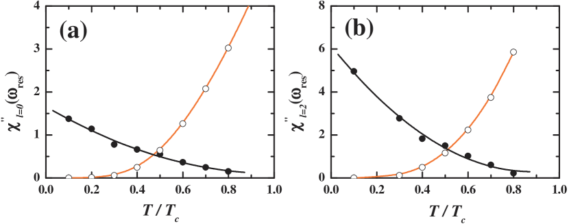
Figure 6: Amplitude of the HFB-RPA resonances (in arbitrary units) from Fig. 5 as a function of reduced temperature $T/T_{c}$ for the monopole (a) and the quadrupole (b). The solid and empty circles refer to the condensate and to the non-condensate, respectively. The lines are guides to the eye.

We present in this section the numerical results of the HFB-RPA for the monopole and quadrupole modes and compare them with those given by the SOBP-RPA and by the HF-RPA. These various theories give somewhat different results for the spectra at intermediate values of the temperature, in the range $0.4T_{c}\leq T\leq 0.8T_{c}$.

In Fig. 5 we plot the HFB-RPA spectral functions at various temperatures. For $k_{B}T\gtrsim\mu$ two main resonances are seen in each spectrum, which can be interpreted as representing the collective oscillations of the non-condensate and of the condensate. The oscillator strength of each resonance has been extracted from the spectra and is shown in Fig. 6 as a function of temperature. Naturally, with increasing $T/T_{c}$ the amplitude of the non-condensate resonances grows (empty circles) while that of the condensate resonances decreases (solid circles). The amplitudes of the modes in the two components of the gas are comparable with each other near $T/T_{c}=0.5$, where the non-condensate fraction is populated by about $30\%$ for our choice of parameters. Above this temperature the strength of the non-condensate resonances increases very rapidly.

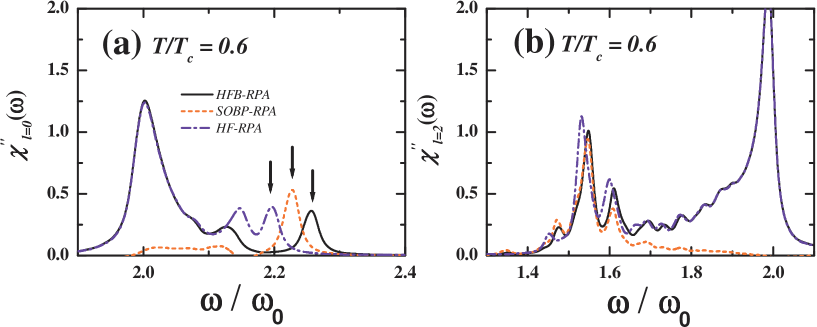
Figure 7: Spectral response (in arbitrary units) as a function of frequency $\omega$ (in units of $\omega_{0}$) for the monopole mode (a) and the quadrupole mode (b), at $T/T_{c}=0.6$ with $\eta=0.01\omega_{0}$ from the HFB-RPA (solid lines), the SOBP-RPA (dashed lines) and the HF-RPA (dot-dashed lines). The arrows in panel (a) point to the condensate resonance position given by each RPA theory. The SOBP-RPA spectra as defined in Eqs. (17) and (18) do not include the contribution from the direct excitation of the non-condensate.

In Fig. 7 we compare with each other the numerical results from the RPA theories for the monopolar and quadrupolar spectra at $T/T_{c}=0.6$. We see that the HF-RPA and HFB-RPA closely agree in their predictions on the main non-condensate resonances for both types of excitations. We also see that all three theories predict essentially very similar results for the main quadrupolar resonance of the condensate, the position of the main peak at $\omega\simeq 1.55\omega_{0}$ in Fig. 7(b) being also in agreement with the result of the HFB-Popov approximation (not shown). In the following we concentrate on the main condensate resonance in the monopolar mode, for which the three theories give rather different predictions as is emphasized by the three arrows in Fig. 7(a). In fact, the partial spectra of condensate and non-condensate show an appreciable overlap in this frequency range, implying a stronger dynamical coupling between the breathing excitations of the two components of the gas and therefore an enhanced sensitivity to the approximations made in the theory.

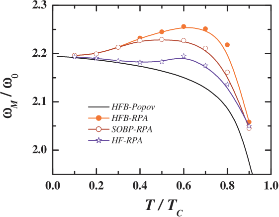
Figure 8: Monopole excitation frequency $\omega_{M}$ (in units of $\omega_{0}$) as a function of reduced temperature $T/T_{c}$, as predicted by various theories: the HFB-Popov (solid line), the HFB-RPA (solid circles), the SOBP-RPA (empty circles) and the HF-RPA (stars). The lines connecting the symbols are guides to the eye.

To better illustrate the difference among the various theories, we extract the monopolar mode frequency of the condensate from the peak in $\chi^{{}^{\prime\prime}}\left(\omega\right)$ and plot it in Fig. 8 as a function of reduced temperature. For comparison we also show the mode frequency given by the HFB-Popov theory (see Sec. II). The most remarkable feature of Fig. 8 is that all three RPA theories show a non-monotonic behavior of the resonance as a function of temperature, in contrast with the prediction of the HFB-Popov theory in which the resonance frequency decreases monotonically with increasing temperature. This difference is due to the dynamical coupling between the condensate and the non-condensate, which is neglected in the mean-field theory and becomes important as the non-condensate is significantly populated.

Let us now compare the three RPA theories, which transcend the mean-field level. At low temperature ($T/T_{c}<0.4$) we observe two different trends: the mode frequencies obtained from the HFB-RPA and from the SOBP-RPA are in close agreement and move upwards with temperature, whereas the mode frequency predicted by the HF-RPA tends to decrease. The latter trend is in good agreement with the HFB-Popov theory, in accord with the proof already given in Ref. mt . The upward trend of the mode frequency with temperature is manifested in all RPA theories at intermediate temperatures, reaching near $T/T_{c}=0.7$ the highest sensitivity to the detailed description of the physical process in which the thermal cloud is driven by its self-generated dynamical potential. Finally, in proximity of the critical temperature all three theories tend to agree as the anomalous density fluctuations disappear.

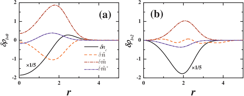
Figure 9: Density fluctuations (in arbitrary units) as functions of the radial coordinate $r$ (in units of $a_{ho}$) for the monopole mode (a) and the quadrupole mode (b), as calculated from the HFB-RPA for $T/T_{c}=0.6$ at the appropriate excitation frequency of the condensate. In both panels the condensate density fluctuation is reduced by a factor of 5 for clarity.

The fact that a large upward frequency shift is found with increasing temperature in both the SOBP-RPA and the HFB-RPA suggests that a significant role is played by the anomalous density fluctuations. In Fig. 9 we show the partial density fluctuations which accompany the monopolar and quadrupolar condensate resonances at $T/T_{c}=0.6$, as calculated from the HFB-RPA. In both modes we find that the anomalous density fluctuations are at this temperature at least comparable in magnitude to the fluctuations of the normal density.

VII Conclusions

In conclusion, we have developed a random-phase theory for the dynamics of a weakly interacting Bose gas under external confinement at finite temperature. In the theory the dynamics of the condensate and of the thermal cloud are treated on the same footing and a previous Hartree-Fock random-phase scheme is extended through the inclusion of the anomalous density fluctuations. The theory satisfies with good numerical accuracy the generalized Kohn theorem and correctly reduces to the second-order Beliaev-Popov theory if one neglects the process in which the thermal cloud is driven by its self-generated potential. It thereby fully includes the Landau-Beliaev damping mechanism.

We have compared the theory with the second-order Beliaev-Popov theory and with the Hartree-Fock random-phase theory by numerical illustrations for a condensate of ⁸⁷Rb atoms inside a spherical trap. The location of the main monopolar and quadrupolar resonances of the thermal cloud are well reproduced in the Hartree-Fock RPA and the frequency of the quadrupole mode of the condensate does not differ significantly from the mean-field HFB-Popov prediction. We have instead found that for $T>0.4T_{c}$ the temperature dependence of the breathing mode frequency of the condensate obtained from the various RPA theories is very different from the HFB-Popov result. A significant role appears to be played in the dynamics of the Bose-condensed gas by the anomalous density fluctuations of the thermal cloud at intermediate temperatures, even though they are known not to affect significantly the thermodynamics of the trapped gas minguzzi97 ; giorgini97 ; guilleumas .

Our results, though restricted to isotropic confinement, may be relevant in connection with the JILA experiments jin97 , where the breathing mode in an anisotropic trap showed a frequency upshift with temperature which could not be accounted for by the HFB-Popov theory burnett . A quantitative comparison between experimental data and the RPA predictions for an anisotropic trap would be interesting for a full test of the theory and we hope to address this issue in future work.

Appendix A The two-particle response functions

We present here a brief explanation on how to derive the response functions used in Eqs. (9) and (10) and list the two-particle response functions of the non-condensate.

Let us consider for example the expression of $\chi_{cc}\left(\mathbf{r},\mathbf{r}^{\prime};\omega\right)$. The most convenient way to obtain it is to calculate the bosonic Matsubara Green’s function with imaginary time variable fetter ,

$$\chi_{cc}\left(\mathbf{r},\mathbf{r}^{\prime};\tau\right)=-\left\langle\text{T}_{\tau}\tilde{\psi}(\mathbf{r},\tau)\tilde{\psi}(\mathbf{r}^{\prime},0)\right\rangle_{0}.$$ (27)

Here T_τ denote the ordering in imaginary time and $\left\langle...\right\rangle_{0}$ denotes the equilibrium statistical average. By expressing the operator $\tilde{\psi}(\mathbf{r},\tau)$ in terms of the Bogoliubov quasiparticle operators $\hat{\alpha}_{i}$ and $\hat{\alpha}_{i}^{+}$, $\tilde{\psi}(\mathbf{r},\tau)=\sum_{j}\left[u_{j}(\mathbf{r})\hat{\alpha}_{j}e^{-\epsilon_{j}\tau}+v_{j}^{*}(\mathbf{r})\hat{\alpha}_{j}^{+}e^{\epsilon_{j}\tau}\right]$, we can rewrite $\chi_{cc}\left(\mathbf{r},\mathbf{r}^{\prime};\tau\right)$ in the form

$$\chi_{cc}\left(\mathbf{r},\mathbf{r}^{\prime};\tau\geq 0\right) = -\left\langle\tilde{\psi}(\mathbf{r},\tau)\tilde{\psi}^{+}(\mathbf{r}^{\prime},0)\right\rangle_{0},$$ (28)

$$= -\sum_{j,k}\left\langle\left[u_{j}(\mathbf{r})\hat{\alpha}_{j}e^{-\epsilon_{j}\tau}+v_{j}^{*}(\mathbf{r})\hat{\alpha}_{j}^{+}e^{\epsilon_{j}\tau}\right]\left[u_{k}(\mathbf{r}^{\prime})\hat{\alpha}_{k}+v_{k}^{*}(\mathbf{r}^{\prime})\hat{\alpha}_{k}^{+}\right]\right\rangle_{0},$$

$$= -\sum_{j}\left[u_{j}(\mathbf{r})v_{j}^{*}(\mathbf{r}^{\prime})\left(1+f_{j}\right)e^{-\epsilon_{j}\tau}+v_{j}^{*}(\mathbf{r})u_{j}(\mathbf{r}^{\prime})f_{j}e^{\epsilon_{j}\tau}\right].$$

We then carry out a Fourier transform with respect to the imaginary time variable $\tau$,

$$\chi_{cc}\left(\mathbf{r},\mathbf{r}^{\prime};i\omega_{n}\right) = \int\limits_{0}^{\beta}d\tau e^{i\omega_{n}\tau}\chi_{cc}\left(\mathbf{r},\mathbf{r}^{\prime};\tau\geq 0\right),$$ (29)

$$= \sum_{j}\left(\frac{u_{j}\left(\mathbf{r}\right)v_{j}^{*}\left(\mathbf{r}^{\prime}\right)}{i\omega_{n}-\epsilon_{j}}-\frac{v_{j}^{*}\left(\mathbf{r}\right)u_{j}\left(\mathbf{r}^{\prime}\right)}{i\omega_{n}+\epsilon_{j}}\right)$$

where $i\omega_{n}=2n\pi i/\beta$. With the analytic continuation $i\omega_{n}\rightarrow\omega+i\eta$ we obtain the expression for $\chi_{cc}\left(\mathbf{r},\mathbf{r}^{\prime};\omega\right)$ in Eq. (11).

The two-particle response functions of the non-condensate can be derived in a similar way. They take the following forms:

$$\chi_{\tilde{n}\tilde{n}}\left(\mathbf{r},\mathbf{r}^{\prime};\omega\right)=\chi_{\tilde{n}\tilde{n}}^{(1)}\left(\mathbf{r},\mathbf{r}^{\prime};\omega\right)+\chi_{\tilde{n}\tilde{n}}^{(2)}\left(\mathbf{r},\mathbf{r}^{\prime};\omega\right)$$ (30)

with

$$\chi_{\tilde{n}\tilde{n}}^{(1)}\left(\mathbf{r},\mathbf{r}^{\prime};\omega\right)=\sum\limits_{ij}\frac{\left(u_{i}^{*}u_{j}+v_{i}^{*}v_{j}\right)\left(u_{i}u_{j}^{*}+v_{i}v_{j}^{*}\right)\left(f_{i}-f_{j}\right)}{\hbar\omega^{+}+\left(\epsilon_{i}-\epsilon_{j}\right)}$$

and

$$\chi_{\tilde{n}\tilde{n}}^{(2)}\left(\mathbf{r},\mathbf{r}^{\prime};\omega\right) = \frac{1}{2}\sum\limits_{ij}\left[\frac{\left(u_{i}v_{j}+v_{i}u_{j}\right)\left(u_{i}^{*}v_{j}^{*}+v_{i}^{*}u_{j}^{*}\right)\left(1+f_{i}+f_{j}\right)}{\hbar\omega^{+}-\left(\epsilon_{i}+\epsilon_{j}\right)}\right.$$

$$\left.-\frac{\left(u_{i}^{*}v_{j}^{*}+v_{i}^{*}u_{j}^{*}\right)\left(u_{i}v_{j}+v_{i}u_{j}\right)\left(1+f_{i}+f_{j}\right)}{\hbar\omega^{+}+\left(\epsilon_{i}+\epsilon_{j}\right)}\right];$$

$$\chi_{\tilde{n}\tilde{m}}\left(\mathbf{r},\mathbf{r}^{\prime};\omega\right)=\chi_{\tilde{m}^{+}\tilde{n}}^{*}\left(\mathbf{r}^{\prime},\mathbf{r};\omega\right)=\chi_{\tilde{n}\tilde{m}}^{(1)}\left(\mathbf{r},\mathbf{r}^{\prime};\omega\right)+\chi_{\tilde{n}\tilde{m}}^{(2)}\left(\mathbf{r},\mathbf{r}^{\prime};\omega\right)$$ (31)

with

$$\chi_{\tilde{n}\tilde{m}}^{(1)}\left(\mathbf{r},\mathbf{r}^{\prime};\omega\right)=2\sum\limits_{ij}\frac{\left(u_{i}^{*}u_{j}+v_{i}^{*}v_{j}\right)u_{i}v_{j}^{*}\left(f_{i}-f_{j}\right)}{\hbar\omega^{+}+\left(\epsilon_{i}-\epsilon_{j}\right)}$$

and

$$\chi_{\tilde{n}\tilde{m}}^{(2)}\left(\mathbf{r},\mathbf{r}^{\prime};\omega\right)=2\sum\limits_{ij}\left[\frac{v_{i}u_{j}v_{i}^{*}v_{j}^{*}\left(1+f_{i}+f_{j}\right)}{\hbar\omega^{+}-\left(\epsilon_{i}+\epsilon_{j}\right)}-\frac{u_{i}^{*}v_{j}^{*}u_{i}u_{j}\left(1+f_{i}+f_{j}\right)}{\hbar\omega^{+}+\left(\epsilon_{i}+\epsilon_{j}\right)}\right];$$

$$\chi_{\tilde{n}\tilde{m}^{+}}\left(\mathbf{r},\mathbf{r}^{\prime};\omega\right)=\chi_{\tilde{m}\tilde{n}}^{*}\left(\mathbf{r}^{\prime},\mathbf{r};\omega\right)=\chi_{\tilde{n}\tilde{m}^{+}}^{(1)}\left(\mathbf{r},\mathbf{r}^{\prime};\omega\right)+\chi_{\tilde{n}\tilde{m}^{+}}^{(2)}\left(\mathbf{r},\mathbf{r}^{\prime};\omega\right)$$ (32)

with

$$\chi_{\tilde{n}\tilde{m}^{+}}^{(1)}\left(\mathbf{r},\mathbf{r}^{\prime};\omega\right)=2\sum\limits_{ij}\frac{\left(u_{i}^{*}u_{j}+v_{i}^{*}v_{j}\right)v_{i}u_{j}^{*}\left(f_{i}-f_{j}\right)}{\hbar\omega^{+}+\left(\epsilon_{i}-\epsilon_{j}\right)}$$

and

$$\chi_{\tilde{n}\tilde{m}^{+}}^{(2)}\left(\mathbf{r},\mathbf{r}^{\prime};\omega\right)=2\sum\limits_{ij}\left[\frac{v_{i}u_{j}u_{i}^{*}u_{j}^{*}\left(1+f_{i}+f_{j}\right)}{\hbar\omega^{+}-\left(\epsilon_{i}+\epsilon_{j}\right)}-\frac{u_{i}^{*}v_{j}^{*}v_{i}v_{j}\left(1+f_{i}+f_{j}\right)}{\hbar\omega^{+}+\left(\epsilon_{i}+\epsilon_{j}\right)}\right];$$

$$\chi_{\tilde{m}\tilde{m}}\left(\mathbf{r},\mathbf{r}^{\prime};\omega\right)=\chi_{\tilde{m}^{+}\tilde{m}^{+}}^{*}\left(\mathbf{r}^{\prime},\mathbf{r};\omega\right)=\chi_{\tilde{m}\tilde{m}}^{(1)}\left(\mathbf{r},\mathbf{r}^{\prime};\omega\right)+\chi_{\tilde{m}\tilde{m}}^{(2)}\left(\mathbf{r},\mathbf{r}^{\prime};\omega\right)$$ (33)

with

$$\chi_{\tilde{m}\tilde{m}}^{(1)}\left(\mathbf{r},\mathbf{r}^{\prime};\omega\right)=4\sum\limits_{ij}\frac{v_{i}^{*}u_{j}u_{i}v_{j}^{*}\left(f_{i}-f_{j}\right)}{\hbar\omega^{+}+\left(\epsilon_{i}-\epsilon_{j}\right)}$$

and

$$\chi_{\tilde{m}\tilde{m}}^{(2)}\left(\mathbf{r},\mathbf{r}^{\prime};\omega\right)=2\sum\limits_{ij}\left[\frac{u_{i}u_{j}v_{i}^{*}v_{j}^{*}\left(1+f_{i}+f_{j}\right)}{\hbar\omega^{+}-\left(\epsilon_{i}+\epsilon_{j}\right)}-\frac{v_{i}^{*}v_{j}^{*}u_{i}u_{j}\left(1+f_{i}+f_{j}\right)}{\hbar\omega^{+}+\left(\epsilon_{i}+\epsilon_{j}\right)}\right];$$

$$\chi_{\tilde{m}\tilde{m}^{+}}\left(\mathbf{r},\mathbf{r}^{\prime};\omega\right)=\chi_{\tilde{m}\tilde{m}^{+}}^{(1)}\left(\mathbf{r},\mathbf{r}^{\prime};\omega\right)+\chi_{\tilde{m}\tilde{m}^{+}}^{(2)}\left(\mathbf{r},\mathbf{r}^{\prime};\omega\right)$$ (34)

with

$$\chi_{\tilde{m}\tilde{m}^{+}}^{(1)}\left(\mathbf{r},\mathbf{r}^{\prime};\omega\right)=4\sum\limits_{ij}\frac{v_{i}^{*}u_{j}v_{i}u_{j}^{*}\left(f_{i}-f_{j}\right)}{\hbar\omega^{+}+\left(\epsilon_{i}-\epsilon_{j}\right)}$$

and

$$\chi_{\tilde{m}\tilde{m}^{+}}^{(2)}\left(\mathbf{r},\mathbf{r}^{\prime};\omega\right)=2\sum\limits_{ij}\left[\frac{u_{i}u_{j}u_{i}^{*}u_{j}^{*}\left(1+f_{i}+f_{j}\right)}{\hbar\omega^{+}-\left(\epsilon_{i}+\epsilon_{j}\right)}-\frac{v_{i}^{*}v_{j}^{*}v_{i}v_{j}\left(1+f_{i}+f_{j}\right)}{\hbar\omega^{+}+\left(\epsilon_{i}+\epsilon_{j}\right)}\right];$$

and finally

$$\chi_{\tilde{m}^{+}\tilde{m}}\left(\mathbf{r},\mathbf{r}^{\prime};\omega\right)=\chi_{\tilde{m}^{+}\tilde{m}}^{(1)}\left(\mathbf{r},\mathbf{r}^{\prime};\omega\right)+\chi_{\tilde{m}^{+}\tilde{m}}^{(2)}\left(\mathbf{r},\mathbf{r}^{\prime};\omega\right)$$ (35)

with

$$\chi_{\tilde{m}^{+}\tilde{m}}^{(1)}\left(\mathbf{r},\mathbf{r}^{\prime};\omega\right)=4\sum\limits_{ij}\frac{u_{i}^{*}v_{j}u_{i}v_{j}^{*}\left(f_{i}-f_{j}\right)}{\hbar\omega^{+}+\left(\epsilon_{i}-\epsilon_{j}\right)}$$

and

$$\chi_{\tilde{m}^{+}\tilde{m}}^{(2)}\left(\mathbf{r},\mathbf{r}^{\prime};\omega\right)=2\sum\limits_{ij}\left[\frac{v_{i}v_{j}v_{i}^{*}v_{j}^{*}\left(1+f_{i}+f_{j}\right)}{\hbar\omega^{+}-\left(\epsilon_{i}+\epsilon_{j}\right)}-\frac{u_{i}^{*}u_{j}^{*}u_{i}u_{j}\left(1+f_{i}+f_{j}\right)}{\hbar\omega^{+}+\left(\epsilon_{i}+\epsilon_{j}\right)}\right].$$

In above expressions $\omega^{+}=\omega+i0^{+}$ and we have used abbreviations such as $u_{i}^{*}u_{j}u_{i}u_{j}^{*}=u_{i}^{*}(\mathbf{r})u_{j}(\mathbf{r})u_{i}(\mathbf{r}^{\prime})u_{j}^{*}(\mathbf{r}^{\prime})$, which means that in the product of four position-dependent functions the first two depend on $\mathbf{r}$ and the latter two on $\mathbf{r}^{\prime}$. $\chi_{ab}^{(1)}$ and $\chi_{ab}^{(2)}$ in the above expressions correspond to the excitation of single thermal quasiparticles and of pairs of thermal quasiparticles, respectively.

References

• (1) D. S. Jin, J. R. Ensher, M. R. Matthews, C. E. Wieman, and E. A. Cornell, Phys. Rev. Lett. 77, 420 (1996).
• (2) D. S. Jin, M. R. Matthews, J. R. Ensher, C. E. Wieman, and E. A. Cornell, Phys. Rev. Lett. 78, 764 (1997).
• (3) M.-O. Mewes, M. R. Andrews, N. J. van Druten, D. M. Stamper-Kurn, D. S. Durfee, C. G. Townsend, and W. Ketterle, Phys. Rev. Lett. 77, 988 (1996).
• (4) D. M. Stamper-Kurn, H.-J. Miesner, S. Inouye, M. R. Andrews, and W. Ketterle, Phys. Rev. Lett. 81, 500 (1998).
• (5) R. Onofrio, D. S. Durfee, C. Raman, M. Köhl, C. E. Kuklewicz, and W. Ketterle, Phys. Rev. Lett. 84, 810 (2000).
• (6) R. J. Dodd, M. Edwards, C. W. Clark, and K. Burnett, Phys. Rev. A 57, R32 (1998).
• (7) D. A. W. Hutchinson, R. J. Dodd, and K. Burnett, Phys. Rev. Lett. 81, 2198 (1998).
• (8) For an overview see, A. Griffin in Bose-Einstein Condensation in Atomic Gases, Proc. Int. School of Physics ”Enrico Fermi”, edited by M. Inguscio, S. Stringari, and C. E. Wieman (Italian Physical Society, 1999).
• (9) A. Minguzzi and M. P. Tosi, J. Phys.: Condens. Matter 9, 10211 (1997).
• (10) P. O. Fedichev and G. V. Shlyapnikov, Phys. Rev. A 58, 3146 (1998).
• (11) M. J. Bijlsma and H. T. C. Stoof, Phys. Rev. A 60, 3973 (1999).
• (12) E. Zaremba, T. Nikuni, and A. Griffin, J. Low Temp. Phys. 116, 277 (1999).
• (13) J. Reidl, A. Csordás, R. Graham, and P. Szépfalusy, Phys. Rev. A 61, 043606 (2000).
• (14) S. Giorgini, Phys. Rev. A 61, 063615 (2000).
• (15) M. Rusch, S. A. Morgan, D. A. W. Hutchinson, and K. Burnett, Phys. Rev. Lett. 85, 4844 (2000).
• (16) S. A. Morgan, M. Rusch, D. A. W. Hutchinson, and K. Burnett, cond-mat/0305535.
• (17) S. T. Beliaev, Sov. Phys. JETP 7, 289 (1958); 7, 299 (1958).
• (18) H. Shi and A. Griffin, Phys. Rep. 304, 1 (1998).
• (19) A. Griffin, Phys. Rev. B 53, 9341 (1996).
• (20) F. Dalfovo, S. Giorgini, L. P. Pitaevskii, and S. Stringari, Rev. Mod. Phys. 71, 463 (1999).
• (21) X.-J. Liu and H. Hu, Phys. Rev. A 68, 033613 (2003); see also X.-J. Liu et al. (unpublished).
• (22) A. L. Fetter and J. D. Walecka, Quantum Theory of Many-Particle Systems (McGraw-Hill, New York, 1971).
• (23) P. Capuzzi and E. S. Hernández, Phys. Rev. A 64, 043607 (2001).
• (24) K. Huang, Statistical Mechanics (Wiley , New York, 1987), pp. 230-238.
• (25) G. Bruun, Y. Castin, R. Dum, and K. Burnett, Eur. Phys. J. D 7, 433 (1999). The divergence is removed by the substitutions $\tilde{m}^{0}\left({\bf r}\right)\rightarrow\tilde{m}^{0}\left({\bf r}\right)-g\Phi_{0}^{2}\left({\bf r}\right)G_{0}^{irr}({\bf r})/2$, $\chi_{\tilde{m}\tilde{m}^{+}}\left({\bf r},{\bf r}^{\prime};\omega\right)\rightarrow\chi_{\tilde{m}\tilde{m}^{+}}\left({\bf r},{\bf r}^{\prime};\omega\right)-\delta({\bf r}-{\bf r}^{\prime})G_{0}^{irr}({\bf r})$, and $\chi_{\tilde{m}^{+}\tilde{m}}\left({\bf r},{\bf r}^{\prime};\omega\right)\rightarrow\chi_{\tilde{m}^{+}\tilde{m}}\left({\bf r},{\bf r}^{\prime};\omega\right)-\delta({\bf r}-{\bf r}^{\prime})G_{0}^{irr}({\bf r})$. Here $G_{0}^{irr}({\bf r})$ is the singular part of the ideal-gas single-particle Green’s function $G_{0}({\bf r+x}/2,{\bf r-x}/2;\omega=0)$, that diverges as $1/x$ for $x$ $\rightarrow 0$.
• (26) J. Reidl, G. Bene, R. Graham, and P. Szépfalusy, Phys. Rev. A 63, 043605 (2001).
• (27) A. Minguzzi, Phys. Rev. A 64, 033604 (2001).
• (28) M. Lewenstein and L. You, Phys. Rev. Lett. 77, 3489 (1996).
• (29) A. Minguzzi, S. Conti, and M. P. Tosi, J. Phys.: Condens. Matter 9, L33 (1997).
• (30) S. Giorgini, L. P. Pitaevskii, and S. Stringari, Phys. Rev. Lett. 78, 3987 (1997).
• (31) F. Dalfovo, S. Giorgini, M. Guilleumas, L. P. Pitaevskii, and S. Stringari, Phys. Rev. A 56, 3840 (1997).