Stochastic energy-cascade model for 1+1 dimensional fully developed
turbulence
Jürgen Schmiegela,
Jochen Cleveb,
Hans C. Eggersc
Bruce R. Pearsond, and
Martin GreinereaNetwork for Mathematical Physics and Stochastics,
Aarhus University, DK–8000 Aarhus, Denmark;
email: schmiegl@imf.au.dk
bICTP, Strada Costiera, 11, 34014 Trieste, Italy;
email: cleve@ictp.trieste.it
cDepartment of Physics, University of Stellenbosch,
7600 Stellenbosch, South Africa;
email: eggers@physics.sun.ac.za
dSchool of Mechanical Materials,
Manufacturing Engineering and Management,
University of Nottingham,
Nottingham NG7 2RD, United Kingdom;
email: bruce.pearson@nottingham.ac.uk
eCorporate Technology,
Information&Communications,
Siemens AG, D-81730 München, Germany;
email: martin.greiner@siemens.com
Abstract
Geometrical random multiplicative cascade processes are often used
to model positive-valued multifractal fields such as the energy
dissipation in fully developed turbulence. We propose a dynamical
generalization describing the energy dissipation in terms of a
continuous and homogeneous stochastic field in one space and one
time dimension. In the model, correlations originate in the overlap
of the respective spacetime histories of field amplitudes. The
theoretical two- and three-point correlation functions are found to
be in good agreement with their equal-time counterparts extracted
from wind tunnel turbulent shear flow data.
Whenever strongly anomalous, intermittent fluctuations, long-range
correlations, multi-scale structuring and selfsimilarity go hand in
hand, the label ‘multifractality’ is attached to the underlying
process. While in this Letter we have in mind fully developed
turbulence of fluid mechanics [1], such processes occur in
various other fields such as formation of cloud and rain fields in
geophysics [2], internet traffic of communication network
engineering [3], and stock returns in finance.
[4], to name but a few.
Random multiplicative cascade models (RMCMs) are commonly used to
model and visualize such phenomena since they generally exhibit
multifractality and reproduce the abovementioned properties
[5]. They are usually implemented through a scale-independent
cascade generator which produces a nested hierarchy of scales and
multiplicatively redistributes the local measure.
In fully developed turbulence, RMCMs have often been employed to model
the energy flux through inertial-range scales. Due to their
multiplicative nature, they can easily reproduce multifractal scaling
exponents associated with the energy dissipation [6], the
latter representing the intermittency corrections [1].
Although the link between such models and the Navier-Stokes equation
remains unclear, recent investigations on multiplier distributions
[7, 8] and scale correlations [9] have shown that
RMCMs do appear to contain more truth than might reasonably be expected
from their phenomenological basis.
Nevertheless, these discrete RMCMs are purely geometrical constructs
and incapable of describing causal dynamical effects of the turbulent
energy cascade. A generalization in this direction is clearly
desirable. Hence, in this Letter, we present a dynamical RMCM in
space-time dimensions which respects causality and
homogeneity. It is related to recent, related efforts
[10, 11, 12, 13], but goes beyond them in its dynamical
interpretation. We first show how this model yields multifractal
scaling for arbitrary -point correlation functions, proceeding
thereafter to compare equal-time two- and three-point correlation
functions to their counterparts obtained from wind-tunnel turbulent
shear flow data.
Our dynamical RMCM is constructed by analogy to the geometrical case,
in which the amplitude of the positive-valued energy-dissipation
field, resolved at the dissipation scale , is defined as the
product of independently and identically distributed random weights
,
(1)
where is an element of a nested hierarchy of scales with the “cascade
generation” and the discrete scale step. The integral
length and the dissipation length represent, respectively,
the largest and smallest length scale of the process. The geometrical
RMCM furthermore requires because of
conservation of energy flux.
We generalize (1) by assuming that is again
the multiplicative product of a stochastic field, but that this field
is now defined on continuous spacetime:
(2)
where is the “index function” described below and by assumption
is a
Lévy-stable white-noise field with index
[14]. For , this corresponds to a non-centered
Gaussian white-noise field. From its characteristic function,
with , the parameter
is fixed to in order to
satisfy the requirement .
Causality, i.e. the requirement that depends on
the past but not the future, dictates that the index function
must be zero for . Demanding also spatial
symmetry around , we are led to the form
(3)
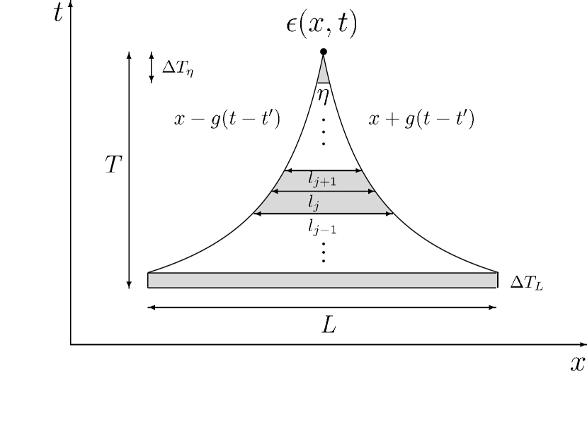
As illustrated in Fig. 1, the causality cone incorporates a
correlation time and a correlation length with . The
exponent of the ansatz (2) can be thought of as a moving
average over the stable white-noise field.
According to (3), the time integration in (2) runs
over . Since to any given time there
corresponds a length scale , there is a joint
hierarchy of length and time scales, so that (2) factorizes
into integrals of over the separate slices shown in Fig. 1,
(4)
In order to interpret as a random multiplicative weight, its
probability density needs to be independent of scale. Since the
are i.i.d., the integration domain of (4)
must therefore be independent of the scale index . Together with
the the boundary conditions and
, this fixes the causality cone to
(5)
for times . To
complete the picture, we need to specify for and . Since on
physical grounds we expect , the simplest choice
is . For the remaining parameter , we
assume ; it will be specified more fully below.
The construction proposed in Eqs. (2)-(5) guarantees
that the one-point statistics of the dynamical RMCM are identical to
its geometrical counterpart. In order to qualify for a complete
dynamical generalization, not only the one-point statistics but the
-point statistics in general should match. Hence, we now consider
the equal-time two-point correlator with and
,
(6)
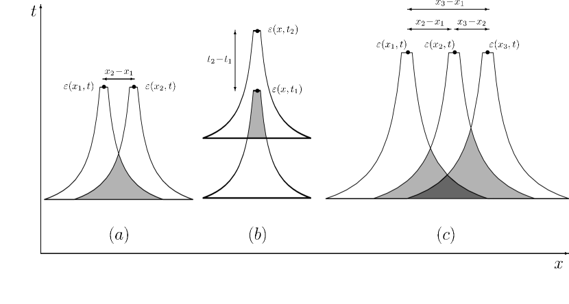
As shown in Fig. 2a, the correlation between two points a distance
apart stems from the overlap region of the
two index functions and . This explains
why, in the second step of (6), can be written solely
in terms of integrals over the overlap region,
(7)
since the contributions from the non-overlapping regions are
statistically independent and hence factorize and cancel. Introducing
the spatio-temporal overlap volume
(8)
and employing basic properties of stable distributions [14],
the expectation of the -th power of is found to be
(9)
Defining the multifractal scaling exponents
, with
,
as well as ,
substitution of (9) into (6) leads to the final
expression for the equal-time two-point correlator:
(10)
Equal-time two-point statistics of our dynamical RMCM in
dimensions hence show multiscaling behavior for
, in complete analogy to the findings of the
corresponding geometrical RMCM [15]. We also note that
setting eliminates the
second factor in (10) leaving to scale rigorously.
Turning to temporal two-point correlations, we follow the same recipe
as for the above. Correlations in this case arise from the overlap
volume illustrated in Fig. 2b, and lead, after an analogous
straightforward calculation, to
(11)
with and . For simplicity, the
parameter has been set to zero. The last step of
(11), valid for and
only, shows that the temporal two-point correlator has
scaling exponents identical to those of the equal-time counterpart.
Although respective spatio-temporal overlap volumes are more
complicated, two-point spacetime correlations with both and can also be derived; see Ref. [16] for a complete analysis. Here, we prefer to continue with
equal-time three-point correlations; their generalization to
equal-time -point correlations is straightforward and explicit
expressions can again be found in Ref. [16]. The corresponding
overlap volumes, illustrated in Fig. 2c, represent the starting point
for a calculation analogous to (7)-(9), which leads
to
(12)
with and for all
. In the case of and small separations
, or for all separations if the parameter
is fine-tuned, this simplifies to
(15)
The comparative ease with which the three-point expressions
(12) and (15) were derived can be traced back to
the fact that the present model incorporates spatio-temporal
homogeneity from the very beginning. This is to be contrasted with the
geometrical RMCMs of (1) which, due to their hierarchical
structure, are not translationally invariant in space. This
non-invariance feeds through to all -point observables and has to
be removed at considerable cost through successive spatial sampling
[17] before the latter can be compared to experimental
counterparts.
While we expect the model proposed in this Letter to find application
in many different phenomena, we demonstrate its qualities through
comparison with fully developed turbulence data. A velocity record of
the longitudinal component, obtained in a wind-tunnel shear flow
experiment [18], was transformed into a one-dimensional
spatial record of the positive-valued surrogate energy dissipation
, where is the
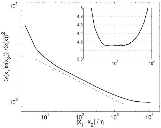
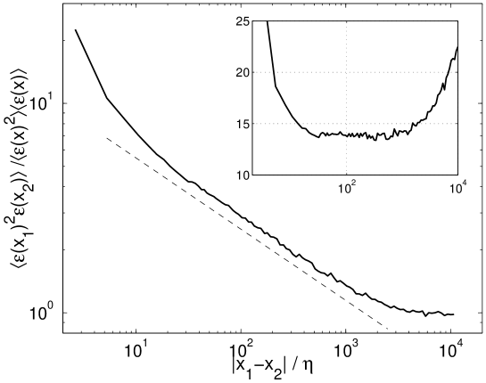
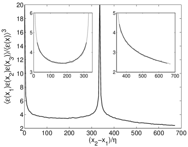
viscosity. The sampled two-point correlations of order and
, are plotted in Fig. 3. Within the inertial range
, the data reveals rigorous power-law
scaling with exponents and . This
fixes the intermittency exponent and the stable index
, which are the relevant model parameters for multifractal
scaling. Once these have been fixed, no further room for adjustment is
left for the theoretical three-point correlation (15),
which is compared to its experimental counterpart in Fig. 4.
Independent of the various combinations for the two-point distances
, the agreement between model and data is
remarkable. This demonstrates that the proposed stochastic process,
whose parameters have been fixed from lowest-order two-point
correlations, is capable to describe the equal-time multivariate
statistics of the turbulent energy dissipation beyond two-point order.
It proofs also that the turbulent energy cascade can be thought of as
a consistent multifractal process.
The dynamical RMCM presented here is a generalization of the
geometrical RMCM. By construction, it is causal, continuous and
homogeneous, does not make use of a discrete hierarchy of scales and
stochastically evolves a positive-valued field in one space and one
time dimension. Several generalizations of this new model come to
mind immediately, such as the stochastic evolution in dimensions
with the optional inclusion of spatial anisotropy, the use of
independently scattered random measures to describe deviation from
log-stability [19], the discretisation of space-time into
smallest cells to model dissipation, and a dynamical RMCM for vector
fields to model the turbulent velocity field.
References
[1]
U. Frisch,
Turbulence,
(Cambridge University Press, Cambridge, 1995).
[2]
D. Schertzer and S. Lovejoy,
J. Geophys. Res. 92 (1987) 9693.
[3]
K. Park and W. Willinger (eds),
Self-similar network traffic and performance evaluation,
John Wiley & Sons, New York, (2000).
[4]
J. Muzy, J. Delour and E. Bacry,
Eur. Phys. J. B 17 (2000) 537.
[5]
J. Feder,
Fractals,
Plenum Press, New York, (1988).
[6]
C. Meneveau and K. Sreenivasan,
J. Fluid Mech. 224 (1991) 429.
[7]
B. Jouault, P. Lipa and M. Greiner,
Phys. Rev. E 59 (1999) 2451.
[8]
B. Jouault, M. Greiner and P. Lipa,
Physica D 136 (2000) 125.
[9]
J. Cleve and M. Greiner,
Phys. Lett. A 273 (2000) 104.
[10]
F.G. Schmitt and D. Marsan,
Eur. Phys. J. B 20 (2001) 3.
[11]
J. Barral and B. Mandelbrot,
Prob. Theory Relat. Fields 124 (2002) 409.
[12]
J.F. Muzy and E. Bacry,
Phys. Rev. E 66 (2002) 056121.
[13]
F.G. Schmitt,
arXiv:cond-mat/0305655.
[14]
G. Samorodnitsky and M. Taqqu,
Stable non-Gaussian random processes,
Chapman & Hall, New York, (1994).
[15]
J. Cleve, K.R. Sreenivasan and M. Greiner,
in preparation.
[16]
J. Schmiegel,
Ein dynamischer Prozess für die statistische Beschreibung
der Energiedissipation in der vollentwickelten Turbulenz,
PhD Thesis, TU Dresden, (2002).
[17]
H.C. Eggers, T. Dziekan and M. Greiner,
Phys. Lett. A 281 (2001) 249.
[18]
B.R. Pearson, P.A. Krogstad and W. van de Water,
Phys. Fluids 14 (2002) 1288.
[19]
O.E. Barndorff-Nielsen and J. Schmiegel,
MAPHYSTO Research Report 2003-20 (http://www.maphysto.dk).
Figure 1:
Causal space-time “cone” for the positive-valued
multifractal field . All field amplitudes
inside the causal space-time “cone” bordered by the
index function (3) contribute multiplicatively to
. See text for further detail.
Figure 2:
Spatio-temporal overlap volumes (shaded) producing the correlation for
the (a) equal-time and (b) temporal two-point correlator, as well as
(c) for the equal-time three-point correlator. To simplify
visualization, parameters have been set to .
Figure 3:
Two-point correlator of orders (a)
and (b) , for the experimental
shear-flow dataset [18] with Taylor Reynolds number
and integral length scale as a function
of the distance in units of the dissipation length .
The insets represent the compensated plots, where the two-point
correlators have been divided by
with and
, respectively.
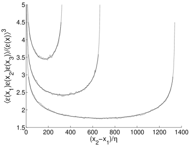
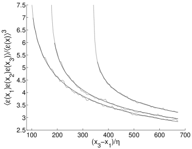
Figure 4:
Comparison between expression (15) and the experimentally
extracted three-point correlator . The same data set as in Fig. 3 has been
used. The scaling exponents and
have already been fixed by the two-point correlators. In part (a), the
experimental three-point correlator is shown for a fixed two-point
distance . The two insets represent the comparison
with (15) for the two regimes and . Part (b) focuses on the regime
with fixed ,
and , respectively, while (c) focuses on the regime
with fixed , and
, respectively. For clarity, from left to right the curves of
(c) have been shifted by , and along the y-axis.