Stochastic Cellular Automata Model for Stock Market Dynamics

Abstract

In the present work we introduce a stochastic cellular automata model in order to simulate the dynamics of the stock market. A direct percolation method is used to create a hierarchy of clusters of active traders on a two dimensional grid. Active traders are characterised by the decision to buy, $\sigma_{i}(t)=+1$, or sell, $\sigma_{i}(t)=-1$, a stock at a certain discrete time step. The remaining cells are inactive, $\sigma_{i}(t)=0$. The trading dynamics is then determined by the stochastic interaction between traders belonging to the same cluster. Extreme, intermittent events, like crashes or bubbles, are triggered by a phase transition in the state of the bigger clusters present on the grid, where almost all the active traders come to share the same spin orientation. Most of the stylized aspects of the financial market time series, including multifractal proprieties, are reproduced by the model. A direct comparison is made with the daily closures of the S&P500 index.

I Introduction

Since the successful application of the Black-Scholes theory for option pricing black73 in 1973 more and more physicists have been attracted by the idea of understanding the behaviour of the market dynamics in terms of complex system theory, where self-organized criticality soc ; bak1997 and stochastic processes mantegna ; paul play important roles. The aim of the microscopic models proposed so far (for general reviews levy2000 ; feigenbaum2003 ) is to reproduce some stylized facts sornette99 concerning the temporal fluctuations of the price indices, $P(t)$. In particular, the logarithmic price returns

$$R(t)=lnP(t+1)-lnP(t),$$ (1)

and the volatility, defined in the present work as

$$v(t)=|R(t)|,$$ (2)

have been studied extensively mantegna from an empirical point of view. The results have shown that while long time correlations are present in the volatility, a phenomenon known as volatility clustering, they cannot be found in the time series of returns. Moreover the latter show an intermittent behaviour that recalls in some aspects hydrodynamic turbulence mantegna97 ; mantegna95 ; frisch , characterized by power law tails in the probability distribution function (pdf). Microsimulations have demonstrated that this kind of behaviour can originate both as a stochastic process with multiplicative noise kaizoji ; krawiecki02 ; takayasu9798 and as a percolation phenomenon stauffer ; stauffer98 ; cont00 .

In order to reproduce these features of real markets we introduce a stochastic cellular automata model, representing an open market. That is, a market where the number of active traders, defined as cells with spin state different from 0, namely $\sigma_{i}(t)=\pm 1$, evolve in time according to a percolation dynamics. The percolation dynamics is chosen in order to simulate the herding behaviour typical of investors sornette03 . According to this, active traders gather in clusters or networks where, following a stochastic exchange of information, they formulate the trading strategy for the next time step. The results obtained by the simulations are then compared with the time series of daily closures of the S&P500 index  mantegna ; plerou99 ; cizeau97 ; gopikrishnan99 ; liu99 ; sornette03 ; ausloos2003 ; Tsallis2003 ; canessa2000 over a period of about 50 years.

Moreover, recently, the fractal properties feder of the price fluctuations have also been investigated for different markets rodrigues01 ; gorski02 ; auloos02 ; dimatteo03 . A common feature found in these studies is the existence of a nonlinear, multifractal spectrum that excludes the possibility of efficient market behaviour bachelier00 . The origin of the multifractality of in the financial time series has also been at the center of discussions lux2001 ; mandelbrot2001 ; lebaron2001 ; stanley2001 . In this paper we consider the multifractal spectrum of the price fluctuations as a stylized fact of the market time series without addressing any question about the underlying process able to generate it. The multifractal spectrum is used as a further test for our model.

A parallel between multifractal and thermodynamical formalism has also been investigated. We found, in agreement with the previous work of Canessa canessa2000 , that the analogue specific heat can provide a good tool to characterize intermittency, that is financial crashes or bubbles, from a thermodynamics-equivalent point of view.

II The Model

In the present work we simulate the financial market dynamics via a stochastic cellular automata model. The agents of the market are represented by cells on a two dimensional grid, 512x128. The $i$th agent at the discrete time step $t$ is characterized by three possible states or spin orientations, $\sigma_{i}(t)=0,\pm 1$. The value $\sigma_{i}(t)=+1$ is associated with the purchase of a stock while $\sigma_{i}(t)=-1$ with selling. The former states are called active. The cells with spin value $\sigma_{i}(t)=0$ are inactive traders. The active traders herd in networks or clusters via a direct percolation method related to a forest fire model stauffer . The information carried by the active traders, that is their spin state, is shared with the other members of the cluster. The percolation dynamics allow a time dependent herding behaviour and the market can be interpreted as an open system not bounded by conservation laws. The clustering process will be discussed in detail in the next subsection.

The trading dynamics is instead related to the synchronous update of the spins of the active traders, ruled by a stochastic exchange of information between them, similar to a random Ising model kaizoji ; krawiecki02 . A particular feature of the present simulation is that the information is not spread all over the grid, as in other multi-agent scenarios kaizoji ; krawiecki02 , but it is limited by the clusters of interaction previously defined. The mechanism for the spin dynamics is explained in “stochastic trading dynamics” subsection.

II.1 Percolation Clustering

One of the aims of our cellular automata model is to reproduce the herding behaviour of active traders sornette03 . We refer to herding behaviour as the tendency of people involved in the market to aggregate in networks or clusters of influence. The traders then use the information obtained by their network in order to formulate a market strategy. Even if the topological structure of these networks of information is not important, since several kinds of long range interaction are available nowadays krawiecki02 , the number of connections for each trader must be, in any case, finite and not extended over the whole market. In this framework a direct percolation method is used to simulate herding dynamics between active traders. If we assume that the neighbours of influence are those of von Neumann (up, down , left, right), the percolation is fixed by the following parameters:

$p_{h}$: the probability that an active trader can turn one of his inactive neighbours into an active one at the next time step, $\sigma_{i}(t)=0\rightarrow\sigma_{i}(t+1)=\pm 1$. This simulates the fact that certain information possessed by a trader may induce a potential trader to join the market dynamics.

$p_{d}$: the probability that an active trader diffuses and so becomes inactive, $\sigma_{i}(t)=\pm 1\rightarrow\sigma_{i}(t+1)=0$, due to each of his inactive neighbour. This mimics the fact that only traders at the borders of a network, that is the weaker links, can quit the market.

$p_{e}$: the probability that a non trading cell spontaneously decides to enter the market dynamics, $\sigma_{i}(t)=0\rightarrow\sigma_{i}(t+1)=\pm 1$.

The values of the adimensional parameters, $p_{h}$, $p_{d}$ and $p_{e}$, influence the stability of the system and the percentage of active traders on the grid. In order to test different market activities we fix the values $p_{d}=0.05$ and $p_{e}=0.0001$ while we tune the parameter $p_{h}$. At the beginning of the simulation the grid is loaded randomly with a small percentage of active traders and then the system is permitted to evolve according to the previous rules. If we are in a stable range of the parameter $p_{h}$, after a transient period that depends both on the parameter values and the initial number of active cells, the number of active traders on the grid begins to fluctuate around a certain average, as shown in Fig. 1 (Top). The market can be considered open since the number of agents changes dynamically in time. In this regime, the competition between herding and diffusion produces a power law distribution of the cluster size, as shown in Fig. 1 (Bottom), $\rho(S)\approx S^{-\lambda}$, where $S$ is the cluster dimension, defined as the number of active cells belonging to the same cluster, and $\lambda>0$, creating a hierarchy of networks. This hierarchy is necessary if were are to take into account a real aspect of the market, namely that different traders also have different trading powers. A reasonable assumption is that people having a larger number of sources of information, so belonging to greater clusters, can be associated with professional investors that, most likely, are able to move a greater amount of stocks compared to the occasional investor. Using this assumption we are able to define a proper weight for the trading power of different cells, as we will discuss in the next subsection.

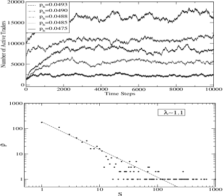
Figure 1: Top: Different values of the parameter H produce different activities of traders on the grid. Bottom: Cluster size distribution for $p_{h}=0.0485$ at $t=9000$.

A similar percolation model has also been used to reproduce some statistical and geometrical features of solar activity wentzel ; vlahos .

II.2 Stochastic Trading Dynamics

The dynamics of the spins of the active traders, $\sigma^{k}_{i}(t)=\pm 1$ for $i=1,...,N^{k}(t)$ (where the superscript $k$, from now on, refers to the $k$th cluster of the grid configuration at time step $t$) follows a stochastic process that mimics the human uncertainty in decision making krawiecki02 . Their values are updated synchronously according to a local probabilistic rule: $\sigma^{k}_{i}(t+1)=+1$ with probability $p^{k}_{i}$ and $\sigma^{k}_{i}(t+1)=-1$ with probability $1-p^{k}_{i}$. The probability $p^{k}_{i}$ is determined, by analogy to heat bath dynamics with formal temperature $k_{b}T=1$, by

$$p^{k}_{i}(t)=\frac{1}{1+e^{-2I^{k}_{i}(t)}},$$ (3)

where the local field, $I^{k}_{i}(t)$, is

$$I^{k}_{i}(t)=\frac{1}{N^{k}(t)}\sum_{j=1}^{N^{k}(t)}A^{k}_{ij}\sigma^{k}_{j}(t)+h^{k}_{i}.$$ (4)

The $A^{k}_{ij}(t)$ are time dependent interaction strengths between agents and $h^{k}_{i}(t)$ is an external field reflecting the effect of the environment krawiecki02 . The interaction strengths and the external field change randomly in time according to $A^{k}_{ij}(t)=A\xi^{k}(t)+a\eta_{ij}(t)$ and $h^{k}_{i}(t)=h\zeta^{k}_{i}(t)$. The variables $\xi^{k}(t),\eta_{ij}(t),\zeta^{k}_{i}(t)$ are random variables uniformly distributed in the interval (-1,1) with no correlation in time or space. The measure of the strengths of the previous terms, $A$, $a$ and $h$, are constant and common for all the grid.

In this contest the dynamics of the price index, $P(t)$, can be easily derived if we assume that the index variation is proportional to the difference between demand and supply,

$$\frac{dP}{dt}\propto xP,$$ (5)

and using a weighted average for the orientation of the spins,

$$x(t)=\beta\sum_{k=1}^{N_{cl}(t)}\sum_{i=1}^{N^{k}(t)}N^{k}(t)\sigma^{k}_{i}(t),$$ (6)

where $N_{cl}(t)$ and $N^{k}(t)$ are, respectively, the number of clusters on the grid and the size of the $k$th cluster, while $\beta$ is a normalization constant. The relation (6) follows from the assumption of proportionality between the financial power of an active cell and the size of the cluster to which it belongs. A justification of this relation is that professional investors, able to move larger amounts of capital, are more likely to be linked with a large number of other investors than the occasional traders. From (5) we find that the logarithm of the price returns (1), that is the fundamental quantity we aim to model, is proportional to the average orientation defined in (6), $R(t)\propto x(t)$.

III Numerical Results

We compare the results of our model with the Standard & Poor 500 (S&P500) index that is one of the most widely used benchmarks for US equity performance. The database analyzed is composed by of the daily indices from 3/1/1950 to 18/7/2003 for a total of 13468 data. The time series of the index prices, $P(t)$, is converted into the logarithmic returns (1) and then normalized over the time interval, $T$,

$$r(t)=\frac{R(t)-\langle R(t)\rangle_{T}}{\sigma(R(t))}.$$ (7)

where $\langle\ldots\rangle_{T}$ denotes the temporal average and $\sigma$ is the standard deviation. In this way all the sets of returns will have zero average and $\sigma=1$.

Before discussing the results we briefly describe the behaviour of the cellular automata with respect to changes of the parameters. Regarding the percolation, the herding parameter $p_{h}$, as previously seen, determines the concentration of active traders on the grid. For a low concentration the active traders will be distributed in small clusters and the information will be extremely split up on the grid. In this case large coherent events will be more rare. A higher concentration, where clusters of the order of a thousand cells are present, allows large events to occur with higher frequency. In fact, the phase transition of large clusters can easily trigger a crash or a bubble in the market. Time series related to a higher herding parameter are therefore more intermittent. We can then infer that a market made by small groups of traders behaves like a noisy market, while big crashes or bubbles must necessarily be related to the interaction of large networks and so to a kind of crowd behaviour. For most of the simulations we fixed the parameter $p_{h}=0.0493$ in order to have bigger clusters, with $S^{max}(t)$ of the order of 2500 cells.

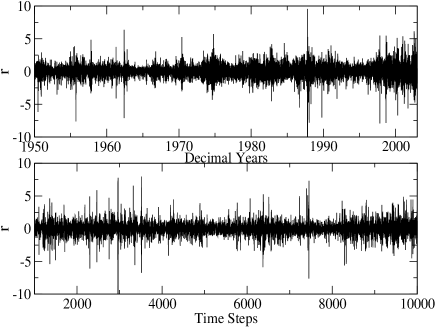
Figure 2: Top: Normalized logarithmic returns for the S&P500. Bottom: Time series of returns reproduced with the simulation with $p_{h}=0.0493$, $A=1.8$ and $h=0$.

The strength $A$ also plays an important role in the trading dynamics. With $p_{h}$ fixed, this parameter is related to the intermittency of the system. Both for large values of the activity ($A>10$) and for $A\rightarrow 0$ we observe an approach of the pdf toward a Gaussian-like shape. That is very, large fluctuations become more and more rare, and $A$ can be regarded as a temporal scale for the system, similar to the activity parameter in the Cont-Bouchaud model cont00 . In spite of this some large fluctuations can be still identified. This is probably one of the main differences between the Cont-Bouchaud model and the present. In fact Monte Carlo simulations of the former stauffer98 show that an increase of the activity brings a rapid convergence toward a Gaussian distribution because a large number of clusters are trading at the same time following a random procedure of decision making cont00 ; stauffer98 : there are no clusters that can influence the market more than others and so the resulting global interaction is noise-like. In our model fluctuations are always allowed because of the heat bath dynamics. Clusters of active traders can always be subjected to phase transitions, independently of the state of other clusters, creating a displacement between demand and supply.

In order to reproduce the behaviour of financial time series we work with $1.5<A<2.5$. In this range there is a nonlinear dependence of the intermittency on $A$. The value of the parameter $a$ is fixed by the relation $a=2A$, already used in the work of Krawiecki et al. krawiecki02 . However, we note that the ratio $a/A$ is actually not essential in reproducing the intermittency found in real data. Even the parameter $h$ does not have a central role in the simulation, as long as $h<<1$. In fact, the percolation dynamics of the active traders already introduces a natural noise. In most of the runs we simply set $h=0$.

Now we discuss the results of the cellular automata. In Fig. 2 (Top) and Fig. 2 (Bottom) the normalized logarithmic returns of the S&P500 and of the simulation are shown, respectively. The average number of active traders, in the stable regime, is $\approx 16000$, as shown in Fig. 1 (Top). The model reproduces the intermittent behaviour of the S&P500 time series, as expressed by the leptokurtic pdf of Fig.3. The tails of the distribution follow a power law decay, reflecting the fact that large coherent events, far from the average, are likely to occur with a frequency higher than expected for a random process (where the shape would be a Gaussian). These large events are related to financial crashes or bubbles of the market and, in our model, to a phase transition in the spin state of large networks of active traders, as we will discuss further on. From a power law fit, $\rho(r)\approx r^{-1-\gamma}$ (for $|r|>2$), we find $\gamma\approx 3$ for both the S&P500 and the model, confirming the good agreement between the two.

The problem of finding the best distribution describing the price returns is a very important issue from a practical point of view mantegna . The standard Black-Scholes theory for option pricing black73 ; mantegna ; paul assumes that the returns are normally distributed. This fact has been proven to be empirically false, as shown also in Fig. 3 (see Ref. mantegna for a general reference). Finding a more appropriate distribution would be an important improvement in this field of research.

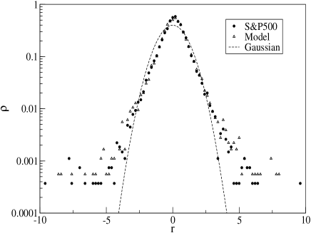
Figure 3: Probability distribution function for the S&P500 computed with daily data from 31/1/1950 to 18/7/2003 and the model. A Gaussian is also plotted for comparison. The parameters used are $p_{h}=0.0493$, $A=1.8$ and $h=0$.

In order to understand the trading dynamics of the automata we also show two snapshots of the grid configuration, the first during a normal session, Fig.4 (Top), and the second during a crash, Fig.4 (Bottom). During the normal session the orientations of the spins are distributed uniformly over the various clusters and there is no sharp difference between demand and supply. The situation is different during a crash. In this case the clusters at the top of the hierarchy, the bigger ones, play a fundamental role. In fact they undergo a phase transition where the greatest part of their spins share the same orientation. The capacity of the clusters to generate a coherent orientation of the spins, and hence of their trading state, can be interpreted in terms of a multiplicative noise process paul ; liu99 , where the collective synchronization arises as a result of the randomly varying interaction strengths between agents. The peculiarity of our model is that crashes or bubbles (sudden price changes) are related not to a phase transition of the whole market krawiecki02 ; kaizoji but rather to a phase transition in one or more of the larger clusters that have a greater influence on the trading session. This behaviour is probably closer to the real market where the synchronization of trading opinion is more likely to happen between large groups of traders than over the whole market.

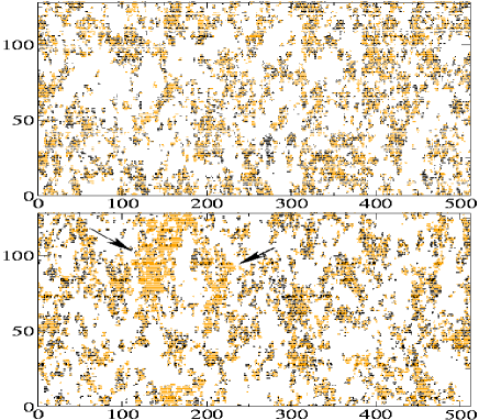
Figure 4: Top: snapshot of the grid during a normal trading period. The black cells are the buyers while the orange ones are the sellers. The parameters used in this simulation are $p_{h}=0.0493$, $A=1.8$ and $h=0$. Bottom: the same simulation during a crash. Large clusters of sellers are indicated by arrows.

The temporal correlations of the logarithmic returns and of the volatility are investigated via the autocorrelation function, defined as

$$c(\tau)=\sum_{t=1}^{T-\tau}x(t+\tau)x(t),$$ (8)

where T is the length of the time series and $\tau$ is a time delay for the normalized variable $x(t)$. The results for both the model and the S&P500 are shown in Fig.5 (Top) and Fig.5 (Bottom), respectively. While the temporal correlation for the returns is lost almost immediately, the volatility manifests a slow decay in time, related to the phenomenon of volatility clustering. The previous temporal dependencies have been found in both real data and in the simulation.

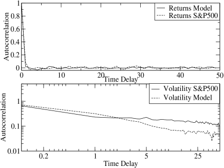
Figure 5: Top: Autocorrelation function for the price returns. Bottom: Autocorrelation function for the volatilities. In both the graphs the parameters used for the model are $p_{h}=0.0493$, $A=1.8$ and $h=0$.

IV Multifractal Analysis

It is also worth pointing out that financial time series present an inherent multifractality feder . In the past few years the work of many authors rodrigues01 ; gorski02 ; auloos02 ; dimatteo03 has been addressed to the characterization of the multifractal properties of financial time series, and nowadays multifractality can be considered as a stylized fact. In order to study the multifractal properties of our model we use the generalized Hurst exponent mandelbrot , $H(q)$, derived via the $q-$order structure function,

$$S_{q}(\tau)=\langle|x(t+\tau)-x(t)|^{q}{\rangle_{T}}\propto\tau^{qH(q)},$$ (9)

where $x(t)$ is a stochastic variable over a time interval $T$ and $\tau$ the time delay. The generalized Hurst exponent, defined in (9), is an extension of the Hurst exponent, $H$, introduced in the context of reservoir control on the Nile river dam project, around 1907 feder ; hurst51 . This technique provides a sensitive method for revealing long-term correlations in random processes. If $H(q)=H$ for every $q$ the process is said to be monofractal and $H$ is equivalent to the original definition of the Hurst exponent. This is the case of simple Brownian motion or fractional Brownian motion.

If the spectrum of $H(q)$ is not constant with $q$ the process is said to be multifractal. From the definition (9) it is easy to see that the function $H(1)$ is related to the scaling properties of the volatility. By analogy with the classical Hurst analysis, a phenomenon is said to be persistent if $H(1)>1/2$ and antipersistent if $H(1)<1/2$. For uncorrelated increments, as in Brownian motion, $H(1)=1/2$. In Fig. 6 a comparison is shown between the multifractal spectra of the model and the S&P500 obtained from the prices time series. It is clear that both processes have a multifractal structure and the price fluctuations cannot be associated with a simple random walk as in the classical efficient market hypothesis bachelier00 .

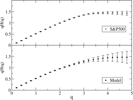
Figure 6: Multifractal spectra for the S&P500 in the period 31/1/1950 to 18/7/2003 (top) and the model (bottom). For the latter $p_{h}=0.0493$, $A=1.8$ and $h=0$.

The multifractality of the time series can also be discussed in terms of thermodynamic equivalents, according to multifractal physics lee88 ; canessa1993 ; vollhardt97 ; canessa2000 . In this approach we divide the time series, $x(t)$ , for $t=1,...,L$ into $\mathcal{N}$ equal sub-intervals. Then we can write the following measure for each of these,

$$\mu_{i}(\tau)=\frac{|x(t+\tau)-x(t)|}{\sum_{t=1}^{\mathcal{N}}|x(t+\tau)-x(t)|},$$ (10)

with $i=1,...,\mathcal{N}$ and $\tau$ the time delay. The quantity $\mu_{i}(\tau)$ can be viewed as a normalized probability measure. The corresponding generating function is given by

$$Z(q,\mathcal{N})=\sum_{i=1}^{\mathcal{N}}\mu_{i}(\tau)^{q}\propto\mathcal{N}^{-\chi_{q}},$$ (11)

that is an analogue of the partition function in thermodynamics. According to Ref. lee88 the scaling exponent $\chi_{q}$ is directly related to the generalized multifractal dimension $D_{q}$ feder ,

$$\chi_{q}\equiv(q-1)D_{q}.$$ (12)

If we consider $\chi_{q}$ as the free energy of our system, Eq.(12) provides a link between the classical thermodynamical formalism and multifractality. Assuming $q$ as an equivalent temperature, we can define an analogue specific heat lee88 ; canessa1993 ; canessa2000 ; ivanova02 ,

$$C_{q}=-\frac{\partial^{2}\chi_{q}}{\partial q^{2}}.$$ (13)

The previous equation for $C_{q}$ can also be written in terms of singular measure formalism davis94 . In this framework we define a measure, $\epsilon(1,t)$, as

$$\epsilon(1,t)=\frac{|x(t+1)-x(t)|}{\frac{1}{L-1}\sum_{t=1}^{L-1}|x(t+1)-x(t)|}.$$ (14)

We can then generate a series of measures on shorter intervals of length $\delta$, $\epsilon(\delta,l)$ where $\delta$ is an integer power of two and $l$ is the index of the first point of the sub segments at that resolution. The average measure in the interval [$l,l+\delta$] is

$$\epsilon(\delta,l)=\frac{1}{\delta}\sum_{l^{\star}=l}^{l+\delta-1}\epsilon(1,l^{\star}),$$ (15)

for $l=0,...,L-\delta$. In this case we have a scaling property for the ensemble average with respect to the scale $\delta$:

$$\langle\epsilon(\delta,l)\rangle\propto\delta^{-K_{q}}.$$ (16)

In a multifractal process the exponent $K_{q}$ is a nonlinear function of $q$ related to the intermittency of the time series and to the generalized dimension via hentschel83 ; halsey86

$$(q-1)D_{q}=q-1-K_{q}.$$ (17)

From (13) and (17) we have that ivanova02 ,

$$C_{q}=\frac{\partial^{2}K_{q}}{\partial q^{2}}.$$ (18)

Following Ref. canessa2000 we have found the analogue specific heat for both the S&P500 and for the price time series generated by our model, see Fig.7. For $\tau=1$ we observe a double-humped shape for both the model and the empirical data. If we take longer time delays the shoulder on the right hand side disappears, leaving only a sharp peak, similar to a first order phase transition around $q=-1.5$. The results are in agreement with the analysis of Canessa canessa2000 and recall the Hubbard model for small to intermediate values of the local interaction vollhardt97 . As also suggested in canessa2000 , the second peak is due to the large fluctuations at small scales, that is crashes and bubbles. Increasing the time delay means that the fluctuations tend to be smoothed and the time series of returns approach a noise-like regime. For this reason the analogue specific heat shapes for $\tau=100$ are basically indistinguishable. From this argument we can interpret the analogue specific heat, and in particular the second peak for low time delays, as a way to characterize crashes, or in general the degree of intermittency in a time series. The difference in the shapes and heights of the shorter peak for $\tau=1$ is due to a slightly different correlation of the fluctuations in the two time series. Moreover, in the model we can link the shorter peak to the physical phase transition in the spin state of a network of traders.

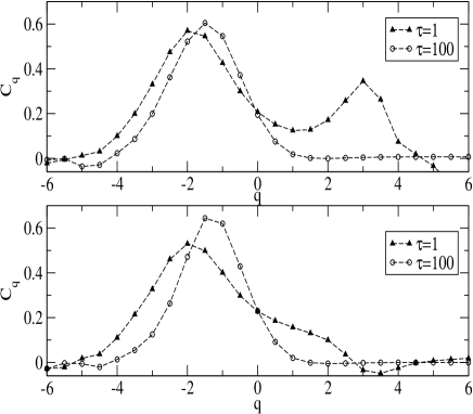
Figure 7: Top: analogue specific heat for the S&P500 from 31/1/1950 to 18/7/2003 for two different time delays, namely $\tau=1$ and $\tau=100$. A sharp peak is clearly visible around $q=-1.5$. The second peak on the right hand side disappears increasing the temporal delay. The $C_{q}$ curves have been computed for the logarithm of the price using the algorithm in davis94 for $K_{q}$. Bottom: analogue specific heat for the model with parameters $p_{h}=0.0493$, $A=1.8$ and $h=0$. The double humped shaped for small temporal delays is visible also here.

V Conclusions

In this paper we have introduced a stochastic cellular automata model for the dynamics of the financial markets. The main difference between our model and other stochastic simulations based on spin orientation of agents krawiecki02 ; kaizoji is the temporal evolution of the networks of interaction and therefore the concept of an “open” market. The active traders follow a direct percolation dynamics in order to aggregate in networks of information. This makes our simulation, even if still a raw approximation, surely closer to the real market, where no conservation rules for the number of agents can be claimed. Crashes and bubbles can be interpreted as a synchronization of the spin orientation of the more influential networks in the market. Moreover, the introduction of a limitation in the number of interacting agents reduces drastically the number of computations on the grid per time step. In a system where all the agents interact with each other this number goes like $N_{a}^{2}$, being $N_{a}$ the number of active agents, while in our model, considering the distribution of the clusters, it is easy to see that it goes like $N_{a}^{2-\lambda}$. The value of $\lambda$ found for several herding parameters, $p_{h}$, is $\lambda\approx 0.6\div 1.4$, so that the computational cost is much lower for the present model. This gives one the possibility to simulate the market using a very large range of agents. The model is able to reproduce most of the stylized aspects of the financial time series, supporting the idea that crashes and bubbles are related to a collective synchronization in the trading behaviour of large networks of traders, where the information is exchanged according stochastic interaction between them.

- (1) F. Black and M. Scholes, J. Political Economy 81, 637 (1973); R.C. Merton, Bell J. Econom. Manage. Sci. 41, 141 (1973).
- (2) P. Bak et al., Phys. Rev. Lett.,59, 381 (1987); P. Bak et al., Phys. Rev. A,38, 364 (1988); P. Bak,How Nature Works,(Springer-Verlag, New-York, 1999); H. J. Jensen, Self-Organized Criticality: Emergent Complex Behavior in Physical and Biological Systems, (Cambridge University Press, Cambridge, 1998).
- (3) P. Bak et al.,Physica A 246, 430 (1997).
- (4) R. N. Mantegna and H. E. Stanley,An Introduction to Econophysics: Correlation and Complexity in Finance,(Cambridge University Press, Cambridge, 1999); J.-P. Bouchard and M. Potters, Theory of Financial Risk, (Cambridge University Press, Cambridge, 1999).
- (5) W. Paul and J. Baschnagel, Stochastic Processes: From Physics to Finance, (Spriger-Verlag, Berlin,1999).
- (6) H. Levy, M. Levy and S. Solomon, Microscopic Simulations of Financial Markets, (Academic Press, New York, 2000).
- (7) J. Feigenbaum, Rep. Prog. Phys. 66, 1611 (2003).
- (8) D. Sornette et al., arXiv:cond-mat/9909439, (1999).
- (9) R. N. Mantegna and H. E. Stanley, Physica A 239, 225 (1997).
- (10) R. N. Mantegna and H. E. Stanley, Nature 376, 46 (1995).
- (11) U. Frisch, Turbulence, (Cambridge University Press, Cambridge, 1995).
- (12) T. Kaizoji, Physica A 287, 493 (2000).
- (13) A. Krawiecki et al., Phys. Rev. Lett.89, 158701 (2002); A. Krawiecki et al., Physica A 317, 597 (2003).
- (14) H. Takayasu et al., Phys. Rev. Lett. 79, 966 (1997); H. Takayasu and M. Takayasu, Physica A 269, 24 (1999).
- (15) D. Stauffer, Introduction to Percolation Theory, (Taylor & Francis, London,1985).
- (16) R. Cont and J.-P. Bouchaud, Macroeconom. Dyn., 4, 170 (2000).
- (17) D. Stauffer and T.J.P. Penna, Physica A 256, 284 (1998).
- (18) J. Feder, Fractals, (Plenum Press, New York & London, 1988).
- (19) C. Rodrigues Neto et al., Physica A 295, 215 (2001).
- (20) A.Z. Gorski et al., Physica A 316, 296 (2002).
- (21) M. Ausloos and K. Ivanova, Comp. Phys. Comm. 147, 582 (2002).
- (22) T. Di Matteo et al., Physica A 324 183 (2003).
- (23) L. Bachelier, Ann.Sci.de L’Ecole Norm.Sup. III, 21 (1900).
- (24) T. Lux, Quantitative Finance 1(6), 632 (2001).
- (25) B.B. Mandelbrot, Quantitative Finance 1(6), 641 (2001).
- (26) B. LeBaron, Quantitative Finance 1(6), 621 (2001).
- (27) E.H. Stanley and V. Plerou, Quantitative Finance 1(6), 563 (2001).
- (28) D. Sornette, Phys. Rep. 378, 1 (2003).
- (29) V. Plerou et al., Phys. Rev. Lett. 83, 1471 (1999).
- (30) P. Cizeau et al., Physica A 245, 441 (1997).
- (31) P. Gopikrishnan et al., Phys. Rev. E 60, 5305 (1999);P. Gopikrishnan et al., Physca A 287, 362 (2000).
- (32) D. G. Wentzel and P.E. Seiden, Astrophys.J. 390, 280 (1992); D. G. Wentzel and P.E. Seiden, Astrophys.J. 460, 522 (1996).
- (33) L. Vlahos et al., Astrophys.J. Lett., 575, L87 (2002); L. Vlahos, Euroconference and IAU Colloquium 188 on “Magnetic Coupling of the Solar Atmosphere”, Santorini, Greece, 2002, download at http://www.astro.auth.gr/.
- (34) Y. Liu et al., Phys. Rev. E 60, 1390 (1999); P. Gopikrishnan et al., Phys. Rev. E 60, 5305 (1999).
- (35) B. Mandelbrot, Fractals and Scaling in Finance, (Springer, New York, 1997).
- (36) H. Hurst, Trans. Amer. Soc. Civil Eng. 116, 770 (1951).
- (37) C. Tsallis, J. Stat. Phys., 52, 479 (1988).
- (38) C. Tsallis, Brazilian Journal of Physics, 29, 1 (1999);
- (39) F. M. Rosa et al., Nonlinea Analysis 47, 3521 (2001); H. Gupta and J. Campanha, Physica A 309, 381 (2002); F. Michael and M.D. Johonson, Physica A 320, 525 (2003).
- (40) M Ausloos. and K. Ivanova, Phys. Rev. E 68, 046122 (2003).
- (41) C. Tsallis et al., Physica A 324, 89 (2003).
- (42) J. Lee and H.E. Stanley, Phys. Rev. Lett. 61, 2945 (1988).
- (43) D. Vollhardt, Phys. Rev. Lett. 78, 1307 (1997).
- (44) E. Canessa, Phys. Rev. E 47, R5 (1993).
- (45) E. Canessa, J. Phys. A: Math. Gen. 33, 3637 (2000).
- (46) K. Ivanova et al., Physica A 308, 518 (2002).
- (47) A. Davis et al., J. Geophys. Res. 99, 8055 (1994).
- (48) H.G.E. Hentschel and I. Procaccia, Physica D 8, 435 (1983).
- (49) T.C. Halsey et al., Phys. Rev. A 33, R1141 (1986)