First-Principles Study of Integer Quantum Hall Transitions in Mesoscopic Samples

Abstract

We perform first principles numerical simulations to investigate resistance fluctuations in mesoscopic samples, near the transition between consecutive Quantum Hall plateaus. We use six-terminal geometry and sample sizes similar to those of real devices. The Hall and longitudinal resistances extracted from the generalized Landauer formula reproduce all the experimental features uncovered recently. We then use a simple generalization of the Landauer-Büttiker model, based on the interplay between tunneling and chiral currents – the co-existing mechanisms for transport – to explain the three distinct types of fluctuations observed, and identify the central region as the critical region.

Although the Integer Quantum Hall Effect (IQHE) is a generally well understood phenomenon, recent experiments on mesoscopic samples Peled1 ; Peled2 uncovered unexpected behavior in the seemingly noisy fluctuations of the Hall ($R_{H}$) and longitudinal ($R_{L}$) resistances. Previously, fluctuations in resistance had been observed in mesoscopic samples with a phase coherence length $L_{\phi}$ larger than the sample size Timp ; Simmons ; Cobden ; they are totally random, similar to universal conductance fluctuations Fisher . By contrast, Peled et. al. find Peled1 ; Peled2 that the transition between the $n^{th}$ and $(n+1)^{st}$ plateaus of the IQHE has three distinct regimes: (i) on the high-$B$ side, both $R_{H}$ and $R_{L}$ have large but correlated fluctuations, such that $R_{L}+R_{H}=h/ne^{2}$; (ii) for intermediate $B$ values, $R_{H}$ and $R_{L}$ continue to exhibit fluctuations, but their sum is no longer constant; and (iii) on the low-$B$ side, $R_{H}=h/(n+1)e^{2}$ has no fluctuations, whereas $R_{L}$ still does. Moreover, $R_{L}+R_{H}=R_{2t}$ holds for all $B$ values Peled2 . Changing the sign of the magnetic field $B\rightarrow-B$ also has interesting consequences, as discussed later. For $n=0$, regions (i) and (ii) are replaced by the transition to the insulating phase Peled1 . In this Letter, we explain the physics behind these observations in a unified theory, and analyze the implications for further experimental and theoretical study.

The relation $R_{L}+R_{H}=R_{2t}$ was first proposed by Streda et. al. MacDonald , while the fluctuations of regime (iii) are reminiscent of Jain and Kivelson’s theory on the resistance fluctuations of narrow samples Jain . These theories were questioned by Büttiker Buttiker1 , based on formulas appropriate for a four-terminal geometry Buttiker2 . We take an approach similar to Büttiker’s and use the multi-probe Landauer formula Buttiker2 ; Baranger to calculate the resistances measured experimentally. However, we mirror the experiments by including six contacts in our model, namely the four voltage probes plus the source and the drain for the electrical current. Our model enables us to calculate both $R_{L}$ and $R_{H}$, and reveals the very rich physics underlying the observation of the mesoscopic IQHE.

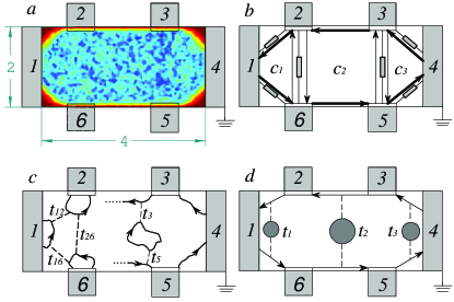
Figure 1: (color online) (a) Typical potential $V_{d}+V_{b}$ of a $4\mu$m$\times 2\mu$m sample. (b) Chiral (arrows) and tunneling (resistors) currents in our model. This direction of chiral currents corresponds to $B$ entering the page. (c) Some semi-classical current distributions parameterized by our model. (d) Jain-Kivelson tunneling for high-$\nu$. See text for further details.

The response function of the system is a $6\times 6$ conductance matrix $\hat{g}$, with which the current-voltage relation reads $I_{\alpha}=\sum_{\beta}g_{\alpha\beta}V_{\beta}$. Here, $I_{\alpha}$ is the out-going current on the contact $\alpha=1,\cdots,6$ and $V_{\alpha}$ is the corresponding voltage. For a mesoscopic Hall bar, $\hat{g}$ characterizes the electrical response (since the system is inhomogeneous, local quantities such as the current density are not conceptually well-defined). $\hat{g}$ is calculated Baranger by solving a multi-channel scattering problem: $g_{\alpha,\beta\neq\alpha}=\frac{e^{2}}{h}\sum_{i,j}\left|t_{\alpha i,\beta j}\right|^{2}$, where $t_{\alpha i,\beta j}$ is the transmission amplitude from the $j^{th}$ transverse channel of contact $\beta$ into the $i^{th}$ transverse channel of contact $\alpha$ for an electron at the Fermi energy $E_{F}$. Due to the absence of charge accumulation and to gauge invariance, $\sum_{\alpha}g_{\alpha\beta}=\sum_{\beta}g_{\alpha\beta}=0$. As a result, diagonal $g_{\alpha\alpha}$ are uniquely determined by $g_{\alpha\alpha}=-\sum_{\beta\neq\alpha}g_{\alpha\beta}=-\sum_{\beta\neq\alpha}g_{\beta\alpha}$. This imposes a constraint on the off-diagonal elements of $\hat{g}$ for each $\alpha$.

Our model is sketched in Fig. 1(a). Six perfectly conducting contacts are linked to a 4$\mu$m$\times 2\mu$m sample which has a disorder potential $V_{d}({\bf r})$ and a background potential $V_{b}({\bf r})$. $V_{d}({\bf r})$ is a sum of random Gaussian scatterers generating elastic scattering inside the sample, while $V_{b}({\bf r})$ confines the electrons to the sample and creates edge states. In our simulations, we include $L_{x}L_{y}B/\phi_{0}\sim 10^{4}$ states of the lowest Landau level (LLL), where $L_{x}L_{y}$ is the area of the sample and $\phi_{0}=h/e$ is the magnetic flux quantum. The sample Hamiltonian is a large, sparse matrix $H_{nm}=\left<\psi_{n}|V_{b}+V_{d}|\psi_{m}\right>$. Contacts are modeled by ensembles of one-dimensional tight-binding chains attached to localized eigenstates on the corresponding edges of the sample. We have verified the multi-probe Landauer formula for our model using the linear response theory. This derivation and further modeling details will be reported elsewhere Zhou . For a given magnetic field $B$, we numerically solve the scattering problem for different values of the Fermi energy and obtain $\hat{g}$. The filling factor $\nu$ is also a function of $E_{F}$, and thus we can find the dependence of the conductance matrix $\hat{g}$ on $\nu$.

The resistances are then computed from $\hat{g}$. In the usual setup the current is injected in the source and extracted in the drain $-I_{1}=I_{4}=I$; $\hat{I}_{14}=\begin{pmatrix}-I&0&0&I&0&0\end{pmatrix}^{T}$. Without loss of generality we set $I=1$ and $V_{4}=0$. The other five contact voltages are uniquely determined from $\hat{I}_{14}=\hat{g}\cdot\hat{V}$. We define two longitudinal resistances $R^{L}_{14,23}=(V_{2}-V_{3})/I=V_{2}-V_{3}$, $R^{L}_{14,65}=V_{6}-V_{5}$, and two Hall resistances $R^{H}_{14,62}=V_{6}-V_{2}$, $R^{H}_{14,53}=V_{5}-V_{3}$.

In Fig. 2, we plot representative matrix elements $g_{\alpha\beta}$ as a function of $\nu$. For $\nu>0.5$, we find $g_{\alpha,\alpha+1}\rightarrow e^{2}/h$ (if $\alpha=6$, $\alpha+1=1$), with all other off-diagonal matrix elements vanishing. In other words, all electrons leaving contact $\alpha+1$ arrive at contact $\alpha$. It follows that here

$$g_{\alpha\beta}\rightarrow g^{(0)}_{\alpha\beta}=\frac{e^{2}}{h}\left(-\delta_{\alpha\beta}+\delta_{\alpha+1,\beta}+\delta_{\alpha 6}\delta_{\beta 1}\right).$$ (1)

¿From $\hat{I}_{14}=\hat{g}^{(0)}\cdot\hat{V}$ we find $V_{5}=V_{6}=h/e^{2}$, $V_{2}=V_{3}=0$, thus $R^{H}_{14,62}=R^{H}_{14,53}=h/e^{2}$, $R^{L}_{14,23}=R^{L}_{14,65}=0$. This shows that the first quantized plateau is due to the chiral edge currents [shown as oriented thick lines in Fig. 1(b)], which become established for $\nu>0.5$. Variations of $\hat{g}(\nu)$ from $\hat{g}^{(0)}$ give rise to fluctuations in the resistances. From Fig. 2 we also see that if $\nu<\nu_{c}$ (indicated by the vertical line), $g_{\alpha\beta}\approx g_{\beta\alpha}$ with high accuracy, i. e. $\hat{g}$ is symmetric. For $\nu>\nu_{c}$, $\hat{g}$ is no longer symmetric. The reasons for this behavior and its consequences are discussed later.

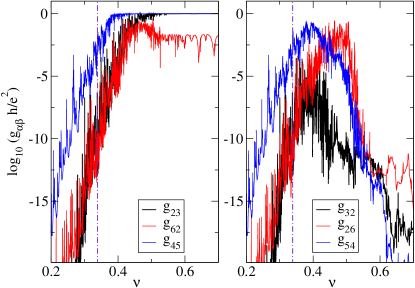
Figure 2: (color online) Representative conductance matrix elements, in units of $e^{2}/h$, as a function of the filling factor $\nu$. The left (right) panel shows $g_{23},g_{45}$ and $g_{62}$, respectively $g_{32}$, $g_{54}$ and $g_{26}$ characterizing transport in the (against the) direction of the edge currents. Results are almost identical on the left of the dot-dashed line, but different on its right.

Using the conductance matrix $\hat{g}(\nu)$ plotted in Fig. 2, we now compute the values of the various resistances as a function of $0<\nu<1$. Fig. 3(a) shows a pair $R_{L}$ and $R_{H}$. Three different regimes are clearly seen: for $\nu>0.46$, $R_{H}=h/e^{2}$ and $R_{L}=0$, corresponding to the first IQHE plateau. For $0.42<\nu<0.46$, $R_{L}$ exhibits large fluctuations, however $R_{H}$ is still well quantized. This is precisely the type of behavior observed in Ref. Peled1, . For $\nu<0.42$ the transition to the insulating phase occurs, and both resistances increase sharply. The fluctuations are very large and narrow because the calculation is done at $T=0$. At finite $T$, the peaks are smeared out.

The transition $1<\nu<2$ can also be simulated using the same $\hat{g}(\nu)$ matrix of the LLL. Similar to Ref. Shahar, , we assume that the completely filled spin-up LLL contributes its background chiral edge current. As a result, we simply add $\hat{g}^{(0)}=\hat{g}(\nu=1)$ of Eq. (1) to the values of $\hat{g}(\nu)$ describing the partially filled spin-down LLL. Although the two LLLs have different spins, the contacts mix electrons with both spins in equilibrium, justifying this addition. Resistivities $R^{H}_{14,62}$ and $R^{L}_{14,23}$ computed for $\hat{g}^{(0)}+\hat{g}(\nu)$ are shown in panel (b) of Fig. 3, whereas in panel (c) we plot their sum. The three regimes found experimentally Peled2 ; private are clearly observed. At low-$\nu$ (high-$B$), the fluctuations of $R_{H}$ and $R_{L}$ are correlated, $R_{L}+R_{H}=h/e^{2}$. At high-$\nu$ (low-$B$) $R_{H}=h/2e^{2}$ is quantized while $R_{L}$ still exhibits strong fluctuations. In the intermediate regime, both $R_{H}$ and $R_{L}$ have strong, uncorrelated fluctuations. The other pair, $R^{H}_{14,53}$ and $R^{L}_{14,65}$, also exhibits the three regimes, although their detailed fluctuations are different from $R^{H}_{14,62}$ and $R^{L}_{14,23}$. From over 20 different simulations we found that the low-$\nu$ regime where $R_{L}+R_{H}=h/e^{2}$ is a very robust feature, although it is maintained up to different values of $\nu$ in different samples. The high-$\nu$ regime with fluctuations in $R_{L}$ and quantized $R_{H}$ is seen frequently. However, when strong direct tunneling occurs between the source or the drain and their nearby voltage probes, $R_{H}$ also fluctuates. Such strong tunneling is an artifact of our simulation note1 . We suppress it by isolating the source and drain from nearby contacts with triangular potential barriers in the corners of the sample [see Fig. 1(a)]. Figure 3(c) also compares $R^{L}_{14,23}+R^{H}_{14,62}=R_{14,63}$ with $R_{2t}=R_{63,63}$. [In the setup for measuring $R_{2t}$, the current is $\hat{I}_{63}=\begin{pmatrix}0&0&1&0&0&-1\end{pmatrix}^{T}$, and $R_{2t}=V_{6}-V_{3}$]. As found experimentally Peled2 , the two curves are very similar.

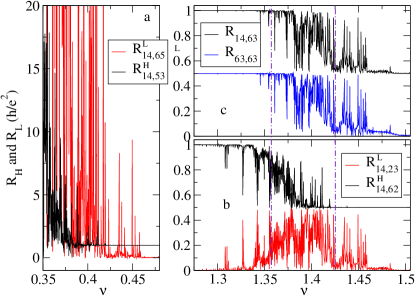
Figure 3: (color online) $R_{L}$ and $R_{H}$ calculated from the conductance matrix displayed in Fig. 2, in units of $h/e^{2}$. (a) Transition from the insulator to the first IQHE plateau in the LLL. (b) Transition from the first to the second IQHE plateaus. (c) The sum $R_{L}+R_{H}$ of the resistances shown in (b), and $R_{2t}-0.5{h/e^{2}}$. Vertical lines indicate the boundaries of the critical region. See text for further details.

So far, we have demonstrated that our numerical simulations recapture faithfully the experimental results. We now explain the underlying physics using a simple but very general model. For the given constraints and using logical induction, we find Zhou that $\hat{g}$ can be decomposed as a sum over loops connecting contacts: $\hat{g}=\sum c(k_{1},\cdots,k_{n})\hat{r}(k_{1},\cdots,k_{n})$. Here, $c$ are positive numbers and $\hat{r}(k_{1},\cdots,k_{n})=\hat{l}(k_{1},k_{2})+\dots+\hat{l}(k_{n},k_{1})$, where $l_{\alpha\beta}(a,b)=\frac{e^{2}}{h}\left(\delta_{\alpha a}\delta_{\beta b}-\frac{1}{2}\delta_{\alpha a}\delta_{\beta a}-\frac{1}{2}\delta_{\alpha b}\delta_{\beta b}\right)$ contributes to a single off-diagonal element $g_{ab}$. A two-vertex loop $\hat{r}(a,b)$ describes a $h/e^{2}$ resistor between contacts $a$ and $b$. Since ${r}_{\alpha\beta}(a,b)={r}_{\beta\alpha}(a,b)$, these terms are the symmetric part to $\hat{g}$. The asymmetric part of $\hat{g}$ describes chiral currents, whose direction of flow is dictated by the sign of $B$. In particular, $\hat{r}(1,2,3,4,5,6)=\hat{g}^{(0)}$ of Eq. 1 describes the edge currents of a LL, but shorter chiral circuits may also develop at intermediate fillings $\nu$.

At low-$\nu$, all states are localized and transport in the LL can only occur through tunneling. Consider the semi-classical case sketched on the left side of Fig. 1(c). Electrons can go from 2 to 1 either through direct tunneling (probability $t_{12}$), or they can tunnel to the localized state near contact 6 and from there back into 1, with probability $(1-t_{12})t_{26}t_{16}(1-t_{12})$. Electrons can make any number of loops before entering 1, the total sum being $p_{2\rightarrow 1}=\frac{h}{e^{2}}g_{12}=[t_{12}+t_{26}t_{16}-2t_{12}t_{26}t_{16}]/(1-t_{12}t_{16}t_{26})$. Similar arguments give $p_{1\rightarrow 2}=\frac{h}{e^{2}}g_{21}=[t_{12}-t_{26}t_{16}-t_{12}t_{16}]/(1-t_{12}t_{16}t_{26})$. $g_{16},g_{61},g_{26}$ and $g_{62}$ are computed similarly. We define $r_{ab}=\min(p_{a\rightarrow b},p_{b\rightarrow a})>0$, and $c_{ab}=\max(p_{a\rightarrow b},p_{b\rightarrow a})-r_{ab}>0$. We find $c_{12}=c_{26}=c_{61}=c=t_{12}t_{16}+t_{12}t_{26}+t_{16}t_{26}+O(t^{3})$; and up to $O(t^{2})$, $r_{12}\approx t_{12}$, $r_{16}\approx t_{16}$ and $r_{26}\approx t_{26}$. These processes contribute a total of $r_{12}\hat{r}(1,2)+r_{16}\hat{r}(1,6)+r_{26}\hat{r}(2,6)+c\hat{r}(1,2,6)$ to $\hat{g}$. The symmetric resistance terms, of order $t$, are due to direct tunneling between contacts, and at low-$\nu$ they dominate the small chiral current, of order $t^{2}$. This explains why for $\nu<\nu_{c}$, $\hat{g}$ is symmetric with small off-diagonal components (see Fig. 2). At high enough $\nu$, edge states connecting consecutive contacts appear. As already discussed, as $\nu\rightarrow 1$, $\hat{g}\rightarrow\hat{g}^{(0)}=\hat{r}(1,2,3,4,5,6)$. For intermediate $\nu$, shorter chiral loops containing edge states can be established through tunneling, as sketched on the right side of Fig. 2(c). Assume that an electron leaving contact 3 can tunnel with probabilities $t_{3}$ and $t_{5}$ to and out of a localized state, to join the opposite edge current and enter 5. It follows that $p_{3\rightarrow 5}=\frac{h}{e^{2}}g_{53}=t_{3}t_{5}/[1-(1-t_{3})(1-t_{5})]$, whereas $p_{5\rightarrow 3}=0$ (no electron leaving 5 enters 3). Then $r_{35}=0$ and the contribution to $\hat{g}$ is just $p_{3\rightarrow 5}\hat{l}(5,3)$. This term combines with parts of $\hat{l}(3,4)$ and $\hat{l}(4,5)$ to create a chiral current $c\hat{r}(3,4,5)$, where $c=p_{3\rightarrow 5}$. Physically, this represents the backscattered current of the Jain-Kivelson model Jain .

In general, one has to sum over many types of competing processes, involving both tunneling and edge states, but $\hat{g}$ can always be decomposed into symmetric resistances plus chiral loops. Consider the general form $\hat{g}=n\hat{g}^{(0)}+r_{12}\hat{r}(1,2)+r_{16}\hat{r}(1,6)+r_{26}\hat{r}(2,6)+r_{34}\hat{r}(3,4)+r_{45}\hat{r}(4,5)+r_{35}\hat{r}(3,5)+c_{0}\hat{g}^{(0)}+c_{1}\hat{r}(1,2,6)+c_{2}\hat{r}(2,3,5,6)+c_{3}\hat{r}(3,4,5)+c_{4}\hat{r}(1,2,3,5,6)+c_{5}\hat{r}(2,3,4,5,6)$. The first term describes the contribution of the $n$ completely filled lower LLs. All other terms describe transport in the LL hosting $E_{F}$ [see Fig. 1(b)], with the restriction that there is no tunneling between the left and right sides of the sample. This is justified physically because tunneling between contacts far apart is vanishingly small. The largest such terms, $r_{23}$ and $r_{56}$, are found to be less than $10^{-4}$ [see e.g. Fig. 2 , where $r_{23}=h/e^{2}\cdot\min(g_{32},g_{32})$]. We solve both $\hat{I}_{14}=\hat{g}\cdot\hat{V}$ and $\hat{I}_{63}=\hat{g}\cdot\hat{V^{\prime}}$ and find the identity

$$R_{14,63}=R_{63,63}=\frac{h}{e^{2}}\frac{1}{n+c_{0}+c_{2}+c_{4}+c_{5}}$$

Since $R_{63,63}=R_{2t}$, whereas $R_{14,63}=R^{H}_{14,62}+R^{L}_{14,23}=R^{L}_{14,65}+R^{H}_{14,53}$, this means that $R_{2t}=R_{H}+R_{L}$ irrespective of the value of the 12 parameters. In other words, this identity is obeyed for all $\nu$, in agreement with Fig. 3(c). (Adding $r_{23}$ and $r_{56}$ terms leads to perturbationally small corrections Zhou ). Here $n+c_{0}+c_{2}+c_{4}+c_{5}$ is the total chiral current flowing along the $6\rightarrow 5$ and $3\rightarrow 2$ edges. In particular, at low-$\nu$ chiral currents in the LL hosting $E_{F}$ are vanishingly small $c_{0}=c_{2}=c_{4}=c_{5}=0$ (there are no edge states established yet, and pure tunneling contributions are of order $t^{2}$, as already discussed. Below $\nu_{c}$, all $t<10^{-4}$, see Fig. 2). It follows that here $R_{L}+R_{H}=h/ne^{2}$, explaining the perfect correlations in the pattern fluctuations at low-$\nu$ of the two resistances, observed both experimentally and numerically.

The high-$\nu$ regime with quantized $R_{H}$ and fluctuating $R_{L}$ can also be understood easily. As already discussed, transport in the LL hosting $E_{F}$ is dominated here by the edge states; tunneling between opposite edge states (facilitated by localized states inside the sample) creates backscattered currents, as in the Jain-Kivelson model Jain . We sketch this situation in Fig. 1(d), where $t_{1}$, $t_{2}$ respectively $t_{3}$ include all possible tunneling processes leading to backscattering on the corresponding pairs of edge states. Reading the various probabilities off Fig. 1(d), we find that $\hat{g}=n\hat{g}^{(0)}+(1-t_{1}-t_{2}-t_{3})\hat{g}^{(0)}+t_{2}[\hat{r}(1,2,6)+\hat{r}(3,4,5)]+t_{3}\hat{r}(1,2,3,5,6)+t_{1}\hat{r}(2,3,4,5,6)$. The first term represents the contribution of the lower $n$ completely filled LLs, the others are the forward and the backscattered chiral currents in the LL hosting $E_{F}$. $\hat{I}_{14}=\hat{g}\cdot\hat{V}$ is trivial to solve. We find $R^{H}_{14,62}=R^{H}_{14,53}=h/(n+1)e^{2}$, i. e. the Hall resistances are precisely quantized, whereas $R^{L}_{14,23}=R^{L}_{14,65}=[h/(n+1)e^{2}]\cdot t_{2}/(n+1-t_{2})$. Since $t_{2}$ has a strong resonant dependence on $E_{F}$ (or $\nu$), it follows that $R_{L}$ fluctuates strongly. In particular, if $n=0$ (transition inside spin-up LLL), $R_{L}$ can be arbitrarily large when $t_{2}\rightarrow 1$, whereas in higher LLs the amplitude of fluctuations in $R_{L}$ is $h/(n+1)e^{2}$ or less, as observed both experimentally and in our simulations.

If $B$ changes sign, we have verified that the identity $\hat{g}(-B)=[\hat{g}(B)]^{T}$ holds Baranger . The reason is that time-reversal symmetric tunneling is not affected by this sign change, while the flow of the chiral currents is reversed. The model mirrors itself with respect to the horizontal axis if $B$ changes sign, see Fig. 1. The solutions of $\hat{I}_{14}=\hat{g}(-B)\cdot\hat{v}$ are then related to the solutions of $\hat{I}_{14}=\hat{g}(B)\cdot\hat{V}$ by $v_{2}=V_{6}$, $v_{3}=V_{5}$, $v_{5}=V_{3}$ and $v_{6}=V_{2}$, provided that the same index exchanges $2\leftrightarrow 6$, $3\leftrightarrow 5$, are performed for all $r_{ab}$. Terms not invariant under this transformation are $r_{12}$, $r_{16}$, $r_{43}$, $r_{45}$, $r_{23}$ and $r_{56}$. As already discussed, the last two terms are vanishingly small. In the experimental setup, the first four terms are also very small, due to the long distance between source and drain, and their nearby contacts note1 . The dominant terms $r_{26}$ and $r_{35}$ are invariant under the index exchange. It follows then that $R^{L}_{14,23}(B)=R^{L}_{14,65}(-B)$ and vice versa, i. e. with good accuracy, the fluctuation pattern of one $R_{L}$ mirrors that of the other $R_{L}$ when $B\rightarrow-B$. This symmetry has indeed been observed experimentally, with small violations at low-$\nu$ private due to perturbative corrections from the non-invariant tunneling contributions $r_{12}-r_{16}$ and $r_{43}-r_{45}$.

We now summarize our understanding of the various results of IQHE measurements on mesoscopic samples. Similar to experiments, we find that the transition in higher LLs is naturally divided in three regimes. At low-$\nu$, the LL hosting $E_{F}$ is insulating and there are no edge states connecting the left and right sides of the sample. If tunneling between left and right sides is also small, we find that the fluctuations of pairs of resistances are correlated with excellent accuracy, $R_{H}+R_{L}=h/ne^{2}$. This condition is obeyed if the typical size of the wave-function (localization length) is less than the distance between contacts 2 and 3. When the localization length becomes comparable to this distance, an edge state is established and the correlation between $R_{L}$ and $R_{H}$ is lost. On the high-$\nu$ side the edge states are established, but localized states inside the sample can help electrons tunnel between opposite edges, leading to back-scattering like the Jain-Kivelson model. In this case, we showed that $R_{L}$ fluctuates while $R_{H}$ is quantized. Tunneling between opposite edges is likely only if the typical size of the wave-functions is slightly shorter than the distance between opposite edges. It is then apparent that the central regime in Figs. 3 (b) and (c) corresponds to the so-called “critical region”, where the typical size of the electron wave-function is larger than the sample size (distance between contacts 2 and 3, at low-$\nu$, or between 2 and 6 at high-$\nu$). In these mesoscopic samples, the voltage probes act as markers on a ruler, measuring the localization length of the wave-functions at the Fermi energy. To our knowledge, this is the first time when the boundaries of the critical region are pinpointed experimentally. This opens up exciting possibilities for experimentally testing the predictions of the localization theory.

To conclude, we used both first-principles simulations and a simple model to explain the phenomenology of the mesoscopic IQHE, for six-terminal geometry. We identified tunneling and chiral currents as coexisting mechanisms for charge transport in mesoscopic samples, and argued that the boundaries between the three distinct regimes mark the critical region.

This research was supported by NSERC and NSF DMR-0213706. We thank Y. Chen, R. Fisch, R. N. Bhatt and D. Shahar for helpful discussions.

References

- (1) E. Peled et. al., Phys. Rev. Lett. 90, 246802 (2003).
- (2) E. Peled et. al., to appear in Phys. Rev. Lett.; cond-mat/0307423.
- (3) A. M. Chang et. al., Solid State Commun. 76, 769 (1988); G. Timp et. al., Phys. Rev. Lett. 59, 732 (1987).
- (4) J. A. Simmons et. al., Phys. Rev. Lett. 63, 1731 (1989).
- (5) D. H. Cobden et. al., Phys. Rev. Lett. 82, 4695 (1999).
- (6) S. Cho and M. P. A. Fisher, Phys. Rev. B, 55, 1637 (1997).
- (7) P. Streda et. al., Phys. Rev. Lett. 59, 1973 (1987).
- (8) J. K. Jain and S. A. Kivelson, Phys. Rev. Lett. 60, 1542 (1988).
- (9) M. Büttiker, Phys. Rev. Lett. 62, 229 (1989).
- (10) M. Büttiker, Phys. Rev. Lett. 57, 1761 (1986); Phys. Rev. B 38, 9375 (1988).
- (11) H. U. Baranger and A. D. Stone, Phys. Rev. B 40, 8169 (1989).
- (12) C. Zhou and M. Berciu, in preparation.
- (13) D. Shahar et. al., Phys. Rev. Lett. 79, 479 (1997).
- (14) Y. Chen and D. Shahar (private communication).
- (15) We use short samples (mm) in order to save CPU time by decreasing the number of states in the LLL; experimental devices are much longer (mm).