Quench dynamics across quantum critical points

Abstract

We study the quantum dynamics of a number of model systems as their coupling constants are changed rapidly across a quantum critical point. The primary motivation is provided by the recent experiments of Greiner et al. (Nature 415, 39 (2002)) who studied the response of a Mott insulator of ultracold atoms in an optical lattice to a strong potential gradient. In a previous work, it had been argued that the resonant response observed at a critical potential gradient could be understood by proximity to an Ising quantum critical point describing the onset of density wave order. Here we obtain numerical results on the evolution of the density wave order as the potential gradient is scanned across the quantum critical point. This is supplemented by studies of the integrable quantum Ising spin chain in a transverse field, where we obtain exact results for the evolution of the Ising order correlations under a time-dependent transverse field. We also study the evolution of transverse superfluid order in the three dimensional case. In all cases, the order parameter is best enhanced in the vicinity of the quantum critical point.

I Introduction

Recent experiments with ultracold atoms have achieved reversible tuning of bosonic atoms between superfluid and Mott insulating states by varying the strength of periodic potential produced by standing laser light Bloch ; Kasevich . The physics of such ultracold atoms in the Mott insulating state can be described by bosonic Hubbard model, well known in context of other condensed matter systems fwgf ; Sachdev1 . However, ultracold atoms in optical lattices offer much better control over microscopic parameters of the model. Consequently, it is possible to explore parameter regimes which are not available in other analogous condensed matter systems.

This paper will focus on a particular experiment reported by Greiner et al. Bloch . With the boson system in the Mott insulating state, they applied a steep potential gradient to the lattice, and observed its response. In a typical condensed matter system, one might have expected a response analogous to that of a sliding charge density wave: no motion of atoms until a critical tilt was applied, and a sliding motion at all tilts above the critical tilt. However, the experiment observed strikingly different behavior: there was a strong resonant response in the vicinity of tilts where the potential energy drop between nearest neighbor optical lattice sites ($E$) equaled the repulsion between two atoms on the same site ($U$). For $E\sim U$, applying the tilt produced a noticeable change in the ground state, but (in contrast to sliding charge density wave systems), there was little change in the ground state for larger $E$ until a second resonant peak at $E\sim 2U$. This resonant response is a clear indication that the atoms experience little extrinsic dissipation, and their dynamics should be described by an energy-conserving quantum Hamiltonian.

A framework for describing the experiments of Greiner et al. Bloch was proposed in Ref. Sachdev2, (hereafter referred to as I). (We also note here the numerical studies of Braun-Munzinger et al. burnett which addressed these experiments by studying the time evolution of the underlying Bose-Hubbard model.) For $w,|E-U|\ll E,U$, where $w$ is the tunnelling matrix element between nearest neighbor lattice sites, it was argued that we need only focus on a set of states which were resonantly coupled to the original Mott insulating state. In one dimension, the resonant subspace could be described simply in terms of nearest neighbor dipole states, consisting of a particle and a hole excitation about the Mott insulator on nearest neighbor states; in higher-dimensions, the particle and hole were no longer constrained to be on nearest-neighbor sites but could reside anywhere on planes orthogonal to the potential gradient, but separated by a single lattice spacing. An effective Hamiltonian on such resonant subspaces was proposed in I, and its phase diagram was presented. In the regime of large potential gradient $E-U>w$, this effective Hamiltonian possessed ground states with density wave order with a period of 2 lattice spacings (see also Ref. fendley, for conditions under which other periods may obtain). It was argued in I that the proximity of the quantum critical point, associated with the onset of this density wave order, was responsible for the resonant response observed by Greiner et al..

The tilt experiments of Greiner et al. were carried out in highly non-equilibrium situations, and the approach of I was to describe these, to the extent possible, by an equilibrium analysis of an effective Hamiltonian describing the primary states accessed over the experimental time scale. The purpose of the present paper is to directly address the non-equilibrium dynamics of the tilted Mott insulator. We will mainly do this using the effective Hamiltonian of I. The specific question we shall address is the following. Begin with the system in the ground state in a regime of small $E=E_{i}$ where there is no density wave order. Then, suddenly change the value of $E$ to a $E=E_{f}$, including values such that the ground state has density wave order at $E_{f}$. Allow the system to evolve under the resulting Hamiltonian. What is the nature of the state to which the system evolves at long times? We will find, as conjectured in I, that the density wave order that develops under this dynamic evolution is most robust when $E_{f}$ is near the quantum critical point.

We will also address a similar question for the Ising chain in a transverse field, $g$. Like the models of I, this model also has a regime, $g<g_{c}$, where the ground state has spontaneous Ising order. However, this much simpler model is completely integrable, and so offers an opportunity to analyze the non-equilibrium dynamics exactly. We initialize the Ising model in the ground state in a transverse field $g_{i}>g_{c}$. The transverse field is then changed rapidly to $g=g_{f}$, and the wavefunction evolves at this field. We will compute equal-time correlations in this wavefunction as a function of the time $t$, including in the $t\rightarrow\infty$ limit. In some cases, exact closed-form results will be obtained. The structure of these correlations as a function of $g_{f}$ bear some similarity to the results of the model of I as a function of $E_{f}$; however, there are some interesting differences which, we suspect, are related to the integrability of the Ising chain.

We now outline the remainder of the paper. In Section II we present numerical results on the dynamics of the one-dimensional dipole model of I. Section III will address the non-equilibrium dynamics of the Ising chain in a transverse field: this analysis uses the Jordan-Wigner transformation, and obtains the required dynamic correlation functions in the form of Toeplitz determinants. Section IV returns to the model of I, but turns to the dynamics in three dimensions; here, we use a combination of mean-field theory and exact diagonalization to obtain results similar to those in Section II, but with the order parameter now being a ‘transverse superfluid’ order. We review the results and discuss implications for experiments in Section V.

II Dipole dynamics in one dimension

This section will describe our numerical results on the quantum dynamics of the one-dimensional dipole model of the Mott insulator in a potential gradient.

Starting from a parent Mott state with $n_{0}$ bosons per site, we identified the set of states which are resonantly coupled to the parent Mott state when $U\sim E$ (recall that $U$ is the repulsive energy between two bosons on the same site, and $E$, the ‘electric field’, is the potential drop between two nearest neighbor sites). In one dimension, the resonant subspace involves dipole states consisting of quasihole-quasiparticle pairs at adjacent sites, and the low energy behavior of the system can be described by the effective dipole Hamiltonian obtained in I:

$$H_{\rm 1D}[E] = -w\sqrt{n_{0}(n_{0}+1)}\sum_{\ell}(d_{\ell}^{\dagger}+d_{\ell})$$ (1)

$$+(U-E)\sum_{\ell}d_{\ell}^{\dagger}d_{\ell}.$$

The dipoles are subject to hardcore constraints that there is never more than a single dipole on any pair of nearest neighbor sites

$$d_{\ell}^{\dagger}d_{\ell}\leq 1~{}~{}~{};~{}~{}~{}d_{\ell+1}^{\dagger}d_{\ell+1}d_{\ell}^{\dagger}d_{\ell}=0.$$ (2)

When the electric field $E$ is adiabatically tuned through $U$, the ground state of the system changes from one with no dipoles ($U\gg E$) to one with maximum possible number of dipoles ($E\gg U$). At an intermediate critical electric field

$$E_{c}=U+1.310w\sqrt{n_{0}(n_{0}+1)},$$ (3)

the system undergoes a quantum phase transition in the Ising universality class.

As discussed in Section I, we study the dynamics of the ultracold atoms when the potential gradient is changed suddenly. Such a situation can be very easily achieved experimentally in these systems by rapidly shifting the center of the confining magnetic trap. We shall specifically consider the situation where the change in the potential gradient is fast enough for the sudden perturbation assumption to be valid but slow enough to restrict the dynamics within the resonant subspaces so that the Hamiltonians (1) (and (LABEL:ham3d) in Section IV) are still valid.

We assume that the atoms in the 1D lattice are initially in the ground state $|\Psi_{G}\rangle$ of the dipole Hamiltonian (1) with $E=E_{i}\ll E_{c}$. This ground state corresponds to dipole vacuum. Consider shifting the center of the magnetic trap so that the new potential gradient is $E_{f}$. If this change is done suddenly, the system initially remains in the old ground state. The state of the system at time $t$ is therefore given by

$$|\Psi(t)\rangle=\sum_{n}c_{n}\exp(-i\epsilon_{n}t/\hbar)|n\rangle,$$ (4)

where $|n\rangle$ denotes the complete set of energy eigenstates of the Hamiltonian $H_{\rm 1D}[E_{f}]$ in (1), $\epsilon_{n}=\,\,\langle n|H_{\rm 1D}[E_{f}]|n\rangle$ is the energy eigenvalue corresponding to state $|n\rangle$, and $c_{n}=\,\,\langle n|\Psi(t=0)\rangle=\langle n|\Psi_{G}\rangle$ denotes the overlap of the old ground state with the state $|n\rangle$. Notice that the state $|\Psi(t)\rangle$ is no longer the ground state of the new Hamiltonian. Furthermore, in the absence of any dissipative mechanism, which is the case for ultracold atoms in optical lattices, $|\Psi(t)\rangle$ will never reach the ground state of the new Hamiltonian. Rather, in general, we expect the system to thermalize at long enough times, so that the correlations are similar to those of $H_{\rm 1D}[E_{f}]$ at some finite temperature.

We are now in a position to study the dynamics of the Ising density wave order parameter

$$O=\frac{1}{N}\langle\Psi|\sum_{\ell}(-1)^{\ell}d_{\ell}^{\dagger}d_{\ell}|\Psi\rangle,$$ (5)

where $N$ is the number of sites. The time evolution of $O$ is given by

$$O(t) = \frac{1}{N}\sum_{m,n}c_{m}c_{n}\cos\left[\left(E_{m}-E_{n}\right)t/\hbar\right]$$ (6)

$$\times\langle m|\sum_{\ell}(-1)^{\ell}d_{\ell}^{\dagger}d_{\ell}|n\rangle$$

Eq. 6 is solved numerically using exact diagonalization to obtain the eigenstates and eigenvalues of the Hamiltonian $H_{\rm 1D}[E_{f}]$. Before resorting to numerics, it is however useful to discuss the behavior of $O(t)$ qualitatively. We note that if $E_{f}$ is close to $E_{i}$, the old ground state will have a large overlap with new one $\it i.e.$ $c_{m}\sim\delta_{m1}$. Hence in this case we expect $O(t)$ to have small oscillations about $O(t=0)$. On the other hand, if $E_{f}\gg E_{c}$, the two ground states will have very little overlap, and we again expect $O(t)$ to have a small oscillation amplitude. This situation is in stark contrast with the adiabatic turning on of the potential gradient, where the systems always remain in the ground state of the new Hamiltonian $H_{\rm 1D}[E_{f}]$, and therefore has a maximal value of $\langle O\rangle$ for $E_{f}\gg E_{c}$. In between, for $E_{f}\sim E_{c}$, the ground state $|\Psi\rangle$ has a finite overlap with many states $|m\rangle$, and hence we expect $O(t)$ to display significant oscillations. Furthermore, if the symmetry between the two Ising ordered states is broken slightly (as is the case in our studies below), the time average value of $O(t)$ will be non-zero.

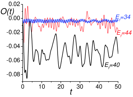
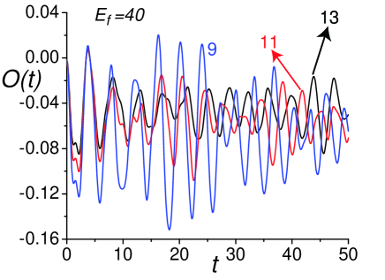
This qualitative discussion is supported by numerical calculations on finite size systems for system size $N=9,11,13$. For numerical computations with finite systems, we choose systems with an odd number of sites and open boundary conditions, so that dipole formation on odd sites is favored, thus breaking the $Z_{2}$ symmetry. The results are shown in Figs. 1- 4.

Figure 1: Evolution of the Ising order parameter in (5) under the Hamiltonian $H_{\rm 1D}[E_{f}]$ for $n_{0}=1$. The initial state is the ground state of $H_{\rm 1D}[E_{i}]$. All the plots in this section have $U=40$, $w=1$, and $E_{i}=32$, and consequently the equilibrium quantum critical point is at $E_{c}=41.85$.

Figure 2: System size ($N$) dependence of the results of Fig 1 for $E_{f}=40$. The curves are labelled by the value of $N$.

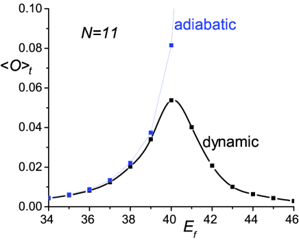
Figure 3: The curve labelled ‘dynamic’ is the long time limit, $\langle O\rangle_{t}$ of the Ising order in (6) as a function of $E_{f}$ (for $N=11$), with other parameters as in Fig 1. This long time limit can be obtained simply by setting $m=n$ in (6). For comparison, in the curve labelled ‘adiabatic’, we show the expectation value of the Ising order $O$ in the ground state of $H_{\rm 1D}[E_{f}]$; such an order would be observed if the value of $E$ was changed adiabatically. Note that the dynamic curve has its maximal value near (but not exactly at) the equilibrium quantum critical point $E_{c}=41.85$, where the system is able to respond most easily to the change in value of $E$; this dynamic curve is our theory of the ‘resonant’ response in the experiments of Ref. Bloch, discussed in Section I. In contrast the adiabatic result increases monotonically with $E_{f}$ into the $E>E_{c}$ phase where the Ising symmetry is spontaneously broken.

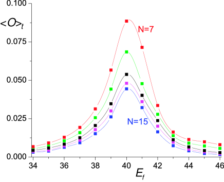
Figure 4: Size dependence of the ‘dynamic’ results in Fig 3. The sizes range from $N=7$ to $N=15$ (as labeled), with the intermediate values $N=9,11,13$: $\langle O\rangle_{t}$ decreases monotonically with $N$

Fig. 1 shows the oscillation of the order parameter $O(t)$ for different values of $E_{f}$ for $N=13$. In agreement with our qualitative expectations, the oscillations have maximum amplitude when $E_{f}\approx 40$ is near the critical value $E_{c}=41.85$. For either $E_{f}\ll E_{c}$ or $E_{f}\gg E_{c}$, the oscillations have a small amplitude around $O(t=0)$. Furthermore, it is only for $E_{f}\approx E_{c}$ that the time-average value of $O(t)$ is appreciable. Fig. 2 shows the system size dependence of the time evolution for $E_{f}=U=40$. We find that the oscillations remain visible as we go to higher system sizes, although they do weaken somewhat. More significantly, the time average value of $O(t)$ remains non-zero, and has a weaker decrease with system size. In Fig. 3, we plot the long time limit of the Ising order parameter, $\langle O\rangle_{t}$, as a function of $E_{f}$, and compare it with the $O_{\rm ad}$, the value of the order parameter when $E$ reaches $E_{f}$ adiabatically and the wavefunction is that of the ground state at $E=E_{f}$. We find that $\langle O\rangle_{t}$ stays close to $O_{\rm ad}$ as long as there is a large overlap with between the old and the new ground states. However, as we approach the adiabatic phase transition point, this overlap decreases and $\langle O\rangle_{t}$ can not follow $O_{\rm ad}$ any more. The deviation of $\langle O\rangle_{t}$ is therefore a signature that the system is now in a different phase for the new value of the electric field.

The ‘dynamic’ curve in Fig 3 should be compared with Figs 5e,f in Ref. Bloch, . The latter show that the Mott insulator has a resonantly strong response to an applied potential gradient $E\sim U$. Here, we have found a similar resonant enhancement in a simple model system in one dimension, induced by the proximity of a quantum critical point.

We comment briefly on the nature of the thermodynamic limit, $N\rightarrow\infty$ for the results in Fig 2, 3. For $O_{\rm ad}$ it is clear that there is a non-zero limit only for $E>E_{c}$, when it equals the order parameter of the spontaneously broken Ising symmetry. If we assume that the system thermalizes at long times for the dynamic case, then $\langle O\rangle_{t}$ corresponds to the expectation value of the equilibrium order parameter in $H_{1D}[E_{f}]$ at some finite temperature. In one dimension, it is not possible to break a discrete symmetry at finite temperatures, and so the thermodynamic limit of the order parameter must always vanish. By this reasoning, we expect $\langle O\rangle_{t}$ to also vanish in the thermodynamic limit. This is consistent with the results in Fig. 4, where we show the $N$ dependence of the long time limit $\langle O\rangle_{t}$. Our data are at present not extensive enough to definitely characterize the dependence of $\langle O\rangle_{t}$ on $N$.

III Dynamics of the quantum Ising chain

As a complement to the physically relevant, but numerical, computations in Section II, this section will describe similar results in a simpler, analytically tractable model. We will consider the integrable Ising chain in a transverse field, which also has a zero temperature, quantum phase transition between a phase with a broken $Z_{2}$ symmetry and a symmetric phase. We will address questions on the evolution of the wavefunction under a time-dependent change in the transverse field.

The model of interest in this section is

$$H_{I}=-J\sum_{j}\left(\sigma^{z}_{j}\sigma^{z}_{j+1}+g(t)\sigma^{x}_{i}\right),$$ (7)

where $\sigma^{x,z}_{j}$ are Pauli matrices acting on a ‘spin’ on the sites, $j$, of an infinite chain. We have allowed the transverse field to acquire an arbitrary time dependence $g(t)$. We will mainly consider here the case of a sudden change at time $t=0$ from an initial value $g(0^{-})=g_{i}$ to a final value $g(0^{+})=g_{f}$, but our methods easily generalize to the arbitrary time dependence in $g(t)$.

For time-independent $g(t)$, $H_{I}$ has a quantum critical point at $g=g_{c}=1$, with two equivalent ground states for $g<g_{c}$ related by a global $Z_{2}$ spin-flip. However, unlike Section II we will not introduce any external perturbation which introduces a preference between these two states: all such perturbations destroy the integrability of $H_{I}$. Consequently, we do not obtain any useful information from the analog of the time-dependence of the order parameter in (5), (6), as these quantities will be identically zero at all times. Rather, we will compute here the two-point correlation function of the order parameter in an infinite chain, which is

$$G_{n}(t)=\langle\psi(t)|\sigma^{z}_{j}\sigma^{z}_{j+n}|\psi(t)\rangle.$$ (8)

Here $|\psi(t)\rangle$ is the state of the system at time $t$, evolving under the Schödinger equation specified by the time-dependent Hamiltonian $H_{I}$. In equilibrium, the information contained in a correlation function like (8) is related to an observable like that in (6) (which is the response in the Ising order parameter to perturbations in the boundary condition) by the fluctuation-dissipation theorem. However, we are not aware of any analog of such a theorem for the non-equilibrium case under consideration here, and so are not able to directly relate the results of the present section to those of Section II.

Our analysis of $H_{I}$ proceeds with the standard Jordan-Wigner transformation, and we follow the notation and methods of Chapter 4 of Ref. Sachdev1, . We express the $S=1/2$ states in terms of those of the spinless Jordan-Wigner fermion $c_{j}$, and after transforming to momentum space fermions $c_{k}$, the Hamiltonian becomes

$$H_{I} = J\sum_{k}\left[2\left(g-\cos k\right)c_{k}^{\dagger}c_{k}\right.$$ (9)

$$~{}~{}~{}~{}~{}~{}~{}~{}~{}~{}\left.-i\sin k\left(c^{\dagger}_{-k}c_{k}^{\dagger}+c_{-k}c_{k}\right)-g\right].$$

Now, transforming to the Heisenberg picture, we can follow the evolution of the system by solving the equations of motion

$$\frac{dc_{k}}{dt}=i\left[H_{I},c_{k}\right].$$ (10)

These equations are easily solved by a Bogoliubov transformation. Finally, the correlator in (8) is computed by a simple generalization of the methods appropriate for the equilibrium case. A few details of such a computation appear in the Appendix.

Here, we discuss the results for $G_{n}(t)$ for the case of a sudden change from $g(0^{-})=g_{i}$ to $g(0^{+})=g_{f}$. For $t<0$, we assume the system is in the ground state appropriate for $g=g_{i}$, and consequently $G_{n}(t<0)$ is independent of $t$ and equal to the well-known equilibrium result at $g=g_{i}$. For $t>0$, there is a non-trivial time dependence, and it is possible to obtain the general expression for $G_{n}(t)$ as described in the Appendix. We will restrict our attention here to the simpler expression of the long time limit $G_{n}(t\rightarrow\infty)$, which is the primary quantity of physical interest. For this, we obtain the Toeplitz determinant

$$G_{n}(\infty)=\begin{vmatrix}a_{0}&a_{-1}&\ldots&a_{-n+1}\\ a_{1}&a_{0}&\ldots&a_{-n+2}\\ \vdots&\vdots&\ddots&\vdots\\ a_{n-1}&a_{n-2}&\ldots&a_{0}\end{vmatrix},$$ (11)

where

$$a_{r}=\frac{1}{2\pi}\int_{-\pi}^{\pi}e^{-ikr}\tilde{a}(k),$$ (12)

with

$$\tilde{a}(k) = \frac{2(g_{f}g_{i}+1)z-(g_{f}+g_{i})(z^{2}+1)}{2(z-g_{f})}$$ (13)

$$~{}~{}~{}~{}~{}~{}~{}~{}~{}~{}~{}\times\sqrt{\frac{z}{(z-g_{i})(1-zg_{i})}},$$

where $z=e^{ik}$.

We now need to evaluate the $n\times n$ Toeplitz determinant in (11), especially for the case of large $n$. In the equilibrium situation, this is aided by Szegö’s lemma, and its generalization in the Fisher-Hartwig formula fh . For the present situation, the expression in (13) does not obey the winding number constraint required for application of the Fisher-Hartwig formula, and so we are unable to take advantage of this result. However, we shall show that an exact evaluation of (11) is possible for two important special cases ($g_{i}=\infty$ and $g_{i}=0$), and supplement these by numerical evaluation of (11) for other values of $g_{i}$.

In the case $g_{i}=0$, we have

$$\tilde{a}(k)=\frac{2z-g_{f}(z^{2}+1)}{2(z-g_{f})}$$ (14)

and it is straightforward to evaluate $a_{r}$ by contour integration. This gives

$$\begin{array}[]{c|c|c}&g_{f}<1&g_{f}>1\\ \hline\cr\rule[-11.38109pt]{0.0pt}{31.29802pt}r\leq-1&\displaystyle\frac{g_{f}^{-r}}{2}(1-g_{f}^{2})&0\\ \hline\cr\rule[-11.38109pt]{0.0pt}{31.29802pt}r=0&1-\displaystyle\frac{g_{f}^{2}}{2}&\displaystyle\frac{1}{2}\\ \hline\cr\rule[-11.38109pt]{0.0pt}{31.29802pt}r=1&-\displaystyle\frac{g_{f}}{2}&-\displaystyle\frac{1}{2g_{f}}\\ \hline\cr\rule[-11.38109pt]{0.0pt}{31.29802pt}r\geq 2&0&\displaystyle\frac{g_{f}^{-r}}{2}(g_{f}^{2}-1)\end{array}~{}~{}.$$ (15)

For the case $g_{i}=+\infty$, we have

$$\tilde{a}(k)=\frac{2g_{f}z-(z^{2}+1)}{2(z-g_{f})}$$ (16)

and $a_{r}$ is given by

$$\begin{array}[]{c|c|c}&g_{f}<1&g_{f}>1\\ \hline\cr\rule[-11.38109pt]{0.0pt}{31.29802pt}r\leq-1&\displaystyle-\frac{g_{f}^{-r-1}}{2}(1-g_{f}^{2})&0\\ \hline\cr\rule[-14.22636pt]{0.0pt}{31.29802pt}r=0&\displaystyle\frac{g_{f}}{2}&\displaystyle\frac{1}{2g_{f}}\\ \hline\cr\rule[-14.22636pt]{0.0pt}{31.29802pt}r=1&\displaystyle-\frac{1}{2}&\displaystyle\frac{1}{2g_{f}^{2}}-1\\ \hline\cr\rule[-14.22636pt]{0.0pt}{31.29802pt}r\geq 2&0&\displaystyle-\frac{1}{2g_{f}^{r+1}}(g_{f}^{2}-1)\end{array}~{}~{}.$$ (17)

In both of these two cases, the following conditions are met:

Condition 1

For $g_{f}>1$, $a_{r}=0$ for $r\leq-1$.

Condition 2

For $g_{f}<1$, $a_{r}=0$ for $r\geq 2$.

Condition 3

For $g_{f}<1$, $a_{r}=ga_{r+1}$ for $r\leq-2$.

Using Condition 1, we can immediately write $G_{n}(\infty)=a_{0}^{n}$ for $g_{f}>1$. For $g_{f}<1$, define

$$D_{n}^{r}=\begin{vmatrix}a_{-r}&a_{-r-1}&\ldots&a_{-r-n+1}\\ a_{1}&a_{0}&\ldots&a_{-n+2}\\ \vdots&\vdots&\ddots&\vdots\\ a_{n-1}&a_{n-2}&\ldots&a_{0}\end{vmatrix},$$ (18)

so that $G_{n}(\infty)=D_{n}^{0}$. Condition 2 gives $D_{n}^{r}=a_{-}rD_{n-1}^{0}-a_{1}D_{n-1}^{r+1}$ and Condition 3 gives $D_{n}^{r}=g_{f}D_{n}^{r-1}$ for $r\geq 2$. Also, $D_{1}^{r}=a_{-r}$. We can therefore write

$$\begin{pmatrix}D_{n}^{0}\\ D_{n}^{1}\end{pmatrix} = \begin{pmatrix}a_{0}&-a_{1}\\ a_{-1}&-a_{1}g_{f}\end{pmatrix}\begin{pmatrix}D_{n-1}^{0}\\ D_{n-1}^{1}\end{pmatrix}$$ (19)

$$= {\begin{pmatrix}a_{0}&-a_{1}\\ a_{-1}&-a_{1}g_{f}\end{pmatrix}}^{n-1}\begin{pmatrix}D_{1}^{0}\\ D_{1}^{1}\end{pmatrix}$$ (20)

$$= {\begin{pmatrix}a_{0}&-a_{1}\\ a_{-1}&-a_{1}g_{f}\end{pmatrix}}^{n}\begin{pmatrix}1\\ 0\end{pmatrix}.$$ (21)

This can be evaluated by diagonalizing the matrix.

Collecting all the analytic results above, we have for the case $g_{i}=0$:

$$G_{n}(\infty)=\left\{\begin{array}[]{r}\displaystyle\frac{g_{f}^{n+1}}{2^{n}}\cosh\left[(n+1)\ln\left(\frac{1+\sqrt{1-g_{f}^{2}}}{g_{f}}\right)\right],\\ \mbox{for $g_{f}\leq 1$}\\ {}\hfil\\ \displaystyle\left(\frac{1}{2}\right)^{n},~{}~{}~{}~{}~{}~{}~{}~{}~{}~{}~{}\mbox{for $g_{f}\geq 1$}\end{array}\right.$$ (22)

In the limit that $n\rightarrow\infty$, the result for $g_{f}<1$ becomes

$$G_{n}(\infty)\rightarrow{\left(\frac{1+\sqrt{1-g_{f}^{2}}}{2}\right)}^{n+1}.$$ (23)

In the case $g_{i}=+\infty$, the corresponding results are

$$G_{n}(\infty)=\left\{\begin{array}[]{cc}\displaystyle\left(\frac{1}{2}\right)^{n}\cos\left(n\arccos(g_{f})\right),&\mbox{for $g_{f}\leq 1$}\\ {}\hfil\\ \displaystyle\left(\frac{1}{2g_{f}}\right)^{n},&\mbox{for $g_{f}\geq 1$}\end{array}\right.$$ (24)

Note that there are spatial oscillations in the correlator for the case where the field is reduced from a large positive value ($g_{i}=+\infty$) to a value below the critical point ($g_{f}<1$).

Of these exact results, the case $g_{i}=\infty$ is the one that corresponds most closely to the physical situation discussed in Section II. Here we start from an fully ‘disordered’ initial state, and then suddenly change parameters to values with increasing order (this is the analog of increasing $E$ in Section II). For final parameter values $g_{f}>g_{c}=1$, we find here a result quite similar to that found in Section II: from (24) we see that the order parameter correlations decay with the a correlation length $\xi_{f}$ given by

$$\xi_{f}=\frac{1}{\ln(2g_{f})}.$$ (25)

This increases monotonically with decreasing $g_{f}$, and is thus similar to the increase in the value of $\langle O\rangle_{t}$ with increasing $E_{f}$ for $E_{f}<E_{c}$ in Fig 3. By the analogy with Fig 3, we would expect here that there is a maximum in $\xi_{f}$ at $g=g_{c}$. However, we find a somewhat different behavior for $g_{f}<g_{c}$ in (24): the correlations do not decay in a simple exponential, but now oscillate, with the period of oscillation becoming smaller with decreasing $g_{f}$. So the correlations of the Ising ordered state are indeed best formed at $g_{f}=g_{c}$, but we find an unusual oscillatory decay of correlations for $g_{f}<g_{c}$. The oscillations are a clear indication of the absence of thermalization in the present model, and we expect they are special consequence of its integrability.

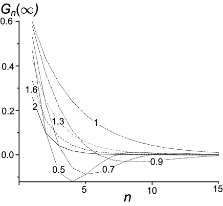
We extended these analytic results by numerical evaluation of (11) for other values of $g_{i}$, and found closely related behavior. Our results for $g_{i}=2$ are shown in Fig 5, and these are the analog here of the results in Fig 3 and 4.

Figure 5: Ising order correlations defined in (8). The system is in the ground state of $H_{I}$ for $t<0$ with $g=g_{i}=2$. At $t=0^{+}$, the value of $g$ is changed suddenly to $g=g_{f}$, and remains at this value for all $t>0$. Note that at long times, the order is best developed for $g_{f}=1$, which is the location of the equilibrium quantum critical point. This result is the analog of Figs 3 and 4 for the dipole model of Section II.

As $g_{f}$ is decreased, the correlations become longer-ranged, until they reach a maximum range at $g_{f}=g_{c}=1$. At smaller values of $g_{f}$, the correlations acquire an oscillatory behavior, but are also clearly shorter ranged. So the Ising order is best developed for $g_{f}$ near the quantum critical point.

IV Dynamics in three dimensions

We now return to the ‘tilted’ Mott insulator problem addressed in Section II and in I. Here we will address questions of quench dynamics for the three dimensional case. As discussed at length in I, the resonant subspace in 3D is described by quasiparticles and quasiholes which are free to move in the directions transverse to the applied electric field. Consequently, the dipoles of Section II, which are bound quasihole-quasiparticle pairs in adjacent sites, constitute only a small part of the resonant subspace, and an effective Hamiltonian for unbound quasiparticle and quasihole states is necessary. A mean-field theory of this effective Hamiltonian was examined in I, and a fairly complex phase diagram was found. In addition to the Ising density wave order that appeared in one dimension, states with a transverse superfluid order were present. The latter states correspond to delocalization of the quasiholes and quasiparticles in the direction transverse to the applied electric field.

In this section, we will address the quench dynamics across the transition associated with the onset of transverse superfluid order. This was found to be a second-order transition in the mean-field theory of I, and here we will extend the mean-field theory to an analysis of the non-equilibrium dynamics across the superfluid-insulator transition. We will not examine here the onset of Ising order, already studied in Section II; the present mean-field theory found a strong first-order transition for the onset of Ising order. Our analysis will be restricted to the regime where both the superfluid and insulating states have no Ising density wave order.

The effective mean-field Hamiltonian describing the dynamics of these quasiparticles and quasiholes can be written as in I:

$$H_{3D}[\langle p_{\ell}\rangle,\langle h_{\ell}\rangle;E]=$$

$$\sum_{\ell}\Bigg{[}-wZ\Big{(}n_{0}h_{\ell}\langle h_{\ell}\rangle^{*}+(n_{0}+1)p_{\ell}\langle p_{\ell}\rangle^{*}$$

$$+{\rm h.c}\Big{)}-w\sqrt{n_{0}(n_{0}+1)}\Big{(}p_{\ell}h_{\ell-1}+{\rm h.c}\Big{)}$$

$$+\frac{(U-E)}{2}\left(p_{\ell}^{\dagger}p_{\ell}+h_{\ell}^{\dagger}h_{\ell}\right)-\mu_{\ell}\left(p_{\ell+1}^{\dagger}p_{\ell+1}-h_{\ell}^{\dagger}h_{\ell}\right)\Bigg{]}.$$

Here $\ell$ is a one-dimensional site index labelling sites along the longitudinal direction of the applied potential gradient (the transverse degrees of freedom are treated in a mean-field approximation and so there is no dependence on the transverse site label), $p$ and $h$ are quasiparticle and quasihole annihilation operators, $Z$ is the number of nearest neighbors in the transverse directions and $\mu_{\ell}$ denotes chemical potential which enforces the constraints

$$\langle p_{\ell+1}^{\dagger}p_{\ell+1}\rangle=\langle h_{\ell}^{\dagger}h_{\ell}\rangle.$$ (27)

Although the Hamiltonian (LABEL:ham3d) has no non-linear terms, its diagonalization is non-trivial because of the hard-core constraint on all sites

$$p_{\ell}^{\dagger}p_{\ell}\leq 1,~{}~{}~{}~{}h_{\ell}^{\dagger}h_{\ell}\leq 1,~{}~{}~{}~{}p_{\ell}^{\dagger}p_{\ell}h_{\ell}^{\dagger}h_{\ell}=0.$$ (28)

The mean fields $\langle p_{\ell}\rangle$ and $\langle h_{\ell}\rangle$ correspond to transverse particle/hole superfluid order and were self consistently determined by diagonalizing the 3D Hamiltonian (LABEL:ham3d) while maintaining (28).

We now consider the evolution of the ground state under a sudden shift in the value of $E$ from $E=E_{i}$ to $E=E_{f}$ at $t=0^{+}$. We place $E_{i}$ in a regime where the ground state preserves all symmetry, and there is neither Ising or transverse superfluid order. The initial ground state $|\Psi^{\rm 3D}\rangle$ will evolve according to the new Hamiltonian $H_{\rm 3D}[\langle p\rangle,\langle h\rangle;E_{f}]$. However, in contrast to the 1D case, here the evolutions of the mean fields $\langle p\rangle$ and $\langle h\rangle$ have to be self-consistently determined. Within time-dependent Hartree approximation, we obtain

$$|\Psi^{\rm 3D}(t)\rangle = \sum_{m}c_{m}(t)|m\rangle$$

$$i\hbar\frac{dc_{m}(t)}{dt} = \sum_{n}c_{n}(t)$$

$$\times\langle n|H_{\rm 3D}[\langle p_{\ell}(t)\rangle,\langle h_{\ell}(t)\rangle;E_{f}]|m\rangle$$

$$\langle p_{\ell}(t)\rangle = \sum_{m,n}c_{m}^{*}(t)c_{n}(t)\langle m|p|n\rangle$$

$$\langle h_{\ell}(t)\rangle = \sum_{m,n}c_{m}^{*}(t)c_{n}(t)\langle m|h|n\rangle.$$ (29)

We used a basis of states $|n\rangle$ (the final results are, of course, independent of the choice of this basis) which are the complete set of eigenkets of the Hamiltonian $H_{\rm 3D}[\langle p_{\ell}^{f}\rangle,\langle h_{\ell}^{f}\rangle;E_{f}]$, where $\langle p_{\ell}^{f}\rangle$ and $\langle h_{\ell}^{f}\rangle$ are the ground states values of the particle and hole order condensates for $E=E_{f}$. All the states $|n\rangle$ maintain (28) exactly, and so these hard-core constraints are fully respected by our calculation: this is what makes diagonalization of the Hamiltonian time consuming and numerically intensive. We note that these equations also maintain the constraints (27) at all $\ell$ and $t$.

We examined the above equations for the transverse superfluid order using the same protocol used in Section II for the Ising order. The set of Eqs. 29 were solved self-consistently for longitudinal system size $N=4$. We consider the starting potential gradient $E_{i}$ to be in the insulator phase with neither superfluid or Ising order, and ramp up the potential gradient to enter the superfluid phase. The gauge symmetry of the superfluid order parameter is broken by adding a small symmetry breaking term $H_{\rm sym}=-\sum_{\ell}\eta[(p_{\ell}+h_{\ell})+{\rm h.c}]$, where $\eta$ is an infinitesimal positive constant. In the absence of such a symmetry breaking term we would have $\langle p_{\ell}\rangle$ and $\langle h_{\ell}\rangle$ vanish identically for all $t$ by gauge invariance. However, even an infinitesimal symmetry breaking is sufficient, in the suitable parameter regime, to induce appreciable values of the superfluid order. In practice, this symmetry breaking is provided by the coupling of the system to its environment.

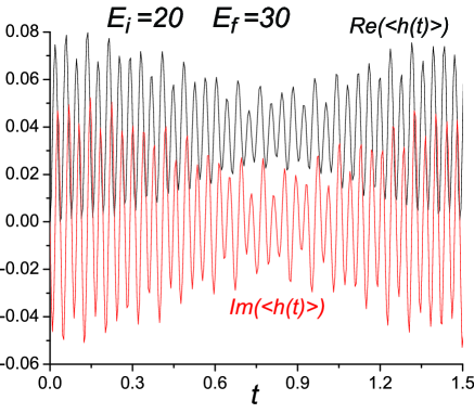
With the symmetry breaking term present, the superfluid order parameters $\langle p_{\ell}\rangle$ and $\langle h_{\ell}\rangle$ are initially real. As seen in Fig. 6, $\langle h(t)\rangle=\sum_{\ell}\langle h_{\ell}(t)\rangle$ develop coherent oscillations once the potential gradient takes the value $E_{f}$. (These results are the analog of Figs 1,2.)

Figure 6: Oscillations of the hole superfluid order parameter. The plot is shown for $U=40$, $w=1$, $n_{0}=1$, $Z=4$, $E_{i}=20$ and $E_{f}=30$. For these parameters, the quantum critical point is at $E_{c}=26.4$.

The oscillations in $\langle p(t)\rangle$ are similar, but occur with a different period due to the inherent particle-hole asymmetry in Eq. LABEL:ham3d. The long time average of the oscillations is purely real, and this is, of course determined by the symmetry breaking term. Such oscillations of the superfluid order parameter were also obtained recently in a different context in Refs. aa, ; psg, and by Levitov Levitov .

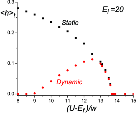
We also examined the $E_{f}$ dependence of the long time average of the superfluid order, and the analog of Fig 3 appears in Fig 7.

Figure 7: Analog of Fig 3, but for the transverse superfluid order, using the same parameters (apart from $E_{f}$) as Fig 4. The ”static” curve is the equilibrium superfluid order parameter determined in I. The ”dynamic” curve is the long time average of the real part of $\langle h(t)\rangle$.

Again the superfluid order is most strongly enhanced in the vicinity of the quantum critical point. However, unlike Fig 3, we do not observe a precursor to the superfluid order in the insulating phase: this is surely an artifact of the mean-field treatment of the transverse degrees of freedom.

V Conclusions

With advent of the study of quantum phase transitions in trapped atomic systems, there is a clear need for theoretical studies in the highly non-equilibrium situations that experiments are often in. In particular, experiments can easily explore the change in the state of the system upon a sudden change in a parameter in the Hamiltonian. There are few general principles in such cases (e.g. there is no fluctuation-dissipation theorem which controls correlations of the final state), and theory is clearly still in its infancy. Two recent studies in this class aa ; psg , examined the evolution of superfluid order under a sudden change in the optical lattice potential exerted on trapped bosons.

It is clear that exact results on simple solvable models in non-equilibrium situations would be valuable. We have provided such an example here in Section III, where we examined the Ising chain in a transverse field, $g$. This model has a quantum critical point at $g=g_{c}$, with spontaneous ferromagnetic order in the ground state for $g<g_{c}$. We started the Ising model in the paramagnetic state ($g_{i}\gg g_{c}$), suddenly at $t=0$ changed $g$ to a final value $g_{f}$, and examined the long time development of correlations of the ferromagnetic order. (Our formalism also provided results for all $t>0$, but we have not examined the detailed time evolution here.) The results are summarized in Fig 5. True long-range order does not develop at any value of $g_{f}$; however, significant order parameter correlations do appear, and these are best formed for $g_{f}\approx g_{c}$. In a general non-integrable system we may expect thermalization at long times, at a temperature such that the average energy equals that of the state at $t=0^{+}$. Such thermalization does not occur for the present integrable system, and the results have certain artifacts associated with this: the long-time correlations have an oscillatory spatial dependence for $g_{f}<g_{c}$.

In the remainder of the paper we studied the non-equilibrium dynamics of models introduced in a previous paper Sachdev2 which addressed the response of a bosonic Mott insulator to a change in a strong potential gradient Bloch . These models exhibit a number of quantum critical points associated with the onset of Ising density wave and superfluid order. Our numerical studies here found a feature similar to that also obtained for the solvable Ising model: the order was best formed when the final parameter value was in the vicinity of the associated quantum critical point, as illustrated in Fig 3. Here, and in Ref. Sachdev2, , we have proposed this feature as the explanation for the resonant response observed by Greiner et al. Bloch upon ‘tilting’ a Mott insulator of bosons in an optical lattice.

*

Appendix A Computations for the Ising chain

The Jordan-Wigner transformation allows the Hamiltonian of an Ising chain in a transverse field $g$ to be written as

$$H_{I}=\sum_{k}\epsilon_{k}\gamma_{k}^{\dagger}\gamma_{k},$$ (30)

where $\gamma_{k}$ is a fermionic annihilation operator (see Chapter 4 of Ref. Sachdev1, ). These are related to the Jordan-Wigner fermions $c_{k}$ by a Bogoliubov transformation, parametrized by angle $\theta_{k}$, where

$$\tan\theta_{k}=\frac{\sin k}{g-\cos k}.$$ (31)

In the present case, we define the $\gamma$ fermions as those that diagonalize the Hamiltonian for $t>0$, with field $g_{f}$.

Since the Hamiltonian is throughout translationally symmetric, only fermionic states with opposite pseudomomentum $k$ and $-k$ are mixed. We may therefore write the two component column vector

$$\Gamma_{k}=\begin{pmatrix}\gamma_{k}\\ \gamma_{-k}^{\dagger}\end{pmatrix}$$ (32)

and similarly $c_{k}$ for the Jordan-Wigner fermions. The Bogoliubov transformation relating $c_{k}$ and $\Gamma_{k}$ is expressed as $c_{k}=R^{x}(\theta_{k})\Gamma_{k}$, where

$$R^{x}(\alpha)=\cos\frac{\alpha}{2}+i\sigma^{x}\sin\frac{\alpha}{2}$$ (33)

and here $\sigma^{x}$ is a $2\times 2$ Pauli matrix. (These are used for conciseness of notation and should not be confused with the operators representing the ‘spins’ of the Ising chain.)

For $t<0$, the field is $g_{i}$ and the system is taken to be in its ground state. We define the $\gamma^{\prime}$ fermions as those which diagonalize the Hamiltonian in the form (30) with this field. (Similarly, $\theta_{k}^{\prime}$ and $\Gamma_{k}^{\prime}$ are given by analogy with (31) and (32).)

The state $|\psi\rangle$ is therefore the vacuum of $\gamma^{\prime}$ fermions: in matrix notation,

$$\langle\psi|\Gamma_{k}^{\prime}\Gamma_{k}^{\prime{\dagger}}|\psi\rangle=\begin{pmatrix}1&0\\ 0&0\end{pmatrix}=\frac{1}{2}(\sigma^{z}+1).$$ (34)

Applying the Bogoliubov transformation to $c_{k}$ and then $\Gamma_{k}$ gives

$$\langle\psi|\Gamma_{k}\Gamma_{k}^{\dagger}|\psi\rangle=R^{x{\dagger}}(\theta_{k}-\theta_{k}^{\prime})\frac{1}{2}(\sigma^{z}+1)R^{x}(\theta_{k}-\theta_{k}^{\prime}).$$ (35)

Using $R^{x{\dagger}}(\alpha)\sigma^{z}R^{x}(\alpha)=\sigma^{z}\cos\alpha-\sigma^{y}\sin\alpha$ with $\phi_{k}=\theta_{k}-\theta_{k}^{\prime}$ gives

$$\langle\psi|\Gamma_{k}\Gamma_{k}^{\dagger}|\psi\rangle=\frac{1}{2}(1+\sigma^{z}\cos\phi_{k}-\sigma^{y}\sin\phi_{k}),$$ (36)

as the set of matrix elements for the initial state.

The time evolution of the operators now proceeds (using the Heisenberg picture) according to the Hamiltonian, (30), so that $\Gamma_{k}(t)=U_{k}(t)\Gamma_{k}(0)$, where

$$U_{k}(t)=\begin{pmatrix}e^{-i\epsilon_{k}t}&0\\ 0&e^{i\epsilon_{k}t}\end{pmatrix}=R^{z{\dagger}}(2\epsilon_{k}t).$$ (37)

The expectation values at any time can therefore be evaluated using the algebra of $SU(2)$ matrices.

The $n$-site correlator can be written as $\langle G_{n}\rangle$ = $\langle B_{0}A_{1}B_{1}\ldots B_{n-1}A_{n}\rangle$, where $A_{i}=c_{i}^{\dagger}+c_{i}$ and $B_{i}=c_{i}^{\dagger}-c_{i}$. Wick’s theorem can then be used to write this expression in terms of the expectation values of expressions bilinear in $A_{i}$ and $B_{i}$. We therefore let

$$\Omega_{k}(t)=\begin{pmatrix}A_{k}(t)\\ B_{k}(t)\end{pmatrix}=\sqrt{2}R^{y}\left(\frac{\pi}{2}\right)C_{k}(t),$$ (38)

where $A_{k}$ ($B_{k}$) is the Fourier transform of $A_{i}$ ($B_{i}$) so that

$$\langle\psi|\Omega_{k}\Omega_{k}^{\dagger}|\psi\rangle = \langle\psi|\begin{pmatrix}A_{k}A_{-k}&-A_{k}B_{-k}\\ B_{k}A_{-k}&-B_{k}B_{-k}\end{pmatrix}|\psi\rangle=2R^{y}\left(\frac{\pi}{2}\right)\langle\psi|C_{k}C_{k}^{\dagger}|\psi\rangle R^{y{\dagger}}\left(\frac{\pi}{2}\right)$$ (40)

$$= 1-\sigma^{x}(\cos\theta_{k}\cos\phi_{k}-\sin\phi_{k}\sin\theta_{k}\cos 2\epsilon_{k}t)$$

$$+\sigma^{y}(\sin\theta_{k}\cos\phi_{k}+\sin\phi_{k}\cos\theta_{k}\cos 2\epsilon_{k}t)+\sigma^{z}(\sin\phi_{k}\sin 2\epsilon_{k}t)$$

$$= \begin{pmatrix}1-\sin\phi_{k}\sin 2\epsilon_{k}t&-e^{i\theta_{k}}(\cos\phi_{k}+i\sin\phi_{k}\cos 2\epsilon_{k}t)\\ -e^{-i\theta_{k}}(\cos\phi_{k}-i\sin\phi_{k}\cos 2\epsilon_{k}t)&1+\sin\phi_{k}\sin 2\epsilon_{k}t\end{pmatrix}.$$ (41)

Transforming to real space and using the conservation of pseudomomentum gives

$$\langle A_{l}A_{j}\rangle = \frac{1}{M}\sum_{k}e^{ik(l-j)}(1-\sin\phi_{k}\sin 2\epsilon_{k}t)$$

$$\langle B_{l}B_{j}\rangle = \frac{1}{M}\sum_{k}e^{ik(l-j)}(-1-\sin\phi_{k}\sin 2\epsilon_{k}t)$$

$$\langle B_{l}A_{j}\rangle = \frac{1}{M}\sum_{k}e^{ik(l-j)}e^{-i\theta_{k}}(-\cos\phi_{k}$$ (42)

$$+i\sin\phi_{k}\cos 2\epsilon_{k}t).$$

The long time averages of these expressions are

$$\langle A_{l}A_{j}\rangle = \delta_{lj}$$

$$\langle B_{l}B_{j}\rangle = -\delta_{lj}$$

$$\langle B_{l}A_{j}\rangle = a_{l-j+1},$$ (43)

where

$$a_{r} = \frac{1}{M}\sum e^{-ikr}\tilde{a}(k)$$ (44)

$$= \frac{1}{2\pi}\int_{-\pi}^{\pi}e^{-ikr}\tilde{a}(k),$$ (45)

in the limit where the number of sites $M$ becomes infinite. Here, $\tilde{a}(k)=-e^{i(\theta_{k}+k)}\cos(\theta_{k}-\theta_{k}^{\prime})$. Wick’s theorem then allows the expression for $\langle G_{n}\rangle$ to be written as (11).

References

• (1)
• (2) M.ย Greiner, O.ย Mandel, T.ย Esslinger, T.ย W.ย Hรคnsch, and I.ย Bloch, Nature (London) 415, 39 (2002).
• (3) C.ย Orzel, A.ย K.ย Tuchman, M.ย L.ย Fenselau, M.ย Yasuda, and M.ย A.ย Kasevich, Science 291, 2386 (2001).
• (4) M.ย P.ย A.ย Fisher, P.ย B.ย Weichman, G.ย Grinstein, D.ย S.ย Fisher, Phys. Rev. B 40, 546 (1989).
• (5) For a review, see Chapter 11 in Quantum Phase Transitions, S. Sachdev,(Cambridge University Press, Cambridge, England, 1999).
• (6) S.ย Sachdev, K.ย Sengupta and S.ย M.ย Girvin, Phys. Rev. B, 66 075128 (2002).
• (7) K.ย Braun-Munzinger, J.ย A.ย Dunningham, and K. Burnett, cond-mat/0211701.
• (8) P.ย Fendley, K.ย Sengupta, and S.ย Sachdev, cond-mat/0309438.
• (9) M.ย E.ย Fisher and R.ย E.ย Hartwig, Adv. Chem. Phys. 15, 333 (1968); E.ย L.ย Basor and C.ย A.ย Tracy, J. Phys. A 177, 167 (1991); T. Ehrhardt, Operator Th: Advances and App. 124, 217 (2001).
• (10) E. Altman and A. Auerbach, Phys. Rev. Lett. 89, 250404 (2002).
• (11) A. Polkovnikov, S. Sachdev, and S. M. Girvin, Phys. Rev. A 66, 053607 (2002)
• (12) L.ย S.ย Levitov, private communication. Note that our Hamiltonian (LABEL:ham3d) has a certain resemblance to the BCS theory, but we are considering bosons subject to the hard-core constraints (28), rather than fermions.