Area distribution of the
planar random loop boundary

Abstract

We numerically investigate the area statistics of the outer boundary of planar random loops, on the square and triangular lattices. Our Monte Carlo simulations suggest that the underlying limit distribution is the Airy distribution, which was recently found to appear also as the area distribution in the model of self-avoiding loops.

1 Introduction

In recent years, a number of predictions for critical exponents related to random planar curves have been proved using probabilistic methods. Particular examples are the proof of old conjectures concerning exponents of critical percolation on the triangular lattice [1], and the proof of the conjecture that the Hausdorff dimension of the outer boundary of planar Brownian motion is $4/3$ [2]. The latter conjecture was stated in 1982 on the basis of an investigation of random loops on the square lattice [3], while a non-rigorous derivation using methods of quantum gravity was given in 1998 [4].

A main ingredient of the approach [1, 2] is a family $SLE_{\kappa}$ of conformally invariant stochastic processes, called Schramm-Loewner evolution (sometimes also stochastic Loewner evolution). Critical percolation and the outer boundary of planar Brownian motion are described by $SLE_{6}$. More generally, it is conjectured that Schramm-Loewner evolution describes critical Fortuin-Kasteleyn clusters [5]. The area distribution of such clusters has been analysed recently [6].

Schramm-Loewner evolution is also connected to the self-avoiding walk model [7]. It has recently been shown that, if the continuum limit of self-avoiding walks exists and is conformally invariant, it is described by $SLE_{8/3}$ [8]. This led to another derivation of the critical exponents of the self-avoiding walk $\nu=3/4$ and $\gamma=43/32$, and to predictions of the distribution of some random variables related to the self-avoiding walk problem. Some of these have been numerically tested recently [9, 10]. Moreover, there are predictions for the self-avoiding polygon model [7] based on $SLE_{8/3}$. Essentially, the scaling limit of self-avoiding polygons is predicted to be described by the union of two Brownian excursions [8]. Also, it is predicted that the scaling limit coincides with the outer boundary of loops of Brownian motion [8]. Since the area under a Brownian excursion is Airy distributed [11], one thus expects the Airy distribution as the area distribution of the outer boundary of Brownian motion.

A completely different, independent approach to the self-avoiding polygon problem is inspired by the analysis of exactly solvable models of lattice polygons, counted by perimeter and area. A conjecture for the scaling function of self-avoiding polygons [13, 14] has recently been tested [13, 15, 16], on the basis of an extrapolation of exact enumeration data and Monte Carlo simulations on the square, triangular and hexagonal lattices. The validity of the conjecture implies that the asymptotic distribution of area of self-avoiding polygons is the Airy distribution.

Within this framework, the conjecture for the scaling function of self-avoiding polygons arose from an analysis of polygon models whose perimeter and area generating function satisfy a $q$-algebraic functional equation [13], compare also [17]. It was shown that if their perimeter generating function displays a square-root singularity as the dominant singularity, then the mean area $a_{m}$ of a polygon of perimeter $m$ generically grows as $a_{m}\sim Am^{2\nu}$ as $m\to\infty$, where $\nu=3/4$. This implies a dimension $1/\nu=4/3$ for such polygons. Moreover, a certain scaling function of Airy-type generically arises [18]. Since the prediction of the dimension of self-avoiding polygons $4/3$ was also supported by conformal field theory arguments and numerical analysis [7], it was natural to ask whether self-avoiding polygons might have the same scaling function. Noting that the outer boundary of planar random loops also has dimension $4/3$, one might suspect that the Airy distribution appears here as well.

In this article, we test the conjecture that the Airy distribution arises as the limit distribution of the outer boundary of planar random loops, based on Monte Carlo simulations on the square and triangular lattices. Our conjecture arises from the connection to the self-avoiding polygon model, which may be viewed from either the stochastic perspective or from the exactly solvable polygon model perspective, as indicated above. We find the conjecture of an Airy distribution for the limit distribution of the outer boundary of planar random loops satisfied, within numerical accuracy.

The article is organised as follows. In the following section, we will gather basic results about the Airy distribution. The third section explains our algorithms and presents the analysis of data. We then summarise our results and discuss possible future work. In the appendix, we discuss the connection between scaling functions and limit distributions. This motivates the particular form of our prediction for the area moments in section two.

2 Airy distribution

A random variable $X$ is said to be Airy distributed if its moments are given by

$$\mathbb{E}[X^{k}]=-\frac{\Gamma(-1/2)}{\Gamma((3k-1)/2)}\Omega_{k},$$ (1)

where the Airy constants $\Omega_{k}$ are determined by the quadratic recurrence

$$\Omega_{0}=-1,\qquad 2\Omega_{k}=(3k-4)k\Omega_{k-1}+\sum_{j=1}^{k-1}\binom{k}{j}\Omega_{j}\Omega_{k-j}\qquad(k\geq 1).$$ (2)

The first few numbers $\Omega_{k}$ are $-1$, $1/2$, $5/4$, $45/4$, $3315/16$, $25425/4$, $18635625/64$, $18592875$. The moments uniquely define a probability distribution, which is called the Airy distribution. The name relates to the fact that the numbers $\Omega_{k}$ also appear in the asymptotic expansion

$$\frac{\rm d}{{\rm d}s}\log\mbox{Ai}(s)\sim\sum_{k=0}^{\infty}\frac{(-1)^{k}}{k!}\frac{\Omega_{k}}{2^{k}}\frac{1}{s^{(3k-1)/2}}\qquad(s\to\infty),$$ (3)

where $\mbox{Ai}(z)=\frac{1}{\pi}\int_{0}^{\infty}\cos(t^{3}/3+tz)$ is the Airy function.

In the following section, we will analyse the conjecture that the outer boundary of planar random loops is Airy distributed, using a Monte Carlo simulation, both for the square and triangular lattices. More precisely, denote by ${\widetilde{p}}_{m,n}$ the number of sampled outer boundaries of planar random loops with perimeter $m$ and area $n$. (An algorithmic definition of the outer boundary of a random loop will be presented in the following section.) Define a corresponding random variable $Y_{m}$ via

$$\mathbb{P}(Y_{m}=n)=\frac{{\widetilde{p}}_{m,n}}{\sum_{n}{\widetilde{p}}_{m,n}}.$$ (4)

We will numerically analyse the area moments $\mathbb{E}[Y_{m}^{k}]$ under the assumption that

$$\mathbb{E}[Y_{m}^{k}]=\frac{\sum_{n}n^{k}{\widetilde{p}}_{m,n}}{\sum_{n}{\widetilde{p}}_{m,n}}\sim-\frac{\Gamma(-1/2)}{\Gamma((3k-1)/2)}\left(Cm^{3/2}\right)^{k}\Omega_{k}\qquad(m\to\infty)$$ (5)

for some constant $C>0$. In comparison to (1), the factor $m^{3k/2}$ accounts for the growth of the area moments in powers of $m^{3/2}$. This formula correctly describes the area statistics of the self-avoiding polygon model on the square and triangular lattice, with ${\widetilde{p}}_{m,n}$ the number of (sampled) self-avoiding polygons of perimeter $m$ and area $n$. (The perimeter of a polygon is the number of edges, its area is the number of enclosed squares or triangles.) See the appendix for a derivation of (5) from the conjectured scaling function of self-avoiding polygons.

3 Numerical analysis

Let us consider random walks on a planar lattice. For those walks returning to their starting point, we construct the outer boundary using the following three-step algorithm.

• Find the bottom vertex $v_{0}$ of the random walk. This is the first vertex in an increasing lexicographic ordering of the walk vertices by their coordinates; first in the $x$-direction and then in the $y$-direction. Define the direction vector $e_{v_{0}}=-e_{y}$, where $e_{y}$ is the unit vector in the $y$-direction. Set $i=0$.

• For the vertex $v_{i}$, consider the set $F_{i}$ of direction vectors pointing from $v_{i}$ to those random walk vertices which are also lattice nearest neighbours of $v_{i}$. Choose from $F_{i}$ the direction vector $f_{i}$ of maximal angle $\alpha(e_{v_{i}},f_{i})\in[0,2\pi)$. Set $v_{i+1}=v_{i}+f_{i}$ and $e_{v_{i+1}}=-f_{i}$.

• If $v_{i+1}\neq v_{0}$, then repeat step (2), with $i$ replaced by $i+1$. Otherwise, set $N=i$ and stop.

The vertices $v_{i}$, subsequently obtained from the algorithm, yield a closed walk $(v_{0},v_{1},\ldots,v_{N})$, called the outer boundary of the random walk. We define its perimeter to be $N+1$. The walk travels along the random walk in clockwise direction. A typical square lattice example is shown in Fig. 1.

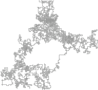
Figure 1: A square lattice random loop (left) and the corresponding outer boundary (right).

Note that the outer boundary is not a self-avoiding polygon, since it has cut vertices. The simulations suggest however that such vertices occur with zero density in the limit of infinite length of the outer boundary.

We considered the cases of the square lattice and the triangular lattice. The triangular lattice case was implemented on the computer using a square lattice with additional edges along the positive diagonal of each square. Due to piecewise linearity, the area $A$ of a loop $(v_{0},v_{1},\ldots,v_{N})$ is, on both lattices, given by

$$A=\sum_{i=0}^{N}(v_{i+1,x}-v_{i,x})\frac{v_{i+1,y}+v_{i,y}}{2},$$

where $v_{i,x}$ and $v_{i,y}$ denote the $x$-coordinate and $y$-coordinate of the vertex $v_{i}$, and $v_{N+1}=v_{0}$. It can thus be determined “on the fly” together with the construction of the outer boundary.

We generated random walks up to length $10^{5}$ on the square and triangular lattices, using the random number generator ran2.c [19]. For each lattice, we generated $10^{8}$ random walks. The size of the array was chosen such that the random walks did not reach the array boundaries. In our situation, an array of size $5000\times 5000$ was sufficient. For those random walks returning to their start point, we constructed the outer boundary and computed the values of the first ten area moments for perimeter up to $10^{3}$, i.e., we sampled $\mathbb{E}[Y^{k}_{m}]$ for $m<10^{3}$ and $k\leq 10$. Note that only even values of $m$ occur for the square lattice. For the data analysis, we rejected all values of $m$ with less than $10^{4}$ samples. Furthermore, we chose $m\geq 50$ in order to reduce finite size effects. This led to $50\leq m\leq 512$ for the square lattice and to $50\leq m\leq 401$ for the triangular lattice. The total number of loops used in the data analysis was $8.6\times 10^{6}$ for the square lattice and $11.6\times 10^{6}$ for the triangular lattice.

We first analysed the predicted power-law behaviour of the area moments (5)

$$\mathbb{E}[Y_{m}^{k}]\sim A_{k}m^{\alpha_{k}}\qquad(m\to\infty),$$ (6)

with $\alpha_{k}=3k/2$. Estimates of $\alpha_{k}$ were obtained by a least squares fit of the data to the assumed asymptotic form

$$\log(\mathbb{E}[Y_{m}^{k}])\sim\log A_{k}+\alpha_{k}\log m+\sum_{l=1}^{N}\frac{B_{k,l}}{m^{\beta_{k,l}}}\qquad(m\to\infty).$$ (7)

Since the exponents of the corrections to the asymptotic behaviour of (5) are not known, we chose $\beta_{k,l}=l$. This corresponds to analytic correction terms in (5). The results of a least squares fit with $N=3$ are shown in Table 1. The numbers in brackets give the statistical error of the fit in the last two digits. We found that differences in the estimates of $\alpha_{k}$ due to different choices of the exponents $\beta_{k,l}$ are an order in magnitude smaller than the statistical errors. This reflects the observation that the statistical fluctuations of the data points dominate effects due to different corrections to the asymptotic behaviour (6). The obtained values are consistent with the prediction $\alpha_{k}=3k/2$, which we employ in the following.

$k$	1	2	3	4	5
Square $\alpha_{k}$	1.522(41)	3.043(85)	4.56(14)	6.08(20)	7.60(27)
Triangular $\alpha_{k}$	1.508(81)	3.02(16)	4.53(24)	6.04(34)	7.56(45)

$k$	6	7	8	9	10
Square $\alpha_{k}$	9.12(36)	10.63(48)	12.14(62)	13.65(80)	15.1(10)
Triangular $\alpha_{k}$	9.08(58)	10.60(73)	12.11(90)	13.6(11)	15.2(14)

Table 1: Estimates of the exponents $\alpha_{k}$ of the area moments $\mathbb{E}[Y_{m}^{k}]$ on the square and triangular lattices. The numbers in brackets denote the statistical error of the fit in the last two digits.

We then tested our prediction for the area moment amplitudes. It follows from (5) that the ratios $A_{k}/A_{1}^{k}$ are independent of the constant $C$. In particular, we get

$$A_{2k}/A_{1}^{2k}=\frac{2^{6k-2}}{\pi^{k}}\frac{(3k-2)!}{(6k-3)!}\Omega_{2k},\qquad A_{2k+1}/A_{1}^{2k+1}=\frac{2}{\pi^{k}}\frac{1}{(3k)!}\Omega_{2k+1},$$ (8)

where the numbers $\Omega_{k}$ are the Airy constants defined in (2). We extrapolated the numbers $A_{k}/A_{1}^{k}$ by a least squares fit to $\mathbb{E}[Y_{m}^{k}]/\mathbb{E}[Y_{m}]^{k}\sim A_{k}/A_{1}^{k}+c_{k}/m+d_{k}/m^{2}$ as $m\to\infty$. A typical data plot is shown in Figure 2.

Figure 2: MC estimates of $\mathbb{E}[Y_{m}^{2}]/\mathbb{E}[Y_{m}]^{2}$ on the square lattice, plotted against $1/m$.

The corresponding results for the first ten amplitude ratios are given in Table 2, together with their predicted values. The numbers in brackets give the statistical error of the fit in the last two digits.

Amplitude	Airy distribution	Square MC	Triangular MC
$A_{2}/A_{1}^{2}$	1.06103296	1.0626(18)	1.0620(23)
$A_{3}/A_{1}^{3}$	1.19366208	1.1980(52)	1.1951(61)
$A_{4}/A_{1}^{4}$	1.42171312	1.430(13)	1.422(15)
$A_{5}/A_{1}^{5}$	1.78895216	1.801(28)	1.783(31)
$A_{6}/A_{1}^{6}$	2.37205758	2.387(59)	2.350(61)
$A_{7}/A_{1}^{7}$	3.30494239	3.32(12)	3.24(12)
$A_{8}/A_{1}^{8}$	4.82446133	4.83(25)	4.68(24)
$A_{9}/A_{1}^{9}$	7.35752352	7.32(52)	7.02(48)
$A_{10}/A_{1}^{10}$	11.6901282	11.5(11)	10.93(98)

Table 2: Comparison of amplitude ratios arising from the Airy distribution against MC estimates for the square and triangular lattice. The numbers in brackets denote the statistical error of the fit in the last two digits.

Finally, we estimated the constant $C$ in (5) using the first area moment $\mathbb{E}[Y_{m}]\sim C\sqrt{\pi}\,m^{3/2}$ as $m\to\infty$. A least squares fit to $\mathbb{E}[Y_{m}]/m^{3/2}$ with a polynomial of degree 4 in $1/m$ yields $C_{sq}=0.0910(11)$ for the square lattice and $C_{tr}=0.1262(29)$ for the triangular lattice.

4 Conclusion

Our numerical analysis supports the conjecture that the area of the outer boundary of planar random loops is Airy distributed, on both the square and triangular lattices. Since we expect this result to be universal, it would be interesting to check the appearance of the Airy distribution for boundaries of random walks on, for example, non-periodic tilings such as the Penrose tiling or the Ammann-Beenker tiling. Also, the question arises whether the Airy distribution can be found in other models of cluster boundaries with fractal dimension $4/3$. The outstanding question is whether our conjecture can be proved, possibly by using quantum gravity methods [4] or the probabilistic approach [2].

Appendix: Scaling functions and limit distributions

We explain how limit distributions are derived from the scaling function of a combinatorial model. We show, in particular, how the Airy distribution is derived from the scaling function of polygon models [20] such as staircase polygons or self-avoiding polygons. This relates the scaling function viewpoint employed in [13, 16, 15] to the present approach. In particular, it motivates formula (5).

For a polygon model on a given lattice, denote the number of polygons of (half-) perimeter $m$ and area $n$ by $p_{m,n}$. The perimeter and area generating function of the model is given by $G(x,q)=\sum_{m,n}p_{m,n}x^{m}q^{n}$. The function $G(x,1)=g_{0}(x)$ is called the perimeter generating function. Let $x_{c}$ denote the radius of convergence of the perimeter generating function. Typically [18], the factorial area moment generating functions $g_{k}(x)$ have the asymptotic behaviour

$$g_{k}(x)=\frac{(-1)^{k}}{k!}\left.\frac{\mbox{d}^{k}}{\mbox{d}q^{k}}G(x,q)\right|_{q=1}\sim\frac{f_{k}}{(x_{c}-x)^{\gamma_{k}}}\qquad(x\to x_{c}^{-}),$$ (9)

with critical amplitudes $f_{k}$ and critical exponents $\gamma_{k}$, where $\gamma_{k+1}>\gamma_{k}$. See [20, Ch. 7] for a proof that the functions $g_{k}(x)$ exist and are finite for polygon models. It is convenient to incorporate the numbers $f_{k}$ and $\gamma_{k}$ into the function [13, 18]

$$F(s)=\sum_{k=0}^{\infty}\frac{f_{k}}{s^{\gamma_{k}}}.$$ (10)

Typically, the function $F(s)$ describes scaling behaviour of the perimeter and area generating function about $(x,q)=(x_{c},1)$,

$$G^{(sing)}(x,q)\sim(1-q)^{\theta}F\left(\frac{x_{c}-x}{(1-q)^{\phi}}\right)\qquad(x,q)\to(x_{c}^{-},1^{-}),$$ (11)

with critical exponents $\theta$ and $\phi$. The function $F(s)$ is also called the scaling function. The form (11) is consistent with (9) if the exponents $\gamma_{k}$ are of the form $\gamma_{k}=(k-\theta)/\phi$. One should note that (11) has been proved only for a few examples including staircase polygons [21]. For typical polygon models such as staircase polygons and rooted self-avoiding polygons [13], the scaling function has the particular form [18, Eqn. 3.9]

$$F(s)=-4f_{1}\frac{\rm d}{{\rm d}s}\log\mbox{Ai}\left(\left(\frac{f_{0}}{4f_{1}}\right)^{2/3}s\right),$$ (12)

with critical exponents $\theta=1/3$ and $\phi=2/3$.

We now turn to a probabilistic description, see also [17]. Selecting polygons uniformly among the set of all polygons with perimeter $m$ defines a discrete random variable $X_{m}$ with probability distribution

$$\mathbb{P}(X_{m}=n)=\frac{p_{m,n}}{\sum_{n}p_{m,n}},$$ (13)

whose moments are given by

$$\mathbb{E}[X_{m}^{k}]=\frac{\sum_{n}n^{k}p_{m,n}}{\sum_{n}p_{m,n}}.$$ (14)

The numerator in (14) is related to the coefficients of the factorial moment generating functions (9) via

$$\frac{(-1)^{k}}{k!}\sum_{n}n^{k}p_{m,n}\sim\frac{(-1)^{k}}{k!}\sum_{n}(n)_{k}\,p_{m,n}=[x^{m}]g_{k}(x)\sim\frac{f_{k}}{x_{c}^{\gamma_{k}}\Gamma(\gamma_{k})}x_{c}^{-m}m^{\gamma_{k}-1}\qquad(m\to\infty),$$ (15)

where $(n)_{k}=n(n-1)\cdots(n-k+1)$, and $\Gamma(z)$ is the Gamma function. This relation can be used to characterise the leading asymptotic behaviour of the moments $\mathbb{E}[X_{m}^{k}]$ of the underlying distribution. Let us introduce distribution coefficients $\Phi_{k}$ defined by $f_{k}=-\frac{(-1)^{k}}{k!}2^{k}\Phi_{k}f_{1}^{k}f_{0}^{1-k}$. We obtain

$$\mathbb{E}[X_{m}^{k}]\sim-\frac{\Gamma(\gamma_{0})}{\Gamma(\gamma_{k})}\left(\left(\frac{m}{x_{c}}\right)^{1/\phi}\frac{2f_{1}}{f_{0}}\right)^{k}\Phi_{k}\qquad(m\to\infty).$$ (16)

Now introduce a normalised random variable ${\widetilde{X}}_{m}$ defined by

$${\widetilde{X}}_{m}=\frac{X_{m}}{\left(\frac{m}{x_{c}}\right)^{1/\phi}\frac{2f_{1}}{f_{0}}}.$$ (17)

The moments $\mathbb{E}[{\widetilde{X}}_{m}^{k}]$ of the normalised random variable ${\widetilde{X}}_{m}$ are then asymptotically given by

$$\mathbb{E}[{\widetilde{X}}_{m}^{k}]\sim-\frac{\Gamma(\gamma_{0})}{\Gamma(\gamma_{k})}\Phi_{k}\qquad(m\to\infty).$$ (18)

Note that (18) is independent of $x_{c}$ and asymptotically constant. In conjunction with (3), it follows that the particular scaling function (12) leads to the Airy distribution (1) in (18). Formula (5) is chosen in analogy with (16).

References

- [1] Smirnov S and Werner W 2001 Critical exponents for two-dimensional percolation Math. Res. Lett. 8 729–744; math.PR/0109120
- [2] Lawler G F Schramm O and Werner W 2001 The dimension of the planar Brownian frontier is 4/3 Math. Res. Lett. 8 13–23; math.PR/0010165
- [3] Mandelbrot B 1982 The Fractal Geometry of Nature (New York: Freeman)
- [4] Duplantier B 1998 Random walks and quantum gravity in two dimensions Phys. Rev. Lett. 81 5489–5492
- [5] Werner W 2003 Random planar curves and Schramm-Loewner evolutions preprint; math.PR/0303354
- [6] Cardy J and Ziff R 2003 Exact results for the universal area distribution of clusters in percolation, Ising and Potts models J. Stat. Phys. 110 1–33; cond-mat/0205404
- [7] Madras N and Slade G 1993 The Self-Avoiding Walk (Boston: Birkhäuser)
- [8] Lawler G F Schramm O and Werner W 2002 On the scaling limit of planar self-avoiding walk preprint; math.PR/0204277
- [9] Kennedy T 2001 Monte Carlo tests of SLE predictions for the 2D self-avoiding walk preprint; math.PR/0112246
- [10] Kennedy T 2002 Conformal invariance and Stochastic Loewner Evolution predictions for the 2D self-avoiding walk - Monte Carlo tests preprint; math.PR/0207231
- [11] Louchard G 1984 Kac’s formula, Lévy’s local time and Brownian excursion J. Appl. Prob. 21 479–499.
- [12] Flajolet P and Louchard G 2001 Analytic variations on the Airy distribution Algorithmica 31 361–377
- [13] Richard C Guttmann A J and Jensen I 2001 Scaling function and universal amplitude combinations for self-avoiding polygons J. Phys. A: Math. Gen. 34 L495–L501; cond-mat/0107329
- [14] Cardy J L 2001 Exact scaling functions for self-avoiding loops and branched polymers J. Phys. A: Math. Gen. 34 L665–L672; cond-mat/0107223
- [15] Jensen I 2003 A parallel algorithm for the enumeration of self-avoiding polygons on the square lattice J. Phys. A: Math. Gen. 36 5731–5745; cond-mat/0301468
- [16] Richard C Jensen I and Guttmann A J 2003 Scaling function for self-avoiding polygons in: Proceedings of the International Congress on Theoretical Physics TH2002, Paris (Supplement) eds Iagolnitzer D Rivasseau V and Zinn-Justin J (Basel: Birkhäuser) 267–277; cond-mat/0302513
- [17] Duchon P 1999 -grammars and wall polyominoes Ann. Comb. 3 311–321
- [18] Richard C 2002 Scaling behaviour of two-dimensional polygon models J. Stat. Phys. 108 459–493; cond-mat/0202339
- [19] Press W H Teukolsky S A Vetterling W T and Flannery B P 1992 Numerical Recipes in C (Cambridge: Cambridge University Press) http://www.nr.com
- [20] Janse van Rensburg E J 2000 The Statistical Mechanics of Interacting walks, Polygons, Animals and Vesicles New York: Oxford University Press
- [21] Prellberg T 1995 Uniform -series asymptotics for staircase polygons J. Phys. A: Math. Gen. 28 1289–1304