Chiral persistent currents and magnetic susceptibilities in the parafermion quantum Hall states in the second Landau level with Aharonov–Bohm flux

Abstract

Using the effective conformal field theory for the quantum Hall edge states we propose a compact and convenient scheme for the computation of the periods, amplitudes and temperature behavior of the chiral persistent currents and the magnetic susceptibilities in the mesoscopic disk version of the ${\mathbb{Z}}_{k}$ parafermion quantum Hall states in the second Landau level. Our numerical calculations show that the persistent currents are periodic in the Aharonov–Bohm flux with period exactly one flux quantum and have a diamagnetic nature. In the high-temperature regime their amplitudes decay exponentially with increasing the temperature and the corresponding exponents are universal characteristics of non-Fermi liquids. Our theoretical results for these exponents are in perfect agreement with those extracted from the numerical data and demonstrate that there is in general a non-trivial contribution coming from the neutral sector. We emphasize the crucial role of the non-holomorphic factors, first proposed by Cappelli and Zemba in the context of the conformal field theory partition functions for the quantum Hall states, which ensure the invariance of the annulus partition function under the Laughlin spectral flow.

I Introduction

According to a well-known but unpublished theorem due to Bloch Thouless (1998), the free energy of a conducting ring (or other non-simply connected conductor) is a periodic function of the magnetic flux through the ring with period one flux quantum $\phi_{0}=h/e=1$. The flux dependence of the free energy $F(T,\phi)=-k_{B}T\ln(Z(T,\phi))$, where $Z(T,\phi)$ is the partition function, gives rise to a non-dissipative equilibrium current

$$I=-\left(\frac{e}{h}\right)\frac{\partial F(T,\phi)}{\partial\phi},$$

flowing along the ring, called a persistent current, which has a universal amplitude and universal temperature dependence. Such currents have been experimentally observed in conducting mesoscopic rings Mailly et al. (1993), in which the circumference of the ring is smaller than the coherence length Geller (2001). Mesoscopic effects, such as the persistent currents and Aharonov–Bohm (AB) magnetization, offer an outstanding possibility for the experimental observation of certain implications of Quantum Mechanics. This has recently become a topical issue in the context of Quantum Computation Aharonov (1998). Another motivation for our interest in mesoscopic physics is that despite being equilibrium quantities the persistent currents may give important information about transport due to a recently emerging relation between the Thouless energy, diagonal conductivity and the persistent currentsAltland et al. (1996); Deo (1997). At the same time, these phenomena could help us understand the effects of electron–electron interaction on the strongly correlated electron systems Chakraborty and Pietiläinen (1994, 1995).

The fractional quantum Hall (FQH) effect provides an exciting possibility for an experimental realization of mesoscopic ringsGeller (2001); Geller and Loss (1997); Geller et al. (1996); Ino (1998). Due to the non-zero energy gap in the bulk, when the system is on a FQH plateau, the only delocalized states, which are able to carry electric current, live on the edge of the FQH sample. When this sample has the shape of a disk, its edge is a circular ring whose width is of the order of the magnetic length $l_{B}=\sqrt{\hbar/eB}$. For example, the edge states of the Laughlin FQH states gave the first observable realizations of the chiral Luttinger liquids Geller (2001), whose mesoscopic properties have been well-understood.

However, recent experiments Grayson et al. (1998) have shown that the Luttinger liquid theory is not relevant for more general filling factors such as those in the principle Jain series. Fortunately, there is a more general and promising classification scheme for the FQH states based on the conformal field theory (CFT). Within this scheme the universality classes of the FQH systems have been described by the effective field theories for the edge states in the (thermodynamic) scaling limit Fröhlich and Kerler (1991); Fröhlich et al. (1997, 2001). These turned out to be Chern–Simons topological field theories in $2+1$ dimensional space-time which are equivalent to unitary CFTs operating on the $1+1$ dimensional space-time border, provided the bulk excitations are suppressed by a finite energy gap.

Most of the computations of the persistent currents in FQH states for finite temperatures have been based so far on the Fermi/Luttinger liquid picture. The reason is that a more general approach to these quantities was missing. In this paper we are trying to bridge the gap between the general FQH classification scheme based on unitary CFT and the directly measurable quantities, such as the AB magnetization and magnetic susceptibility, which express the electro-magnetic properties of the mesoscopic FQH systems. To this end we shall use as a thermodynamical potential the complete chiral CFT partition function for the FQH edge states with AB flux and a special invariance condition, called the $V$ invariance, representing the Laughlin spectral flowLaughlin (1983); Cappelli and Zemba (1997) in the CFT context, which was introduced by Cappelli and Zemba Cappelli and Zemba (1997).

Typically the persistent currents in the FQH states contain large non-mesoscopic contributions Geller and Vignale (1995); Geller (2002), slowly varying with the magnetic field, coming from states which are deep below the Fermi level. These contributions cannot be described within the CFT framework which takes into account only states close to the Fermi energy and therefore the edge states effective CFT is relevant only for the computation of the (oscillating) mesoscopic part of the persistent currents, which is proportional to the AB magnetization. Fortunately, it is possible to measure directly the oscillating part of the persistent currents due to the DC Josephson effect in a 2-terminal superconducting ring, which is known as a Superconducting Quantum Interference Device (SQUID) Thouless (1998); Mailly et al. (1993). Perhaps, the persistent current and the AB magnetization are the only CFT-based prediction of electro-magnetic properties of the FQH systems that could be tested directly. As we shall see in Sect. IV, these currents are expected to be diamagnetic at very low temperature for any FQH state.

Although the FQH states do emerge in highly correlated electron systems it was confirmed both numerically Chakraborty and Pietiläinen (1994, 1995) and experimentally Mailly et al. (1993) that the electron–electron interaction does not change significantly the value of the persistent currents. On the contrary, it was found that the amplitude of the current is strongly reduced by impurities Chakraborty and Pietiläinen (1994, 1995), however, since the persistent currents for a disk FQH sample are chiral (for states without counter-propagating modes on the same edge) there should be no impurity backscattering, hence no amplitude reduction from weak disorder Geller and Loss (1997). Therefore, the temperature dependence of the persistent currents in mesoscopic FQH edges is expected to be universal. While the persistent currents naturally express the electric properties of the system, it turns out that their universal temperature dependence could also give important information about the neutral structure of the effective field theory for the edge states Geller et al. (1996); Ino (1998), and may be considered as an ideal tool for distinguishing between different FQH universality classes. As we shall demonstrate in Sect. IV and Sect. V the low- and high- temperature decays of the persistent current’s amplitudes crucially depend on the neutral properties of the edge states.

In 1999 the first several FQH states in the so called parafermionic (PF) hierarchy in the second Landau level with filling factors

$$\nu_{H}:=\frac{n_{H}}{d_{H}}=\frac{k}{k+2},$$ (1)

introduced by Read and Rezayi Read and Rezayi (1998) have been observed in an extremely high-mobility sample Pan et al. (1999) (for FQH states in the second Landau level one has to addRead and Rezayi (1998); Cappelli et al. (2001) $2$ to the filling factor in Eq. (1)). Originally the wave functions of the ground state and excited states of these novel FQH liquids have been obtained Read and Rezayi (1998) as conformal blocks of the well-known ${\mathbb{Z}}_{k}$ parafermions, however, in a subsequent work Cappelli et al. (2001) the effective CFT have been expressed as a diagonal affine coset within an abelian parent CFT (a multi-component Luttinger liquid). The latter approach allowed to find a much simpler expression for the wave functions as well as to interpret the non-abelian quasiparticles as a result of certain projection of neutral degrees of freedom.

In this paper we are going to illustrate the general CFT approach to the chiral persistent currents on the example of the parafermion FQH states in the second Landau level. Our main result is the observation that all mesoscopic quantities, such as the persistent current, AB magnetization and magnetic susceptibility, are periodic functions of the AB flux with period exactly one flux quantum $h/e$. Let us note that the Bloch theorem does not forbid fractional periods, such as $1/2$, $1/3$, $1/4$, etc., however, this is always a signal of spontaneous breaking of symmetries. Thus, our numerical results rule out this possibility for finite temperatures like it should be in view of the Mermin–WagnerMermin and Wagner (1966) and Coleman Coleman (1973) theorems.

We shall investigate the temperature dependence of the persistent currents much above some temperature scale $T_{0}=\hbar v_{F}/\pi k_{B}L$, where $v_{F}$ is the Fermi velocity on the edge and $L$ is the edge’s circumference, where the current’s amplitudes decay exponentially with increasing the temperature. The corresponding exponents are universal and can be used to characterize the universality classes of the FQH states. For example, for the Laughlin FQH states with $\nu_{H}=1/(2p+1)$, the amplitude of the persistent current decays according toGeller and Loss (1997); Georgiev (2003a)

$$I_{\max}^{\mathrm{Laugh}}(T)\mathop{\simeq}_{T\gg T_{0}}\ I_{0}\ \frac{T}{T_{0}}\ \exp\left(-\alpha\frac{T}{T_{0}}\right),\quad\alpha=\frac{1}{\nu_{H}}$$ (2)

(notice that the term $T/T_{0}$ is missing in Eq. (95) in Ref. Geller and Loss (1997) which is a misprint). For Fermi liquids $\alpha=1$ and any different value is the fingerprint of a non-Fermi liquid. A very interesting question in this context, which was one more motivation for our numerical calculations, is what would be the value of the universal exponent $\alpha$ for FQH states for which the numerator of $\nu_{H}$ is bigger than $1$? As we shall see in this paper, the answer to this question is not trivial and two obvious generalizations, namely $\alpha=\nu_{H}^{-1}$ and $\alpha=n_{H}d_{H}$ (see Eq. (1)), are inconsistent with the numerical data for the parafermion FQH states. Our result, Eq. (30), which is fairly instructive about the general pattern, shows that there is a non-trivial contribution from the neutral sector. To the best of my knowledge, this is the first generalization of this kind which is confirmed numerically.

The rest of this paper is organized as follows: in Sect. II we first describe the relation between the Cappelli–Zemba factors, the AB flux and the Laughlin spectral flow and then summarize the results from Ref. Cappelli et al. (2001) about the partition functions for the edge states of the parafermion FQH states for $k=2,3$ and $4$. In Sect. III we present the numerical calculations for the persistent currents and magnetic susceptibilities at fixed temperature, when the flux is varied within the range of one flux quantum, as well as for the temperature dependence of their amplitudes. In Sect. IV we derive the low-temperature asymptotics of the persistent currents and susceptibilities for these states and try to identify the possible mechanism for the amplitude reduction. In Sect. V the high-temperature asymptotics is computed with the help of the modular S-transformation which relates the low- and high-temperature regimes. Another mechanism for the temperature decay of the persistent currents is suggested for this regime. It is shown that both low- and high- temperature behaviors depend crucially on the neutral properties of the FQH system. Finally in Sect. VI we collect the arguments for our conclusion that the periods of the persistent currents in the parafermion FQH states is exactly one flux quantum.

II Chiral partition function for the FQH states with Aharonov–Bohm flux

II.1 Cappelli–Zemba factors and the Laughlin spectral flow

The partition function $Z(\tau,\zeta)$ for a disk FQH sample with a single edge, which we shall call the chiral partition function, computed within the effective CFT for the edge states is simply the sum of all non-equivalent chiral CFT charactersGeorgiev (2003b) $\chi_{\lambda}(\tau,\zeta)$

$$Z(\tau,\zeta) = \mathop{\mathrm{tr}}_{\ \ {\mathcal{H}}\ }q^{L_{0}-c/24}\,\mathrm{e}^{2\pi i\zeta J_{\mathrm{el}}}=\sum_{\lambda=1}^{N}\chi_{\lambda}(\tau,\zeta),\ \mathrm{where}$$

$$\chi_{\lambda}(\tau,\zeta) = \mathop{\mathrm{tr}}_{\ \ {\mathcal{H}}_{\lambda}\ }q^{L_{0}-c/24}\,\mathrm{e}^{2\pi i\zeta J_{\mathrm{el}}}\ \ \mathrm{and}\ \ {\mathcal{H}}=\mathop{\oplus}_{\lambda=1}^{N}{\mathcal{H}}_{\lambda}.$$ (3)

The number $N$ in Eqs. (II.1), called the topological orderWen (1995), (the number of topologically inequivalent quasiparticles with electric chargeFröhlich et al. (2001) $0\leq Q_{\mathrm{el}}<1$) is one of the most important characteristics of the FQH universality classes. The (Hilbert) space of the edge states ${\mathcal{H}}$, over which the trace in Eq. (II.1) is taken, is the direct sum of all independent (i.e., irreducible, topologically non-equivalent) representations ${\mathcal{H}}_{\lambda}$ of the chiral algebra (see the Introduction of Ref. Georgiev (2002) for a short description of the chiral algebra terminology in the FQH effect). The effective Hamiltonian for the edge states (in the thermodynamic limit) is essentially given by Cappelli and Zemba (1997)

$$H_{\mathrm{CFT}}=\hbar\frac{v_{F}}{R}\left(L_{0}-\frac{c}{24}\right),\quad L_{0}=\oint\frac{d\,z}{2\pi i}\ z\,T(z)$$ (4)

where $z=\exp[(v_{F}t-ix)/R]$, $x$ is the coordinate on the edge, $t$ is the imaginary time, $v_{F}$ is the Fermi velocity on the edge, $R$ is its radius, $L_{0}$ is the zero mode of the Virasoro stress tensor $T(z)$ and $c$ is the central charge of the latter Di Francesco et al. (1997). While it has become a wide-spread opinion that the CFT Hamiltonian (4) captures only the universal properties of realistic FQH systems and eventually could not give a physical description of the latter, it has been shown Cappelli et al. (1996) that the energy spectrum of the FQH edge excitations, with Coulomb and generic short-range interactions included, contain only logarithmic corrections to that derived from Eq. (4) which are subleading in the thermodynamic limit. Therefore, we believe that the CFT approach to the FQH effect could give more information about the structure of the Hilbert space of the low-laying excitationsCappelli et al. (1996), the energy spectrum of the FQH systems in the thermodynamic limit and even about the energy gap Georgiev (2002). In particular, it should not be a surprise that the CFT-based computations Ino (1998); Georgiev (2003a) of the persistent currents in the Laughlin FQH states give the same results as those based on the Luttinger liquid picture Geller and Loss (1997).

The electric charge operator $J_{\mathrm{el}}$ in Eq. (II.1), defined as the space integral of the charge density on the edge $J_{\mathrm{el}}(z)=\sqrt{\nu_{H}}J(z)$, proportional to the normalized $\widehat{u(1)}$ current $J(z)$ and has the following (short-distance) operator product expansion Di Francesco et al. (1997); Cappelli and Zemba (1997); Georgiev (2002)

$$J_{\mathrm{el}}=\oint\frac{d\,z}{2\pi i}\ J_{\mathrm{el}}(z),\quad J_{\mathrm{el}}(z)J_{\mathrm{el}}(w)\simeq\frac{\nu_{H}}{(z-w)^{2}}.$$

The modular parameters $q$ and $\zeta$ entering Eq. (II.1) are generically restricted for an annulus sample by the convergence conditions

$$q=\mathrm{e}^{2\pi i\tau},\quad 0<\mathrm{Im}\,\tau\sim\frac{1}{k_{B}T},\quad\zeta\in{\mathbb{C}}$$

and their real and imaginary parts are related to the inverse temperature, chemical potential and Hall voltage Cappelli and Zemba (1997). For the disk FQH sample, however, both $\tau$ and $\zeta$ have to be purely imaginary in order for the partition function Eq. (II.1) be real. Before we establish the exact relation between the modular parameters and the physical quantities for the disk FQH sample we need to recall some of the general properties of the corresponding CFTs. The characters $\chi_{\lambda}(\tau,\zeta)$ in Eq. (II.1), like those in any rational CFT, belong to a finite dimensional representation of the fermionic subgroup of the modular group Cappelli et al. (2001); Fröhlich et al. (2001); Cappelli and Zemba (1997) $PSL(2,{\mathbb{Z}})$. However, in the FQH context there are two more conditions to be satisfied Cappelli and Zemba (1997): the annulus partition function, which is a bilinear combination of the characters $\chi_{\lambda}(\tau,\zeta)$ and their complex conjugates, must be also invariant under the $U$ and $V$ transformations of the modular parameters Cappelli and Zemba (1997). The first one simply shifts the parameter $\zeta$, i.e., $U:\ \zeta\to\zeta+1$ and the second acts as follows

$$V:\ \zeta\to\zeta+\tau.$$ (5)

It is remarkable that the $V$ transformation (5) exactly represents the Laughlin spectral flow Laughlin (1983); Cappelli and Zemba (1997) in the CFT context, i.e., the mapping between orbitals, corresponding to increasing the orbital momentum by 1 (in the Laughlin FQH states), after adiabatically threading the sample with one quantum of AB flux. As a result of this flow a fractional amount of electron charge is transferred between the edges of the annulus, which is the basic mechanism inducing the Hall current.

Adding AB flux in the FQH system naturally introducesGeorgiev (2003b) twisted boundary conditions for the field operators of the electron and the quasiparticles and also modifies the Hamiltonian (4). The ultimate effect of this twistingGeorgiev and Todorov (1998) on the partition function is that the modular parameter $\zeta$ is shifted Georgiev (2003b) with an amount proportional to the modular parameter $\tau$ and the coefficient of proportionality has to be identified with the AB flux threading the surface of the FQH sample. This coefficient can be computed through the phase that the electron operator accumulates when traveling along the FQH edge encircling the AB flux $\phi$. In other words, within the rational CFT framework, the arbitrary flux ($\phi$) threading procedure is represented by the following transformation Georgiev (2003a, b)

$$\zeta\to\zeta+\phi\tau,\quad\phi\in{\mathbb{R}}.$$ (6)

This generalization of the $V$ transformation (5) is obviously consistent with the interpretation of the latter as the Laughlin spectral flow. More intuitively speaking, since the $V$ transformation, Eq. (5), was originally interpreted as increasing the AB flux by one unit, the transformation (6) should mean increasing the flux by the value $\phi$ (in units $\phi_{0}$). Note that Eq. (6) was used to compute the chiral persistent currents in the Laughlin FQH states reproducing the well-known result Geller and Loss (1997), see Appendix B in Ref. Georgiev (2003a).

We shall set $\zeta=0$ in Eq. (6), which corresponds to zero magnetic field (measured with respect to the uniform background magnetic field). Taking into account the interpretation of Eq. (6) and choosing the conventional temperature unit $T_{0}$ from Ref. Geller and Loss (1997) we make the following identification of the modular parameters in the context of a disk FQH sample threaded by AB flux $\phi$

$$\tau=i\pi\frac{T_{0}}{T},\quad\zeta=\phi\tau,\quad T_{0}=\frac{\hbar v_{F}}{\pi k_{B}L},\quad\phi\in{\mathbb{R}}.$$ (7)

In the above equation $T$ is the absolute temperature, $L=2\pi R$ is the circumference of the edge, $k_{B}$ the Boltzmann constant and $\phi$ the magnetic flux threading the FQH disk sample.

The important observation Cappelli and Zemba (1997) of Cappelli and Zemba is that the CFT partition function for the annulus sample is not $V$-invariant alone Cappelli and Zemba (1997) since the CFT characters $\chi_{\lambda}$ in Eq. (II.1) change their absolute values after the transformation (5). In order to preserve the norm of the characters $\chi_{\lambda}$, hence restore their $V$-covariance, these authors introduce special non-holomorphic exponential factors

$$\exp\left(-{\pi}\nu_{H}\frac{\left(\mathrm{Im}\,\zeta\right)^{2}}{\mathrm{Im}\,\tau}\right),$$ (8)

multiplying the characters $\chi_{\lambda}(\tau,\zeta)$ in Eq. (II.1), which we shall call the Cappelli–Zemba (CZ) factors. In the same way the total chiral partition function $Z(\tau,\zeta)$ in Eq. (II.1) becomes $V$-invariant only after multiplying the characters with the CZ factors (8). One consequence of the $V$-invariance condition is that one has to include all twisted sectors which are connected by the action of the spectral flow Eq. (5). This restricts the chiral partition function for the disk FQH sample to have the “diagonal” form like in Eq. (II.1). The physical interpretation of the multiplication with the CZ factors (8) is adding constant (capacitive) energy to both edges which makes the ground state energy independentCappelli and Zemba (1997) of the edge potential $V_{0}$. In the next sections we are going to show that the CZ factors play a fundamental role in the equilibrium thermodynamic phenomena, such as the persistent currents and AB magnetization. We believe that they could also be crucial in various transport processes.

II.2 Partition function for the ${\mathbb{Z}}_{k}$ parafermion FQH states

The CFT for the ${\mathbb{Z}}_{k}$ parafermions, which is denoted by Cappelli et al. (2001); Georgiev (2002)

$$\left(\widehat{u(1)}\oplus\mathrm{PF}_{k}\right)^{{\mathbb{Z}}_{k}},\quad\mathrm{PF}_{k}=\frac{\widehat{su(k)}_{1}\oplus\widehat{su(k)}_{1}}{\widehat{su(k)}_{2}}$$ (9)

contains a $u(1)$ factor describing the charge/flux degrees of freedom and a neutral parafermionic factor which is realized as a diagonal affine coset Cappelli et al. (2001). Both factors are subjected to a ${\mathbb{Z}}_{k}$ selection rule called the pairing ruleCappelli et al. (2001), which states that an excitation

$$:\mathrm{e}^{i\frac{\lambda}{\sqrt{k(k+2)}}\varphi(z)}:\otimes\ \Phi(z)$$

of the $\mathrm{PF}_{k}$ model with labels $(\lambda,\Phi)$, where $\varphi$ is the $u(1)$ chiral boson, $\lambda$ is the corresponding $u(1)$ charge label and $\Phi$ is a parafermion (primary) field Cappelli et al. (2001); Di Francesco et al. (1997), is legitimate only if

$$P\left[\Phi\right]\equiv\lambda\ \ \mathrm{mod}\ \ k,$$

with $P$ being the parafermion ${\mathbb{Z}}_{k}$ charge. The independent characters $\chi_{l,\rho}$ of the chiral CFT (whose number gives the topological order) for the parafermion FQH states in the second Landau level Cappelli et al. (2001) are labeled by two integer numbers $l\ \mathrm{mod}\ k+2$ (symmetric around $l=0$) and $\rho=0,\ldots,k-1$ with the restriction $\rho\geq l-\rho\ \mathrm{mod}\ k$

$$\chi_{l,\rho}(\tau,\zeta)=\sum_{s=0}^{k-1}K_{l+s(k+2)}(\tau,k\zeta;k(k+2))\mathrm{ch}\left(\underline{\Lambda}_{l-\rho+s}+\underline{\Lambda}_{\rho+s}\right)(\tau)$$ (10)

and the complete chiral partition function is defined as

$$Z_{k}(\tau,\zeta)=\mathrm{e}^{-{\pi}\nu_{H}\frac{\left(\mathrm{Im}\,\zeta\right)^{2}}{\mathrm{Im}\,\tau}}\sum_{l\ \mathrm{mod}\ k+2}\quad\sum_{\rho\geq l-\rho\ \mathrm{mod}\ k}\chi_{l,\rho}(\tau,\zeta),$$ (11)

where we have written the CZ factors (8) explicitly. The rational torus partition functions Di Francesco et al. (1997) $K_{l}$ represent the contribution of the charged sector

$$K_{l}(\tau,\zeta;m)=\frac{1}{\eta(\tau)}\sum_{n\in{\mathbb{Z}}}q^{\frac{m}{2}\left(n+\frac{l}{m}\right)^{2}}\mathrm{e}^{2\pi i\zeta\left(n+\frac{l}{m}\right)},$$ (12)

where $\eta$ is the Dedekind function Di Francesco et al. (1997)

$$\eta(\tau)=q^{\frac{1}{24}}\prod_{n=1}^{\infty}\left(1-q^{n}\right),$$ (13)

while the neutral characters $\mathrm{ch}(\underline{\Lambda}_{\mu}+\underline{\Lambda}_{\rho})$ which are labeledCappelli et al. (2001) by the $\widehat{su(k)_{2}}$ weights $\underline{\Lambda}_{\mu}+\underline{\Lambda}_{\rho}$ with $0\leq\mu\leq\rho\leq k-1$, are expressed in terms of the so called universal chiral partition functions Cappelli et al. (2001) $\mathrm{ch}^{Q}_{\sigma}$ with the identification $Q=\rho$, $\sigma=\rho-\mu$

$$\mathrm{ch}^{Q}_{\sigma}(\tau)=q^{\Delta_{\sigma}-\frac{c_{\mathrm{PF}}}{24}}\sum_{\mathop{n_{1},n_{2},\ldots,n_{k-1}=0}\limits_{[\underline{n}]\equiv Q\ \mathrm{mod}\ k}}^{\infty}\frac{q^{\underline{n}\cdot C^{-1}\cdot(\underline{n}-\underline{\Lambda}_{\sigma})}}{(q)_{n_{1}}\cdots(q)_{n_{k-1}}},\quad Q\geq\sigma.$$ (14)

In the above equation, $\underline{n}=(n_{1},n_{2},\ldots,n_{k-1})$ is a $k-1$ component vector with non-negative entries, $[\underline{n}]=\sum\limits_{i=0}^{k-1}i\,n_{i}$ is its $k$-ality,

$$\Delta_{\sigma}=\Delta^{\mathrm{PF}}\left(\underline{\Lambda}_{0}+\underline{\Lambda}_{\sigma}\right)=\frac{\sigma(k-\sigma)}{2k(k+2)}$$ (15)

is the CFT dimension of the $\mathrm{PF}_{k}$ primary field labeled byCappelli et al. (2001) $\underline{\Lambda}_{0}+\underline{\Lambda}_{\sigma}$, $c_{\mathrm{PF}}=\frac{2(k-1)}{k+2}$ is the parafermion central charge, $(q)_{n}=\prod\limits_{j=1}^{n}(1-q^{j})$ and $C^{-1}$ is the inverse of the $su(k)$ Cartan matrix.

In order to compute the partition functions with AB flux, we have to apply the flux transformation (6) to the partition function (IV). To this end we shall use the following important property of the $K$-functions

$$\mathrm{e}^{-{\pi}\nu_{H}\frac{\left(\mathrm{Im}\,(\zeta+\phi\tau)\right)^{2}}{\mathrm{Im}\,\tau}}K_{l}(\tau,n_{H}(\zeta+\phi\tau);n_{H}d_{H}))=$$

$$=\mathrm{e}^{-{\pi}\nu_{H}\frac{\left(\mathrm{Im}\,\zeta\right)^{2}}{\mathrm{Im}\,\tau}}K_{l+n_{H}\phi}(\tau,n_{H}\zeta;n_{H}d_{H})$$ (16)

applied for $\zeta=0$.

III Persistent currents and magnetic susceptibilities

The equilibrium thermodynamic chiral persistent current in the disk FQH system can be computed directly from the CFT partition function (II.1) as follows

$$I(T,\phi)=\left(\frac{e}{h}\right)k_{B}T\frac{\partial}{\partial\phi}\ln Z(\tau,\phi\tau),$$ (17)

where the temperature $T$ and the AB flux $\phi$ are related to the modular parameters $\tau$ and $\zeta$ according to Eq. (7). More explicit formulas for the chiral partition functions (11) and (10) for the parafermion FQH states, before and after threading the sample with arbitrary AB flux, can be found in Ref. Georgiev (2003a, b).

We have computed numerically the persistent currents using the definition Eq. (17) and the explicit formulas Eqs. (11), (10), (12) and (14) for the characters of the parafermion FQH states. All computations have been performed with unlimited number of terms for the partition functions (12) and finite number ($10^{k}$, with $k=2,3$ and $4$ respectively) of terms for the partition functions (14). The plots of the persistent currents profiles in the $\mathrm{PF}_{k}$ states with $k=2$, $3$ and $4$ and AB flux in the range $-1/2\leq\phi\leq 1/2$ for temperature $T/T_{0}=0.1$ are given on Fig. 1.

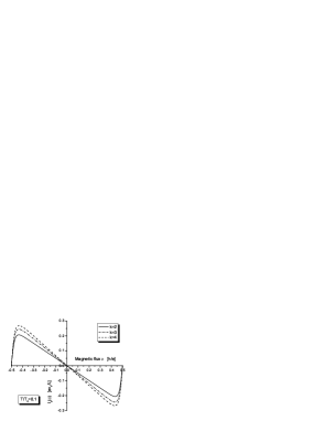
Figure 1: Persistent currents in the $k=2,3$ and $4$ parafermion FQH states, as functions of the magnetic flux within one period, computed numerically for $T/T_{0}=0.1$. The flux is measured in units $h/e$ and the current’s unit is $ev_{F}/L$. The period is 1 flux quantum for all states and the amplitudes are $I_{2}^{\max}=0.207$, $I_{3}^{\max}=0.245$ and $I_{4}^{\max}=0.268$.

According to the discussion in Sect. II.1, the partition function (11) constructed for the $\mathrm{PF}_{k}$ states must be invariant under the $V$ transformation Eq. (5), which implies that the corresponding chiral persistent current should be periodic in $\phi$ with period at most $1$. The plots in Fig. 1, indicate that all currents are periodic in $\phi$ with a period exactly one quantum of flux ($h/e$). We do not see anomalous oscillations with fractional flux periodicity of the persistent currents Ino (1998, 2000); Kiryu (2002) in the $k=2,3,4$ $\mathrm{PF}_{k}$ states for all temperatures $0.03\leq T/T_{0}\leq 14$ that we could access numerically. This is in perfect agreement with the Bloch theorem, known also as the Byers–Yang theorem Byers and Yang (1961) in the context of superconductors. Notice that the persistent currents for the Read–Rezayi FQH states have been shown in Ref. Kiryu (2002) to have anomalous oscillations for $M=0$ with periods smaller than $1$, however we argue that this case is physically irrelevant and has only been used in Ref. Read and Rezayi (1998) as a technical tool for investigating the wave functions for the $\mathrm{PF}_{k}$ states. One of the objectives of this paper was to show that the periods of the persistent currents for the $\mathrm{PF}_{k}$ states are exactly $1$ for all non-zero temperatures.

It is more realistic to consider the edge of a FQH disk sample as a very thin ring (with inner radius $R_{\mathrm{in}}$ and outer one $R_{\mathrm{out}}$) rather than just a circle, in which case $R$ is the average radius of the ring $R=(R_{\mathrm{in}}+R_{\mathrm{out}})/2$. Under the assumption that the width $w=R_{\mathrm{out}}-R_{\mathrm{in}}$ of the ring and the thickness $d$ of the physical 2-dimensional electron layer are much smaller than the ring’s circumference $L$, the magnetization of the FQH ring, like all thermodynamic quantities, can be expressed as a function of the magnetic flux (not of the magnetic field alone), and becomes simply proportional to the persistent current, i.e.,

$$M(T,\phi)=-\frac{1}{\mathrm{Vol}}\frac{\partial F(T,\phi)}{\partial B}=\frac{L}{4\pi wd}\ I(T,\phi),$$

where $\mathrm{Vol}=2\pi Rwd$ is the volume of the physical mesoscopic ring (with finite $w$ and $d$) and we have used $\partial/\partial B=\pi R^{2}\phi_{0}^{-1}\,\partial/\partial\phi$. Furthermore, the (isothermal) magnetic susceptibility is proportional to the derivative of the persistent current with respect to the flux

$$\kappa=\left.\frac{\partial M}{\partial H}\right|_{H=0}=\mu_{0}\frac{e}{h}\pi R^{2}\left.\frac{\partial M}{\partial\phi}\right|_{\phi=0}.$$ (18)

The magnetic susceptibilities for the parafermion FQH states with $k=2,3$ and $4$ have also been computed numerically and they also show periodicity with the flux with a period of one flux quantum exactly for all temperatures $0.03\leq T/T_{0}\leq 14$. The plots of the susceptibilities for temperature $T/T_{0}=0.1$ as functions of the flux within the range $0\leq\phi\leq 1$ are given on Fig. 2. We have chosen a different flux range in Fig. 2 in order to show the entire pick at $\phi=1/2$.

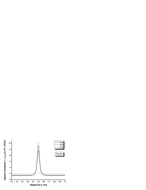
Figure 2: Magnetic susceptibilities in the $k=2,3$ and $4$ parafermion FQH states, as functions of the magnetic flux within one period, computed numerically for $T/T_{0}=0.1$. The flux is measured in units $h/e$ and the susceptibility unit is $v_{F}\frac{\mu_{0}}{4\pi}\frac{e^{2}}{h}\frac{\pi R^{2}}{wd}$, where $w$ and $d$ are respectively the finite width of the ring and the finite thickness of the 2 dimensional electron layer. The period is 1 flux quantum for all states.

The amplitudes of the persistent currents in the parafermion FQH states with $k=2$, $3$ and $4$, according to our computations, decay exponentially with temperature, as shown in Fig. 3.

Figure 3: Temperature decay of the persistent current’s amplitudes in the $k=2,3$ and $4$ parafermion FQH states (without the contribution from the two $\nu=1$ Landau levels with opposite spins) computed numerically in units $ev_{F}/L$, for temperatures measured in units of $T_{0}$. The zero temperature amplitudes in these units are $\nu_{k}/2$, i.e., $1/4,3/10$ and $1/3$ respectively.

Notice that, in order to compute these amplitudes we first analytically differentiate the logarithm of the partition function (11) with respect to $\phi$, according to Eq. (17), to get the persistent current $I(T,\phi)$, then differentiate analytically again with respect to $\phi$ and finally solve numerically $\partial I(T,\phi)/\partial\phi=0$ in the interval $-1/2<\phi<0$ to find the position of the maximum. The positions $\phi_{\max}$ of the maximums of the persistent currents, for $k=2$, $3$ and $4$ respectively, have been also plotted as functions of temperature on Fig. 7 and a more detailed discussion of this issue will be given in Sect. VI. The same three curves of Fig. 3, however within the full computational range of temperatures $0.03\leq T/T_{0}\leq 14$, have been also plotted in a (semi-) logarithmic plot on Fig. 6; the plots on Fig. 6 look almost linear, which means almost exponential decays for the amplitudes themselves. Each of the three curves on Fig. 6 contains 147 points and each point would need about 280 seconds (on average) to compute using MAPLE-8 on a 2 GHz class PC.

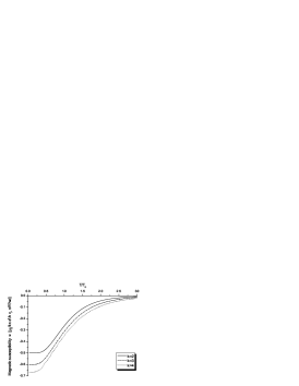
Figure 4: Temperature decay of the (zero-field) magnetic susceptibility in the $k=2,3$ and $4$ parafermion FQH states computed numerically in dimensionless units $v_{F}\frac{\mu_{0}}{4\pi}\frac{e^{2}}{h}\frac{\pi R^{2}}{wd}$, where $w$ and $d$ are respectively the finite width and thickness of a realistic 2D electron layer. The zero temperature susceptibilities in these units are exactly $-\nu_{k}$, i.e., $-1/2$, $-3/5$ and $-2/3$ respectively.

The magnetic susceptibilities (18) also decay very fast with temperature as shown on Fig. 4, for the $k=2$, $3$ and $4$ $\mathrm{PF}_{k}$ states. Moreover, since the susceptibility is a derivative of the persistent current, its temperature behavior determines the decay-type of the amplitude of the persistent current. It could be seen from Fig. 4 that there are two different temperature regimes in which the persistent currents’ amplitudes decay in different ways. Note that the function $\kappa(T)$ has an inflection point close to $T_{0}$ which can be interpreted as the crossover temperature between the two regimes. As we shall see in more detail in Sects. IV and V, there are indeed two different mechanisms for the temperature decay of the amplitude (cf. Ref. Mailly et al. (1993)). The first one, for $T\ll T_{0}$ is due to mixing of contribution of levels in an energy interval $k_{B}T$ which reduces the current since adjacent levels give opposite contributions Mailly et al. (1993). The energy scale for this mixing is set Mailly et al. (1993) by the energy gap. The second mechanism, which is essential for the current at temperatures higher than $T_{0}$, is a thermal smearing due to the reduction of the phase coherence length Mailly et al. (1993) $L_{\varphi}$ which makes the current vanish exponentially in $L/L_{\varphi}$. A more detailed discussion of this point will be given in Sect. V.

IV Low-temperature regime: $T\ll T_{0}$

In this Section we are going to find analytic expressions for the persistent current’s amplitudes and magnetic susceptibilities for the $\mathrm{PF}_{k}$ states in the limit $T\to 0$. Our low-temperature analysis would be valid for a class of FQH states which is larger than the parafermion states in the second Landau level. It would be based on the natural assumption that the CFT dimension of the fundamental quasihole is the minimal one allowed in the CFT, which is of course fulfilled in the $\mathrm{PF}_{k}$ states Cappelli et al. (2001); Georgiev (2002).

The low-temperature limit $T\to 0$ corresponds to the trivial limit $q\to 0$. Therefore we can keep only the first terms in the disk partition function (11) which, under the above mentioned assumption, come from the vacuum character and from those with the minimal non-trivial CFT dimension, i.e., from the sectors containing one quasiparticle (qp) or one quasihole (qh) so that

$$Z(\tau,\zeta)\mathop{\simeq}\limits_{\ T\ll T_{0}\ }\mathrm{e}^{-{\pi}\nu_{H}\frac{\left(\mathrm{Im}\,\zeta\right)^{2}}{\mathrm{Im}\,\tau}}\Bigl{(}K_{0}(\tau,n_{H}\zeta;n_{H}d_{H})\mathrm{ch}_{0}(\tau)+$$

$$K_{1}(\tau,n_{H}\zeta;n_{H}d_{H})\mathrm{ch}_{\mathrm{qh}}(\tau)+K_{-1}(\tau,n_{H}\zeta;n_{H}d_{H})\mathrm{ch}_{\mathrm{qp}}(\tau)\Bigr{)},\quad$$ (19)

where $\nu_{H}$, $n_{H}$ and $d_{H}$ are defined in Eq. (1) and the exponent in front of the parentheses is the CZ factor (8). Here we have denoted by $\mathrm{ch}_{\mathrm{qh}}=\mathrm{ch}(\underline{\Lambda}_{0}+\underline{\Lambda}_{1})$ and $\mathrm{ch}_{\mathrm{qp}}=\mathrm{ch}(\underline{\Lambda}_{0}+\underline{\Lambda}_{k-1})$ the coset characters corresponding to the neutral components of the quasiparticle and quasihole in the $\mathrm{PF}_{k}$ states.

Since, in order to compute the persistent current, we intend to differentiate with respect to $\phi$ according to Eq. (17)), we shall skip the $\phi$-independent factors containing the $\eta$-function and the central charge, which after taking the logarithm will give rise to additive flux-independent terms that will drop out after differentiation. Applying Eq. (II.2) in order to incorporate the AB flux and keeping only the first terms in Eq. (IV) we can write

$$Z(T,\phi)\mathop{\simeq}\limits_{\ T\ll T_{0}\ }q^{\frac{\nu_{H}}{2}\phi^{2}}\left\{1+q^{\Delta_{\mathrm{qh}}}\left(q^{Q_{\mathrm{qh}}\phi}+q^{-Q_{\mathrm{qh}}\phi}\right)\right\}=$$

$$=\mathrm{e}^{-\pi^{2}\frac{T_{0}}{T}\nu_{H}\phi^{2}}\left\{1+2\mathrm{e}^{-\frac{\widetilde{\varepsilon}_{\mathrm{qh}}}{k_{B}T}}\cosh\left(2\pi^{2}\frac{T_{0}}{T}Q_{\mathrm{qh}}\phi\right)\right\}$$ (20)

where

$$\widetilde{\varepsilon}_{\mathrm{qh}}=2\pi^{2}k_{B}T_{0}\Delta_{\mathrm{qh}},\quad\Delta_{\mathrm{qh}}=\frac{1}{2n_{H}d_{H}}+\Delta^{(0)}_{\mathrm{qh}},\quad Q_{\mathrm{qh}}=\frac{1}{k+2}.$$ (21)

In the above equation $\widetilde{\varepsilon}_{\mathrm{qh}}$ is the effective proper quasihole energy Morf and Halperin (1986); Geller and Loss (1997) (defined at fixed density), $\Delta_{\mathrm{qh}}$ is the total CFT dimension of the quasihole (with $\Delta^{(0)}_{\mathrm{qh}}$ being its neutral component) and $Q_{\mathrm{qh}}$ is the quasihole’s electric charge. The neutral CFT dimension $\Delta^{(0)}_{\mathrm{qh}}=(k-1)/(2k(k+2))$ of the quasihole for the $\mathrm{PF}_{k}$ states is obtained from EQ. (15) for $\sigma=1$. In the derivation of Eq. (IV) we have kept only the leading terms in the (neutral) coset characters $\mathrm{ch}_{0}(\tau)\simeq q^{0}$, $\mathrm{ch}_{\mathrm{qp}}(\tau)=\mathrm{ch}_{\mathrm{qh}}(\tau)\simeq q^{\Delta^{(0)}_{\mathrm{qh}}}$ for $q\to 0$ (again dropping the central charge term). Notice that the partition function (IV) is finite in this approximation Georgiev (2003b).

Next, we take the logarithm of Eq. (IV) and differentiate with respect to $\phi$ like in Eq. (17) to get the following expression for the persistent current for $|\phi|<1/2$

$$I(T,\phi)\ \mathop{\simeq}_{T\ll T_{0}}\ \frac{ev_{F}}{L}\left\{-\nu_{H}\phi+2Q_{\mathrm{qh}}\mathrm{e}^{-\frac{\widetilde{\varepsilon}_{\mathrm{qh}}}{k_{B}T}}\sinh\left(2\pi^{2}\frac{T_{0}}{T}Q_{\mathrm{qh}}\phi\right)\right\}.$$ (22)

IV.1 The persistent current’s amplitude for $T=0$

For $T=0$ the second term in the curly brackets in Eq. (22) vanishes expressing the fact that for zero temperature the free energy is determined by the ground state energy. Then the persistent current is a linear function of the flux

$$I(0,\phi)=-\nu_{H}\frac{ev_{F}}{L}\,\phi\quad\mathrm{for}\quad-\frac{1}{2}<\phi<\frac{1}{2}$$ (23)

and riches its maximum

$$I_{\max}=\frac{1}{2}\,\nu_{H}\,\frac{ev_{F}}{L}\quad\mathrm{for}\ T=0.$$

at $\phi=-1/2$. By periodicity, the current Eq. (23) could be continued to any value of the magnetic flux, which gives rise to the so called saw-tooth curve. The peak-to-peak value of the amplitude $ev_{F}/L$ for the mesoscopic sample of Ref. Mailly et al. (1993), for which $v_{F}\simeq 2.6\times 10^{5}$ m/s and $R\simeq 2.7\mu$m, is approximately $5$ nA.

The zero-field magnetic susceptibility (see Eq. (28) below) at zero temperature

$$\kappa(0)=-\nu_{H}\frac{\mu_{0}}{4\pi}\left(\frac{\pi R^{2}}{wd}\right)\frac{e^{2}}{h}v_{F},\quad w\ll R,\quad d\ll R$$ (24)

has absolute value of the order of $10^{-4}$ for the sample of Ref. Mailly et al. (1993).

Remark 1. The CZ factors (8) completely determine the zero-temperature behavior of the FQH system. In particular, they modify the ground state energy in presence of AB flux and therefore fix the zero-temperature behavior of the persistent current and magnetic susceptibilities.

We stress that Eq. (23) and Eq. (24) are derived entirely from the CZ factors and are therefore valid for all FQH states. They clearly show that the persistent currents in mesoscopic FQH edges are diamagnetic with respect to the AB flux at zero temperature. Our analysis for $T>0$ showed that the persistent currents in the parafermion FQH states remain diamagnetic for all numerically accessible temperatures $0.03\leq T/T_{0}\leq 14$, as illustrated on Fig. (1), Fig. (2) and Fig. (4). A similar phenomenon has been recently observed in a series of experiments with small numbers of metallic mesoscopic rings Deblock et al. (2002). A natural explanation of this result could be given by the Lenz rule for the Faraday induction: for polarized FQH states, where the magnetic degrees of freedom are frozen by the huge background magnetic field corresponding to a FQH plateau, the only response of the FQH system to the change in the flux is the magnetization persistent current, which creates magnetic field that is always opposite to the direction of the changes of the magnetic field that have created the current. On the other hand, the magnetic flux $\phi$ entering Eq. (7) is actually the difference between the total magnetic flux and that of the background magnetic field. Since the SQUID detectors measure exactly the oscillating part of the persistent current, when the flux $\phi$ is changed adiabatically, we expect that its magnetization should always be opposite to the direction of the changes of the flux. This may explain why the derivative of the persistent current is negative at $\phi=0$. In FQH states that are not completely polarized an eventual paramagnetic component could be dominant.

Remark 2. In principle the the persistent currents in the FQH states are paramagnetic for even parity and diamagnetic for odd parity of the number of electrons in the mesoscopic ring Loss (1992); Loss and Goldbart (1991); Kim et al. (2002). However, the parity of the electron number is not well-defined in the experimental setup of Ref. Mailly et al. (1993) so that one has to average over the electron parity. For example the average of the two currents in Eq. (14) in Ref. Kim et al. (2002) gives $1/2\,ev_{F}/L$ which coincides with the CFT prediction for the persistent currents in the thermodynamic limit.

Another interesting analogy can be made with the amplitude of the current (23). It is known Altland et al. (1996) that the zero temperature of the (disorder and sample averaged) persistent current for ballistic systems is proportional to the Thouless energy

$$|I(\phi)|=\frac{e}{h}E_{T}\phi,\quad\mathrm{for}\quad T=0$$

and $\phi$ measured in units of $\phi_{0}$. On the other hand the ratio of the Thouless energy and the level spacing $\Delta=\hbar\,2\pi v_{F}/L$, which is known as the Thouless number $g$, gives the dimensionless conductance. In our case this number coincides with the dimensionless Hall conductance

$$E_{T}=\nu_{H}\hbar\,\frac{2\pi v_{F}}{L},\quad g=\frac{E_{T}}{\Delta}=\nu_{H}.$$

IV.2 The persistent current’s amplitudes for $T>0$

According to Theorem 3 in Ref. Byers and Yang (1961) the partition function of the system should be an even periodic function of the flux $\phi$ with period $1$. Therefore the persistent current (17) must be an odd function with period $1$ so that it would be enough to consider the half interval $-1/2<\phi<0$ and continue it as an odd function $I(\phi)=-I(-\phi)$. Writing the $\sinh$ in Eq. (22) into its exponential form and ignoring $\exp(2\pi^{2}T_{0}Q_{\mathrm{qh}}\phi/T)$ which vanishes in the limit $T\to 0$ since $\phi$ is negative, we get

$$I(T,\phi)\ \mathop{\simeq}_{T\ll T_{0}}\ \frac{ev_{F}}{L}\left\{-\nu_{H}\phi-Q_{\mathrm{qh}}\mathrm{e}^{-\frac{\widetilde{\varepsilon}_{\mathrm{qh}}}{k_{B}T}}\mathrm{e}^{-2\pi^{2}\frac{T_{0}}{T}Q_{\mathrm{qh}}\phi}\right\}.$$ (25)

In order to find the local maximum of the function $I(T,\phi)$ for fixed $T$ we have to solve the stationarity equation $\partial I(T,\phi)/\partial\phi=0$ and its unique solution for $-1/2<\phi\leq 0$ is

$$\phi_{\max}(T)\ \mathop{\simeq}_{T\ll T_{0}}\ -\frac{\Delta_{\mathrm{qh}}}{Q_{\mathrm{qh}}}+\frac{1}{2\pi^{2}Q_{\mathrm{qh}}}\frac{T}{T_{0}}\ln\left(\frac{2\pi^{2}Q_{\mathrm{qh}}^{2}}{\nu_{H}}\frac{T_{0}}{T}\right).$$ (26)

Substituting Eq. (26) into Eq. (22) and using the charge–statistics relationGeorgiev (2002, 2003b) $2\Delta_{\mathrm{qh}}=Q_{\mathrm{qh}}$, as well as the value of the proper quasihole energy Eq. (21), we get the following low-temperature asymptotic expression for the amplitude

$$I_{\max}(T)\ \mathop{\simeq}\limits_{T\ll T_{0}}\ \nu_{H}\frac{ev_{F}}{L}\left\{\frac{1}{2}-\frac{k_{B}T}{2\widetilde{\varepsilon}_{\mathrm{qh}}}\left[1+\ln\left(\frac{1}{n_{H}}\frac{2\widetilde{\varepsilon}_{\mathrm{qh}}}{k_{B}T}\right)\right]\right\}.$$ (27)

Eq. (27) tells us that the persistent current’s amplitude in any FQH state, satisfying the condition formulated in the beginning of Sect. IV, decays logarithmically (for $T\ll T_{0}$) with increasing the temperature due to the probability for thermal activation of quasiparticle–quasihole pairs, which flowing to the opposite edges reduce the corresponding edge charges hence the radial electric field that is responsible for the appearance of the (axial) persistent current. Indeed, the negative sign in front of the proper quasihole energy in Eq. (27) implies that the thermally activated quasiparticles contribute to the current in the direction opposite to that of the ground state’s current, i.e., reducing the amplitude as stated in Ref. Mailly et al. (1993). The characteristic energy for this effect is twice the proper quasihole energy $\widetilde{\varepsilon}_{\mathrm{qh}}$, which plays the role of the energy gap in the absence of disorder.

The low-temperature asymptotic expressions (27) for the amplitude of the persistent currents in the $\mathrm{PF}_{k}$ states with $k=2$, $3$ and $4$ are compared in Fig. 5 to the corresponding exact quantities computed numerically.

Figure 5: Low-temperature asymptotics of the persistent current’s amplitudes in the $k=2,3$ and $4$ parafermion FQH states, computed numerically ($k=2$ N, $3$ N, $4$ N) and analytically ($k=2$ A, $3$ A, $4$ A) from Eq. (27), in units $ev_{F}/L$. The zero temperature amplitudes are $\nu_{k}/2$ in these unit, i.e., $1/4,3/10$ and $1/3$, respectively.

This figure shows that the asymptotic formula Eq. (27), for the amplitudes of the persistent currents at low-temperature, is an excellent approximation for $T/T_{0}<0.1$. In addition, the asymptotic expression Eq. (27) allows us to compute the derivative of the amplitude’s temperature decay for $T\to 0$. While it may seem reasonable to expect that the amplitudes become temperature independent for $T\to 0$, Eq. (27) shows that the derivative $d\,I_{\max}(T)/d\,T$ diverges logarithmically at zero temperature.

Applying the definition (18) to the low-temperature asymptotic form (25) of the persistent current we obtain the following low-temperature expression for the magnetic susceptibility (for $\phi=0$)

$$\kappa(T)\mathop{\simeq}\limits_{T\ll T_{0}}v_{F}\frac{\mu_{0}}{4\pi}\frac{e^{2}}{h}\frac{\pi R^{2}}{wd}\left\{-\nu_{H}+2\pi^{2}Q_{\mathrm{qh}}^{2}\frac{T_{0}}{T}\exp\left(-\frac{\widetilde{\varepsilon}{{}_{\mathrm{qh}}}}{k_{B}T}\right)\right\},$$ (28)

where $w$ and $d$ are respectively the finite width of the ring and the finite thickness of the 2D electron layer. The first term in the curly brackets in the above equation gives the zero temperature susceptibility (24) and its negative sign expresses the fact that the persistent currents in the mesoscopic FQH edges are diamagnetic, which is in agreement with the discussion in Sect. IV.1. The second term expresses the reduction of the magnitude of the (zero field) susceptibility $\kappa$ due to thermal activation of quasiparticles. We see from Fig. (4) that the zero-field magnetic susceptibility remains negative for all temperatures and approaches zero from below for $T\gg T_{0}$.

V High-temperature regime: $T\gg T_{0}$

In this section we shall find asymptotic expressions for the persistent currents in the $k=2$, $3$ and $4$ parafermion FQH states at temperatures higher than $T_{0}$. The logarithmic plot of the persistent current’s amplitudes for the range $0.03\leq T/T_{0}\leq 14$, which is given on Fig. 6, shows that for $T>T_{0}$ the logarithmic amplitudes decrease almost linearly with $T$, which means that the amplitudes themselves decrease exponentially.

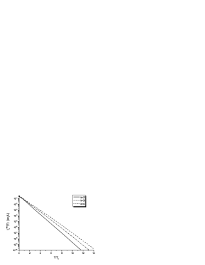
Figure 6: Logarithmic plot of the temperature dependence of the persistent current’s amplitudes in the $k=2,3$ and $4$ parafermion FQH states computed numerically for temperatures in the range $0.03\leq T/T_{0}\leq 14$

Before we derive the high-temperature asymptotics, based on the CFT partition functions for the edge states, let us first announce the result: for $T\gg T_{0}$ the persistent currents amplitudes for the $k=2,3$ and $4$ parafermion FQH states decay exponentially with temperature according to

$$\bar{I}_{k}(T)\ \mathop{\simeq}_{T\gg T_{0}}\ I^{0}_{k}\left(\frac{T}{T_{0}}\right)\exp\left(-\alpha_{k}\frac{T}{T_{0}}\right)$$ (29)

where $I^{0}_{k}$ are constants and the universal exponents $\alpha_{k}$ can be written explicitly in the form

$$\alpha_{k}=\frac{1}{\nu_{H}}+2\Delta^{\mathrm{PF}_{k}}\left(\underline{\Lambda}_{0}+\underline{\Lambda}_{2}\right)=\frac{k+6}{k+2},$$ (30)

where $\nu_{H}$ is the filling factor (1) and $\Delta^{\mathrm{PF}_{k}}\left(\underline{\Lambda}_{0}+\underline{\Lambda}_{2}\right)$ is computed from Eq. (15) for $\sigma=2$.

Remark 3. It is worth-stressing that the universal exponents (30) for the $\mathrm{PF}_{k}$ states are not simply equal to the inverse of the filling factors like it is in the Laughlin states Geller and Loss (1997); Geller et al. (1996, 1997) (see Eq. (2)). There are crucial contributions coming from the neutral sectors which are described here by the ${\mathbb{Z}}_{k}$ parafermion cosets.

Now, let us describe in more detail our analytic computations for the high-temperature regime of the persistent currents in the $\mathrm{PF}_{k}$ states. The high-temperature limit $T\to\infty$ (unlike the low-temperature one) is rather non-trivial since the modular parameter $q=\exp(-2\pi^{2}T_{0}/T)\to 1$ is going outside of the convergence interval for the partition functions and therefore cannot be taken directly. In our case however, one could use the advantage that the complete chiral partition function is constructed as a sum of rational CFT characters, which are covariant under the modular $S$-transformationDi Francesco et al. (1997); Cappelli et al. (2001), i.e.,

$$\chi_{\lambda}(\tau,\zeta)=\sum_{\lambda^{\prime}=1}^{N}S_{\lambda\lambda^{\prime}}\ \chi_{\lambda^{\prime}}(\tau^{\prime},\zeta^{\prime}),$$

where the modular parameters $(\tau,\zeta)$ and $(\tau^{\prime},\zeta^{\prime})$ are related by

$$S:\left|\begin{array}[]{l}\tau=-\frac{1}{\tau^{\prime}}\\ \zeta=-\frac{\zeta^{\prime}}{\tau^{\prime}}\end{array}\right.\quad{\Longleftrightarrow}\quad\left|\begin{array}[]{l}\tau^{\prime}=-\frac{1}{\tau}=i\frac{T}{\pi T_{0}}\\ \zeta^{\prime}=\frac{\zeta}{\tau}=\phi\end{array}\right.$$ (31)

and $S_{\lambda\lambda^{\prime}}$ is called the modular $S$-matrixDi Francesco et al. (1997). In other words, the $S$-transformation could be used to relate the high-temperature and low-temperature limits of the partition function. Note that according to Eq. (31) the usual common phase factor Cappelli and Zemba (1997) in front of the $S$ matrix $S_{\lambda\lambda^{\prime}}$ is trivial since $\exp\left(i\pi\nu_{H}\mathrm{Re}\,({\zeta^{\prime}}^{2}/{\tau^{\prime}})\right)=1$. Now the new modular parameter $q^{\prime}$ vanishes in the high-temperature limit

$$q^{\prime}=\mathrm{e}^{2\pi i\tau^{\prime}}=\exp\left(-\frac{2T}{T_{0}}\right)\to 0\quad\mathrm{when}\quad T\to\infty$$ (32)

so that it would be enough to keep only the leading terms. The partition function (II.1) transforms under the $S$-transformation (31) as follows

$$Z(\tau,\zeta)=\sum_{\lambda=1}^{N}\chi_{\lambda}(\tau^{\prime},\zeta^{\prime})\sum_{\lambda^{\prime}=1}^{N}S_{\lambda\lambda^{\prime}}$$

The quantities $F_{\lambda}=\sum_{\lambda^{\prime}=1}^{N}S_{\lambda\lambda^{\prime}}$ shall play an important role in what follows. Since the complete CFT contains a $u(1)$ factor it turns out that $F_{\lambda}\neq 0$ only if the electric charge of the representation with label $\lambda$ is zero, i.e., $Q_{\mathrm{el}}(\lambda)=0$. In particular, $F_{0}=S_{00}\sum_{i=1}^{N}D_{i}$, where $D_{i}=S_{0i}/S_{00}>0$ are the quantum dimensions Cappelli et al. (2001) of the topological excitations of the FQH fluid.

The explicit form of the modular $S$ matrix for all parafermion FQH states could be obtained Georgiev (2003b) when taking into account the ${\mathbb{Z}}_{k}$ pairing rule and the tensor product structure, Eq. (9), of the parafermion coset CFT. Here we only give the final results that we need for the computation of the persistent currents in the $k=2,3,4$ $\mathrm{PF}_{k}$ states at higher temperatures.

V.1 $k=2$

The $S$-matrix for the $\mathrm{PF}_{2}$ model is labeled by the pairs $(l,\rho)$ where $-1\leq l\leq 2$ and $\rho=0,1$ with the restriction $\rho\geq l-\rho\ \mathrm{mod}\ 2$. Using the explicit form of the $S$ matrix computed according to the general scheme described in Georgiev (2003b) we find that

$$F^{l,\rho}=\sum_{l^{\prime}=-1}^{2}\ \sum_{\rho^{\prime}\geq l^{\prime}-\rho^{\prime}}S^{(l,\rho)}_{(l^{\prime},\rho^{\prime})}=\left\{\begin{array}[]{lcl}\sqrt{2}+1&\mathrm{for}&l=0,\ \rho=0\\ \sqrt{2}-1&\mathrm{for}&l=0,\ \rho=1\\ 0&&\mathrm{otherwise}\end{array}\right.$$

Notice that the $S$-matrix for the $\mathrm{PF}_{2}$ state, which is known as the Pfaffian FQH state, has been explicitly given in a number of papers, see e.g. Ref. Cappelli et al. (1999) and the references therein. Thus, the chiral partition function (11) for $k=2$ after the $S$ transformation (31) can be written as

$$Z_{2}(T,\phi)=(\sqrt{2}+1)\chi_{0,0}(\tau^{\prime},\zeta^{\prime})+(\sqrt{2}-1)\chi_{0,1}(\tau^{\prime},\zeta^{\prime})=$$

$$\simeq\left(\sqrt{2}+1\right)K_{0}(\tau^{\prime},2\zeta^{\prime};8)+\left(\sqrt{2}-1\right)K_{4}(\tau^{\prime},2\zeta^{\prime};8),$$

where we have dropped out a multiplicative $\zeta^{\prime}$-independent term proportional to the central charge, substituted the neutral characters with their leading terms $\mathrm{ch}(\underline{\Lambda}_{0}+\underline{\Lambda}_{0})(\tau^{\prime})\simeq{q^{\prime}}^{0}$, $\mathrm{ch}(\underline{\Lambda}_{1}+\underline{\Lambda}_{1})(\tau^{\prime})\simeq{q^{\prime}}^{1/2}$ and ignored ${q^{\prime}}^{1/2}$ as compared to ${q^{\prime}}^{0}$ since $q^{\prime}\to 0$ when $T\to\infty$. Next, again dropping the $\eta$ function (13) and taking only the leading terms in the $K$ functions, i.e., $n=0$ for $K_{0}(8)$ and $n=0,-1$ for $K_{4}(8)$ one gets

$$Z_{2}(T,\phi)\ \mathop{\simeq}_{T\gg T_{0}}\ \left(\sqrt{2}+1\right)\left(1+2\left(\frac{\sqrt{2}-1}{\sqrt{2}+1}\right)q^{\prime}\cos(2\pi\zeta^{\prime})\right).$$

Substituting $q^{\prime}$ and $\zeta^{\prime}$ with $T$ and $\phi$ according to Eq. (31) and Eq. (32), using the approximation $\ln(1+X)\simeq X$ for $X\ll 1$ and taking the derivative with respect to $\phi$ according to Eq. (17) we get the following high-temperature asymptotic expression for the persistent current ($2\pi^{2}k_{B}T_{0}/\phi_{0}=ev_{F}/L$) in the $\mathrm{PF}_{2}$ state

$$I_{2}(T,\phi)\ \mathop{\simeq}\limits_{T\gg T_{0}}\ -\bar{I}_{2}(T)\sin(2\pi\phi),$$ (33)

$$\bar{I}_{2}(T)=\frac{ev_{F}}{L}\frac{2}{\pi}\left(\frac{\sqrt{2}-1}{\sqrt{2}+1}\right)\frac{T}{T_{0}}\exp\left(-2\frac{T}{T_{0}}\right).$$

Eq. (33) is in agreement with Eqs. (29) and (30) with $\alpha_{2}=2$ being exactly the inverse of the filling factor. This is an accidental exception from the statement in Remark 3 (and in fact the only one in the entire $\mathrm{PF}_{k}$ hierarchy) since for $k=2$ the parafermion CFT dimension $\Delta^{\mathrm{PF}}(\underline{\Lambda}_{0}+\underline{\Lambda}_{2})=0$.

V.2 $k=3$

For this case the sums of the $S$-matrix elements are found to be Cappelli et al. (2001); Georgiev (2003b)

$$F^{l,\rho}=\left\{\begin{array}[]{rcl}\frac{2}{\sqrt{5}}\left(\sin\left(\frac{\pi}{5}\right)+3\sin\left(\frac{2\pi}{5}\right)\right)&\mathrm{for}&l=0,\ \rho=0\\ \frac{2}{\sqrt{5}}\left(3\sin\left(\frac{\pi}{5}\right)-\sin\left(\frac{2\pi}{5}\right)\right)&\mathrm{for}&l=0,\ \rho=2\\ 0&&\mathrm{otherwise}\end{array}\right.$$

(where $-2\leq l^{\prime}\leq 2$, $0\leq\rho^{\prime}\leq 2$ with $\rho^{\prime}\geq l^{\prime}-\rho^{\prime}\ \mathrm{mod}\ 3$) so that the partition function (11) for $k=3$ becomes

$$Z_{3}(T,\phi) = F^{0,0}\chi_{0,0}(\tau^{\prime},\zeta^{\prime})+F^{0,2}\chi_{0,2}(\tau^{\prime},\zeta^{\prime})\simeq$$

$$\simeq K_{0}(\tau^{\prime},3\zeta^{\prime};15)\left(F^{0,0}{q^{\prime}}^{0}+F^{0,2}{q^{\prime}}^{2/5}\right)+$$

$$+ K_{5}(\tau^{\prime},3\zeta^{\prime};15)\left(F^{0,0}{q^{\prime}}^{2/3}+F^{0,2}{q^{\prime}}^{1/15}\right)+$$

$$+ K_{-5}(\tau^{\prime},3\zeta^{\prime};15)\left(F^{0,0}{q^{\prime}}^{2/3}+F^{0,2}{q^{\prime}}^{1/15}\right),$$

where we have used (skipping the central charge term in the characters (14) like in the previous subsection) that $\mathrm{ch}(\underline{\Lambda}_{0}+\underline{\Lambda}_{0})(\tau^{\prime})\simeq{q^{\prime}}^{0}$, $\mathrm{ch}(\underline{\Lambda}_{0}+\underline{\Lambda}_{1})(\tau^{\prime})=\mathrm{ch}(\underline{\Lambda}_{0}+\underline{\Lambda}_{2})(\tau^{\prime})\simeq{q^{\prime}}^{1/15}$, $\mathrm{ch}(\underline{\Lambda}_{1}+\underline{\Lambda}_{1})(\tau^{\prime})=\mathrm{ch}(\underline{\Lambda}_{2}+\underline{\Lambda}_{2})(\tau^{\prime})\simeq{q^{\prime}}^{2/3}$ and $\mathrm{ch}(\underline{\Lambda}_{1}+\underline{\Lambda}_{2})(\tau^{\prime})\simeq{q^{\prime}}^{2/5}$. Keeping only the lowest powers in $q^{\prime}\to 0$, ignoring the Dedekind function (13) and taking only $n=0$ in the $K$ functions we get

$$Z_{3}(T,\phi)\ \mathop{\simeq}_{T\gg T_{0}}\ F^{0,0}\left(1+2\frac{F^{0,2}}{F^{0,0}}\,{q^{\prime}}^{\frac{1}{2}\left[5/3+2/15\right]}\cos(2\pi\zeta^{\prime})\right)$$

To get the persistent current in the high-temperature limit we apply the same scheme as for $k=2$ in Sect. V.1 which yields

$$I_{3}(T,\phi)\mathop{\simeq}\limits_{T\gg T_{0}}-\bar{I}_{3}(T)\sin(2\pi\phi),$$ (34)

$$\bar{I}_{3}(T)=\frac{ev_{F}}{L}\frac{2}{\pi}\left(\frac{D-1}{D+1}\right)\frac{T}{T_{0}}\exp\left(-\frac{T}{T_{0}}\left[\frac{5}{3}+\frac{2}{15}\right]\right),$$

where we have transformed the ratio $F^{0,2}/F^{0,0}$ in the form

$$\frac{F^{0,2}}{F^{0,0}}=\frac{D-1}{D+1},\quad\mathrm{with}\quad D=2\cos\left(\frac{\pi}{5}\right)$$

being the quantum dimension Cappelli et al. (2001) of the elementary quasihole in the $\mathrm{PF}_{3}$ FQH state.

V.3 $k=4$

The $S$-matrix elements for the $\mathrm{PF}_{4}$ FQH state have been computed in Ref. Georgiev (2003b). The quantities $F^{l,\rho}$ can be written as follows

$$F^{l,\rho}=\sum_{l^{\prime}=-2}^{3}\ \sum_{\rho^{\prime}\geq l^{\prime}-\rho^{\prime}}S^{(l,\rho)}_{(l^{\prime},\rho^{\prime})}=\left\{\begin{array}[]{rcl}2+\sqrt{3}&\ \mathrm{for}&l=0,\ \rho=0\\ 2-\sqrt{3}&\ \mathrm{for}&l=0,\ \rho=2\\ 1&\ \mathrm{for}&l=0,\ \rho=3\\ 0&&\ \mathrm{otherwise}\end{array}\right.$$

so that the partition function (11) for $k=4$ becomes

$$Z_{4}(T,\phi)=$$

$$=F^{0,0}\chi_{0,0}(\tau^{\prime},\zeta^{\prime})+F^{0,2}\chi_{0,2}(\tau^{\prime},\zeta^{\prime})+F^{0,3}\chi_{0,3}(\tau^{\prime},\zeta^{\prime})$$

$$\simeq K_{0}(24)\left(F^{0,0}{q^{\prime}}^{\Delta^{\mathrm{PF}}(0,0)}+F^{0,2}{q^{\prime}}^{\Delta^{\mathrm{PF}}(2,2)}+F^{0,3}{q^{\prime}}^{\Delta^{\mathrm{PF}}(1,3)}\right)+$$

$$+K_{6}(24)\left(F^{0,0}{q^{\prime}}^{\Delta^{\mathrm{PF}}(1,1)}+F^{0,2}{q^{\prime}}^{\Delta^{\mathrm{PF}}(3,3)}+F^{0,3}{q^{\prime}}^{\Delta^{\mathrm{PF}}(0,2)}\right)+$$

$$+K_{-6}(24)\left(F^{0,0}{q^{\prime}}^{\Delta^{\mathrm{PF}}(3,3)}+F^{0,2}{q^{\prime}}^{\Delta^{\mathrm{PF}}(1,1)}+F^{0,3}{q^{\prime}}^{\Delta^{\mathrm{PF}}(0,2)}\right),$$

where $K_{l}(24)=:K_{l}(\tau^{\prime},4\zeta^{\prime};24)$ and we have used $\mathrm{ch}(\underline{\Lambda}_{\mu}+\underline{\Lambda}_{\rho})(\tau^{\prime})\simeq{q^{\prime}}^{\Delta^{\mathrm{PF}}(\mu,\rho)}$, with $\Delta^{\mathrm{PF}}(0,0)=0$, $\Delta^{\mathrm{PF}}(0,2)=1/12$, $\Delta^{\mathrm{PF}}(1,1)=\Delta^{\mathrm{PF}}(3,3)=3/4$, $\Delta^{\mathrm{PF}}(1,3)=1/3$, $\Delta^{\mathrm{PF}}(2,2)=1$, again skipping the central charge term in the characters (14). The explicit form of the CFT dimensions $\Delta^{\mathrm{PF}}(\mu,\rho)$ for the parafermion coset $\mathrm{PF}_{k}$, defined in Eq. (9), can be found in Ref. Cappelli et al. (2001).

Keeping only the lowest powers in $q^{\prime}\to 0$, ignoring the Dedekind function (13) and taking only $n=0$ in the $K$ functions we get

$$Z_{4}(T,\phi)\ \mathop{\simeq}_{T\gg T_{0}}\ F^{0,0}+2F^{0,3}{q^{\prime}}^{\frac{3}{4}+\Delta^{\mathrm{PF}}(0,2)}\cos(2\pi\zeta^{\prime})$$

To get the persistent current in the high-temperature limit we apply the same scheme as in Sect. V.1 obtaining

$$I_{4}(T,\phi)\ \mathop{\simeq}\limits_{T\gg T_{0}}\ -\bar{I}_{4}(T)\sin(2\pi\phi),$$

$$\bar{I}_{4}(T)=\frac{ev_{F}}{L}\frac{2}{\pi}\left(\frac{1}{2+\sqrt{3}}\right)\frac{T}{T_{0}}\ \exp\left(-\frac{T}{T_{0}}\left[\frac{3}{2}+\frac{2}{12}\right]\right).$$ (35)

Finally, we can extrapolate the high-temperature results Eqs. (33), (34) and (V.3) for the $k=2$, $3$ and $4$ $\mathrm{PF}_{k}$ states to the entire parafermion hierarchy. The universal exponent (30) for any FQH state can be extracted from the CFT operator content and the modular $S$-matrix. In our case, the analysis in Sects. V.1, V.2 and V.3 implies that the neutral contribution to the exponent is exactly equal to twice the minimal CFT dimension of the neutral field, that we shall label by $\underline{\Lambda}_{*}$, whose character is coupled to $K_{\pm k+2}(\tau^{\prime},\kappa\zeta^{\prime};k(k+2))$, i.e., $\alpha=1/\nu_{H}+2\Delta^{\mathrm{PF}}(\underline{\Lambda}_{*})$, where $\underline{\Lambda}_{*}$ is determined Georgiev (2003b) from the pairing rule condition

$$P[\underline{\Lambda}_{*}]\equiv k+2\ \mathrm{mod}\ k\quad\mathrm{with}\quad\Delta^{\mathrm{PF}}(\underline{\Lambda}_{*})=\min.$$

For the $\mathrm{PF}_{k}$ states $P$ is the ${\mathbb{Z}}_{k}$ charge and it is easy to see that $\underline{\Lambda}_{*}=\underline{\Lambda}_{0}+\underline{\Lambda}_{2}$ for all $k$ in the above equation and that the formula (30) for $\alpha_{k}$ is valid for all parafermion FQH states.

Instead of plotting together for comparison the analytic high-temperature asymptotic curves and the exact numerical ones (the latter being shown on Fig. 6), we have computed numerically the values of $\alpha_{k}$ and $I^{0}_{k}$ for the $k=2,3,4$ PF states by Least-Squares Linear Regression of the logarithmic amplitude $\ln\left(\bar{I}_{k}(T)\right)-\ln(T/T_{0})$ over 80 points in the interval $6\leq T/T_{0}\leq 14$. It is worth-noting that after subtracting the $\ln(T/T_{0})$ contribution from the (numerical) logarithmic amplitude the latter becomes an almost perfect straight line as a function of $T$. The exact and numerical values of the exponents $\alpha_{k}$ (the slopes in the logarithmic plots) and the asymptotic amplitudes $I^{0}_{k}$ (the extrapolated $y$-intercepts) for the first several $\mathrm{PF}_{k}$ states are summarized in Table 1.

Table 1: The slopes $\alpha_{k}$ and the $y$-intercepts $I^{0}_{k}$ (in units $ev_{F}/L$) of the logarithmic plots in the high-temperature region for the $k=2,3,4$ PF states. The numerical values have been extracted from the numerical data for $6\leq T/T_{0}\leq 14$ using the Least-Square linear regression while the corresponding exact quantities have been taken from Eqs. (33), (34) and (V.3).

$k$	$\alpha_{k}$		$I^{0}_{k}$ $\ [ev_{F}/L]$
	numeric	exact	numeric	exact
$2$	$2.00071$	$2$	$0.11025$	$(2/\pi)(\sqrt{2}-1)/(\sqrt{2}+1)$
$3$	$1.80001$	$9/5$	$0.15031$	$(2/\pi)(2\cos(\pi/5)-1)/(2\cos(\pi/5)+1)$
$4$	$1.66631$	$5/3$	$0.16983$	$(2/\pi)/(2+\sqrt{3})$

The amazing overlap between the exact and numerical values of $\alpha_{k}$ and $I^{0}_{k}$ shown in Table 1 gives us the conviction that the leading order approximations made in Sects. V.1, V.2 and V.3 are fairly reasonable and the belief that the modular $S$-matrix could play an important role in the computation of certain thermodynamic quantities.

Eq. (29) suggests the existence of another mechanism which reduces the persistent currents amplitudes at high temperature, as already mentioned at the end of Sect. III. The point is that the finite temperature introduces a length scaleGeller and Loss (1997), the thermal length $L_{T}=\hbar v_{F}/k_{B}T$ and when, for higher temperatures this length becomes smaller than the circumference $L$ of the ring the persistent currents vanish exponentially with $L/L_{T}$ due to decoherence effects. Following the convention of Ref. Geller and Loss (1997) we take as a characteristic temperature $T_{0}$ according to Eq. (7) so that

$$\frac{T}{T_{0}}=\pi\frac{L}{L_{T}}$$

and the relation with the coherence length $L_{\varphi}$ can be estimated as $L_{T}\simeq 2\pi L_{\varphi}$ for the experimental setup of Ref. Mailly et al. (1993) at $T=15$ mK.

VI The periods of the persistent currents for the PF states

The low- and high- temperature asymptotics of the persistent currents investigated in Sect. IV and Sect. V as well as the numerical calculations performed for temperatures in the range $0.03\leq T/T_{0}\leq 14$ unambiguously show that these currents are periodic functions of the AB flux with period exactly one flux quantum. This is in agreement with the Bloch–Byers–Yang theorem discussed in the Introduction. On the other hand, our result is at variance with recent theoretical proposals Ino (2003); Kiryu (2002) that the currents have fractional period $1/k$ for the $\mathrm{PF}_{k}$ states (without contradicting the Bloch theorem). Note that a fractional periodicity, such as $1/2$, $1/3$ etc., of the persistent currents would be a signal for some broken continuous symmetry Deo et al. (2001). However, in incompressible (i.e., effectively $1+1$ dimensional) electron systems, described by unitary effective field theories in $1+1$ dimensions, a spontaneous breaking of rotational symmetry can occur only at zero temperature Mermin and Wagner (1966); Coleman (1973); Geller (2001). One important consequence of our main result confirming that the period of the persistent currents in the $\mathrm{PF}_{k}$ states is exactly $1$ is that it rules out any possibility for a spontaneous breaking of continuous symmetries at finite temperature. Nevertheless, it may be possible that the FQH systems undergo phase transitionsGeller (2001) at $T=0$ to some BCS-like phases where the periods could be less than $1$.

For the analysis of the periods of the persistent currents we have extracted from the numerical data and plotted on Fig. 7 the position of the unique maximum $\phi_{\max}$ for $-1/2\leq\phi\leq 1/2$ of the persistent currents for the $k=2$, $3$ and $4$ $\mathrm{PF}_{k}$ states as functions of $T$ in the region $0.03\leq T/T_{0}\leq 3$. Obviously, the position of the maximum tends to $-1/2$ for $T\to 0$, in perfect agreement with Eq. (26) (we skipped the low-temperature asymptotic curves for $k=2,3,4$ that could be plotted from this equation because they become indistinguishable from the numerical ones for $T/T_{0}<0.5$).

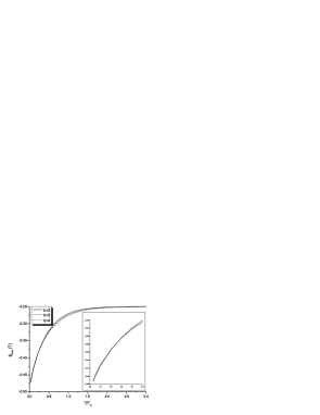
Figure 7: The position of the maximum of the persistent currents in the $k=2,3$ and $4$ parafermion FQH states computed numerically  for temperatures $0.03\leq T/T_{0}\leq 3$. The inset shows a more detailed plot for lower temperatures.

For temperatures $T\gg T_{0}$ the position $\phi_{\max}$ tends quickly to $-1/4$, this time in good agreement with Eqs. (33), (34) and (V.3).

Should the period of the currents be smaller than $1$, e.g., $1/k$ for the $\mathrm{PF}_{k}$ states, the low-temperature position of the maximum must be

$$\left|\phi_{\max}(T)\right|<\frac{1}{2k},\quad\mathrm{for}\quad T\ll T_{0}.$$

because the persistent currents become for $T\to 0$ odd linear functions of the flux $\phi$. In order to have period $1/k$ for the $\mathrm{PF}_{k}$, with $k=2,3,4,\ldots$, it is necessary that $|\lim_{T\to 0}\phi_{\max}(T)|\leq 1/2k$. This would obviously be in contradiction with the numerical results that we have presented here showing that

$$\left|\lim_{T\to 0}\phi_{\max}(T)\right|=\frac{1}{2}.$$

Therefore, we conclude that our numerical data suggests that the periods of the persistent currents for the $\mathrm{PF}_{k}$ states cannot be fractional.

Another point we want to stress is that according to Eq. (26) the position of the maximum is independent of the filling factor for $T\ll T_{0}$ and depends only on the ratio between the quasihole’s CFT dimension and its electric charge.

VII Conclusion

We have proposed a general scheme for the incorporation of the Aharonov–Bohm flux in the effective conformal field theory for the edge states of a mesoscopic disk or annulus FQH sample, which opens the possibility to study the mesoscopic effects from the CFT point of view. This approach is based on a special invariance condition (5) representing the Laughlin spectral flow and its generalization (6) in the CFT framework.

The persistent currents and magnetic susceptibilities can be computed explicitly using the extended $V$ transformation (6) and the Cappelli–Zemba factors (8). We have calculated numerically the persistent currents and magnetic susceptibilities for the parafermion FQH states in the second Landau level and have analyzed their flux periodicities and temperature behavior. The numerical results have been presented in several figures. One of our most important observation is that the periods of the persistent currents and magnetic susceptibilities are exactly one flux quantum for all numerically accessible temperatures $0.03\leq T/T_{0}\leq 14$, which leaves no room for a spontaneous breaking of continuous symmetries.

On the other hand, we have obtained analytic asymptotic expressions, Eqs. (27), (28) and (29), for the low- and high-temperature limits of the partition functions, persistent currents amplitudes and zero-field magnetic susceptibilities in the parafermion FQH states, which are in excellent agreement with our numerical data in the corresponding regimes. These expressions carry important information about the neutral properties of the FQH fluid and reveal two different mechanisms reducing the persistent currents at low- and high- temperatures respectively, which are in agreement with the phenomenological expectations Mailly et al. (1993). Our conclusion is that the asymptotic behavior of the persistent currents in both regimes in mesoscopic FQH states can be used to distinguish between different CFTs for the same filling factor. In particular, the universal exponent (30) and the proper quasihole energy (21) completely characterize the neutral properties of the FQH system and together with the filling factor and the minimal quasiparticle electric charge unambiguously determine the FQH universality class. Surprisingly the universal exponent (30) for the high-temperature decay of the persistent currents amplitudes for the PF states turned out to be determined not simply by the filling factor, like in the Laughlin states, but having also a crucial contribution from the neutral sector.

A similar analysis could be performed e.g. for the (principle) Jain series of filling factors where several different CFT have been proposed to describe the same electric properties while differing significantly in the neutral sectors.