Charge-density-wave instabilities driven by multiple umklapp scattering

Abstract

We show that the concept of umklapp-scattering driven instabilities in one-dimensional systems can be generalized to arbitrary multiple umklapp-scattering processes at commensurate fillings given that the system has sufficiently longer range interactions. To this end we study the fundamental model system, namely interacting spinless fermions on a one-dimensional lattice, via a density matrix renormalization group approach. The instabilities are investigated via a new method allowing to calculate the ground-state charge stiffness numerically exactly. The method can be used to determine other ground state susceptibilities in general.

I Introduction

The relevance of umklapp-scattering terms in one-dimensional systems with commensurate filling has long been established.Soly79 Besides the general theoretical interest in one-dimensional systems because of the existing exact solutions to some of them KM97 and the field-theoretical description of the low energy physics,GNT98 the application of one-dimensional models to the rich phase diagrams of quasi one-dimensional systems such as the Bechgaard and Fabre salts Bour00 has a long standing history. The degeneracy of the ground state leads to the presence of solitonic excitations in the one-dimensional systems and recent studies focus on the question to what extent these collective modes are observable ET02 in the systems under investigation.

Here we focus on the generic instabilities of systems of fermions without the internal magnetic degree of freedom. The Hamiltonian under consideration is

$$H=-t\sum_{l=1}^{M}\left(c^{\dagger}_{l+1}c^{\phantom{\dagger}}_{l}+{\rm h.c.}\right)+\sum_{s=1}^{s_{\rm max}}V_{s}\sum_{l}n_{l}n_{l+s}\,,$$ (1)

with fermionic creation ($c^{\dagger}_{l}$) and annihilation ($c^{\phantom{\dagger}}_{l}$) operators at site $l$, nearest-neighbor hopping amplitude $t$, density-density interaction amplitude $V_{s}$ between fermions on sites of separation $s$ and density operators $n_{l}=c^{\dagger}_{l}c^{\phantom{\dagger}}_{l}$. Energies are given in units of $t$. The decay of the interaction with distance requires in general $V_{s+1}<V_{s}$, with the exception of zig-zag chains and some spin systems where the nearest-neighbor interaction is suppressed by the lattice geometry. We apply periodic boundary conditions, i.e., $c_{M+1}\equiv c_{1}$.Antiquote The model in Eq. (1) is directly applicable to spin 1/2 chains that can be mapped onto chains of spinless fermions.ETD97 Furthermore, its widely studied continuum representation Hald82b is similar to the charge sector of the bosonized Hubbard model.ET02 ; YTS01 Finally, Eq. (1) allows to study the interplay of ordered phases with different modulation wave vectors, which proves useful for the understanding of materials that exhibit multiple phase transitions.RP99

The purpose of this paper is threefold. (i) We present a novel method to determine the ground-state curvature or, equivalently, the ground-state charge stiffness. (ii) The approach allows for an accurate identification of charge-density-wave (CDW) instabilities at commensurate fillings. The phase diagrams for various relevant sets of parameters are shown. (iii) We discuss the physical insight that can be gained from the continuum representation of Eq. (1) and by comparison with the numerical results show the importance of lattice effects.

To this end we present a detailed density matrix renormalization group (DMRG) study DMRG of the lattice model Eq. (1). Sufficiently large system sizes are accessible to model the thermodynamic limit without the shortfall of neglecting possible lattice effects.

II Numerical approach

The ground state curvature $C$ is defined as

$$C=M\left.\frac{\partial^{2}E_{0}(\phi)}{\partial\phi^{2}}\right|_{\phi=0},$$ (2)

where $\phi$ is a magnetic flux that penetrates our system which is closed to a ring. The magnetic flux inside the ring can be gauged into a single bond leading to twisted boundary conditions $c_{1}={\rm e}^{\imath\phi}c_{M+1}$. According to Kohn Kohn64 $C$ is equivalent to the Drude weight of the $T=0$ dc conductivity. The curvature in Eq. (2) is the second order coefficient of the Taylor series of $E_{0}(\phi)$, i.e., $E_{0}(\phi)=E_{0}(0)+E^{(1)}\phi+\frac{C}{2M}\phi^{2}+O(\phi^{3})$. In order to compute the coefficient exactly we expand $H(\phi)$ and the ground-state wave function $|{\Psi_{0}(\phi)}\rangle$ at $\phi=0$ in second order. $H$ is given via

$$H(\phi)=H^{(0)}+\imath\phi J-\frac{\phi^{2}}{2}T+{\rm O}(\phi^{3})\,,\\$$ (3)

where $H^{(1)}=\imath J$ is the current operator with

$$J=c^{\dagger}_{M}c^{\phantom{\dagger}}_{1}-c^{\dagger}_{1}c^{\phantom{\dagger}}_{M}$$ (4)

and

$$T=H^{(2)}=-(c^{\dagger}_{M}c^{\phantom{\dagger}}_{1}+c^{\dagger}_{1}c^{\phantom{\dagger}}_{M})$$ (5)

is the kinetic energy on the bond between the $M$th and first site. Due to the normalization of the wave function $\langle{\Psi(\phi)}\mid{\Psi(\phi)}\rangle=1=\langle{\Psi^{(i)}}\mid{\Psi^{(i)}}\rangle$ the first order correction $|{\Psi^{(1)}}\rangle$ in the expansion $|{\Psi(\phi)}\rangle=|{\Psi^{(0)}}\rangle+\phi|{\Psi^{(1)}}\rangle+{\rm O}(\phi^{2})$ is orthogonal to the ground state $|{\Psi^{(0)}}\rangle$ at zero flux and is obtained by solving the set of linear equations

$$\left(H^{(0)}-E^{(0)}_{0}\right)|{\Psi^{(1)}}\rangle=\left(E^{(1)}-\imath J\right)|{\Psi^{(0)}}\rangle\,.$$ (6)

on the subspace that is orthogonal to the ground state. The resulting curvature is given by

$$C=M\langle{\Psi^{(0)}}|T|{\Psi^{(0)}}\rangle+2M\langle{\Psi^{(0)}}|\imath J-E^{(1)}|{\Psi^{(1)}}\rangle$$ (7)

with $E^{(1)}=\langle{\Psi^{(0)}}|H^{(1)}|{\Psi^{(0)}}\rangle$.

It must be stressed that this approach is exact. Therefore the accuracy of our numerical results is only limited by the truncation error of the DMRG. Consequently any ambiguity in the determination of $C$ incurred through a numerical finite difference approximation of the derivative of $E_{0}(\phi)$ is avoided. Moreover, our procedure allows to calculate $C$ without referring to a system with a finite flux that could destroy the commensurability effects we want to measure.

For systems with time-reversal symmetry and a nondegenerate ground state one finds $E^{(1)}=0$ and from Eq. (6) follows that $|{\Psi^{(1)}}\rangle$ is purely imaginary. In turn it follows that $C$ can be calculated by using real numbers only. Therefore solving the linear set of equations (6) and storing the additional target vectors ${\rm Im\,}|{\Psi^{(1)})}\rangle$ and $J|{\Psi^{(1)})}\rangle$ are outweighed by the fact that we can restrict ourselves to real numbers. Since $\langle{\Psi^{(1)}}\mid{\Psi^{(0)}}\rangle=0$, solving Eq. (6) is stable and can be performed by a mixture of standard preconditioned minimal residue and conjugate gradient methods which we extended by a projection on the space orthogonal to the subspace of the ground state(s). The extension to degenerate ground states is straightforward and can be performed similar to Brillouin-Wigner perturbation theory.Zima69 For the small systems ($M<30$) we keep 300 to 400 states per block $A$ and $B$, while we keep up to 1000 states per block for the larger systems. In addition to the ground state $|{\Psi^{(0)}}\rangle$ and the auxiliary states $J|{\Psi^{(0)}}\rangle$ and $|{\Psi^{(1)}}\rangle$ we target at least for the first four excited eigenstates to treat degeneracies properly.

III Phase diagrams

In order to investigate the general features the model in Eq. (1) we study its phase diagram as a function of the nearest- ($V_{1}$) and next-nearest-neighbor ($V_{2}$) interaction. The result is presented in Fig. 1, where the curvature is plotted versus $V_{1}$ and $V_{2}$. Charge order implies $C(V_{1},V_{2})=0$. In Fig. 1(a) the system is shown at half filling for a chain of length 32. In CDW phase I the ground state is twofold degenerate Finitequote with ordering pattern ($\bullet$$\circ$$\bullet$$\circ$) and ($\circ$$\bullet$$\circ$$\bullet$). Here $\circ$ denotes a vacant and $\bullet$ denotes an occupied site. In phase II the ground state is fourfold degenerate with ordering pattern ($\bullet$$\bullet$$\circ$$\circ$), ($\circ$$\bullet$$\bullet$$\circ$), ($\circ$$\circ$$\bullet$$\bullet$), and ($\bullet$$\circ$$\circ$$\bullet$). The transition between phases I and II along the line $V_{1}=2V_{2}$ is expected from simple potential energy arguments for the corresponding real-space ground-state configurations. The finite width of the uniform region is due to a gain in kinetic energy near the line $V_{1}=2V_{2}$, where the charge ordering effects are reduced by the competition of the two potential energies. Figure 1(b) shows the curvature of a chain of length 24 at $1/3$ filling. The ordered phase is observed for sufficiently large values of $V_{1},V_{2}\ \raisebox{-3.01385pt}{$\stackrel{{\scriptstyle\mbox{$>$}}}{{\sim}}$}\ 4$ and has a triply degenerate ground state with ordering pattern ($\bullet$$\circ$$\circ$$\bullet$$\circ$$\circ$), ($\circ$$\bullet$$\circ$$\circ$$\bullet$$\circ$), and ($\circ$$\circ$$\bullet$$\circ$$\circ$$\bullet$).

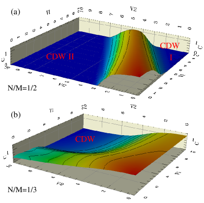
Figure 1: Curvature of the (a) half and (b) one-third-filled chain with (a) $M=32$ and (b) $M=24$ sites as a function of the nearest- ($V_{1}$) and next-neares-neighbor ($V_{2}$) interaction strength. Charge order implies $C=0$. The ordering pattern are discussed in the text. In (a) the CDW phase I doubles the unit cell, phase II quadruples the unit cell and the ground states are twofold and fourfold degenerate, respectively. In (b) the ordered phase triples the unit cell with triply degenerate ground state.

Figure 2 shows the finite size effects of the curvature at half filling via cuts through Fig. 1(a) for various system sizes. Figure 2(a) shows $C(V_{1},0)$, panel (b) $C(0,V_{2})$, and panel (c) $C(V_{1},10-2V_{1})$. For $V_{2}=0$ and $M\to\infty$ it is known from Bethe anstatz calculationsdCG66 that in the ordered phase for $V_{1}>V_{1,\rm c}=2$ an excitation gap opens exponentiallyYY66c as $\sim\exp\left(-\pi^{2}/\sqrt{8(V_{1}-V_{1,\rm c})}\right)$. As a result the convergence of the curvature to the thermodynamic limit in CDW I near the transition point is very slow [Fig. 2(a) and Ref. LCS01, ]. In contrast we find a gap in CDW II obeying the power law $\Delta_{\rm II}\big{|}_{V_{1}=0}\sim(V_{2}-V_{2,\rm c})^{3/4}$ as shown in the inset of Fig. 2(c). The reason for the different behavior lies in the bond-ordered phase (BO) equivalent to that found in frustrated Heisenberg chains,SA01 which we find strong evidence for between the Luttinger liquid (LL) and CDW II phases, see Fig. 2(d).

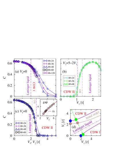
Figure 2: Curvature at half filling as a function of the interaction parameters for different system sizes along cuts through Fig. 1(a). Panel (a) $V_{2}=0$. Panel (b) $V_{2}=5-2V_{1}$. Panel (c) $V_{1}=0$, the inset shows that the gap in CDW II opens as $\Delta_{\rm II}\sim(V_{2}-V_{2,\rm c})^{3/4}$. Panel (d) shows a sketch of the resulting phase diagram. The dashed line indicates the direction of the cut shown in panel (b), the dash-dotted lines shows $2V_{2}=V_{1}$. Dots mark the transition points determined herein.

The numerical determination of the critical values of the interaction is difficult because of the smallness of the gap near the transitions. It turns out though that the finite size effects of $M(E_{1}-E_{0})$ change sign at the phase transition between the LL and the ordered BO and CDW I phases, i.e., $\lim_{M\to\infty}\partial M(E_{1}-E_{0})/(\partial M)|_{V_{1}=V_{1,c}}=0$. On the other hand, in the CDW II phase systems with sizes $M{\rm mod}4=0$ have much smaller finite size effects than for $M{\rm mod}4=2$ while in the BO phase both are equivalent. Moreover, the systems exhibit well defined level crossings between the bond ordered and the CDW phases.SA01 The effects are illustrated in Fig. 3 for $M=24$ (diamonds), $M=36$ (crosses), and $M=48$ (triangles) for a cut along the line $V_{2}=5-2V_{1}$ for the four lowest excited states. Lines are guides to the eye. Note that for the actual parameter determination systems of sizes up to 60 sites where studied near the phase transitions.

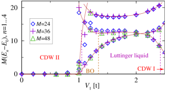
Figure 3: Level crossings at the phase boundaries between the BO and CDW II phase and changes of sign of the finite size effects of $M(E_{1}-E_{0})$ at the boundaries of the LL phase along the line $V_{2}=5-2V_{1}$. System sizes are $M=24$ (diamonds), $M=36$ (crosses) and $M=48$ (triangles). Lines are guides to the eye.

Combining different approaches we estimate for $V_{1}=0$ a value of $V_{2,\rm c}=2.66\pm 0.1$ while along the line $V_{2}=5-2V_{1}$ the critical points into the CDW phases are $(V_{1,\rm c},V_{2,\rm c})\in\{(1.05\pm 0.05,2.9\pm 0.1);(2.4\pm 0.05,0.2\pm 0.1)\}$. The transitions from the LL to the BO phase occur at $(V_{1,\rm b},V_{2,\rm b})=(0,2.15\pm 0.1)$ and $(1.35\pm 0.05,2.3\pm 0.1)$. The resulting phase diagram is sketched schematically in Fig. 2(d). Thick dots are transition values determined numerically within this work. The numerical analysis for large values of $V^{*}=20,50,100$ with $V_{2}=V^{*}-2V_{1}$ suggests that for $V^{*}\gg t$ the uniform region (BO and LL phases) between CDW I and CDW II extends along the line $V_{1}=2V_{2}$ with a width of $\sim\sqrt{5}\,t$.3phasesquote At sufficiently high interaction strength the LL phase disappears. The triple point between the BO, LL, and CDW I phase can be estimated to be near $(V_{1,\rm t},V_{2,\rm t})\approx(8.2,3.6)$, see also Sec. V.

IV Commensurability effects

Any deviation from commensurate filling in one-dimensional systems leads to the presence of solitonic excitations even at zero temperature which disorder the system due to the degeneracy of the ground state.ET02 Our approach allows to demonstrate the sensitivity of our one-dimensional model system to the commensurability of the filling very nicely as is shown in Fig. 4. The diamonds show the curvature for different fillings at different system sizes $18\leq M\leq 60$ for $V_{1}=10$ and $V_{2}=3$, i.e., the system is charge ordered both for fillings of $1/2$ and $1/3$ as can be seen from Figs. 1(a) and 1(b). Since the values of interaction are such that the system at $N/M=1/3$ is close to the transition to the non-ordered phase the convergence is slow at that point. The squares show the curvature for $V_{1}=10$ and $V_{2}=5$, where no charge ordering is observed at half filling due to the competition between $V_{1}$ and $V_{2}$. Note that the results are symmetric about $N/M=1/2$ because of particle-hole symmetry.

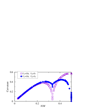
Figure 4: Curvature as a function of filling for different numbers of fermions $2\leq N\leq M/2$ at system sizes $18\leq M\leq 60$. Diamonds: $V_{1}=10$ and $V_{2}=3$ with charge order at $N/M=1/2$ and $N/M=1/3$. Squares: $V_{1}=10$ and $V_{2}=5$ with charge order only at $N/M=1/3$ (c.f. Fig. 1).

The results for $V_{1},V_{2}\neq 0$ discussed in detail above can readily be generalized to systems with longer range interaction. For example, for $V_{1},V_{2},V_{3}\neq 0$ and sufficiently large $V_{3}$ we find a phase with ordering pattern ($\bullet$$\circ$$\circ$$\circ$) and four-fold-degenerate ground state at quarter filling. Since a detailed discussion would be a simple extension of the case studied above it is omitted here. The crucial result that follows from the generalization is that for all systems under investigation ($s_{\rm max}=1,2,3,4,5$) an instability at commensurate filling $N/M$ is only observed for sufficiently long-ranged interaction, i.e., $V_{s}\neq 0\ \forall\ s\leq s_{\rm max}$ with $s_{\rm max}=M/N-1$. The case of $s_{\rm max}=5$ is illustrated in Fig. 5 for $V_{1}=120$, $V_{2}=60$, $V_{3}=30$, $V_{4}=15$, and $V_{5}=6$ and exhibits charge density instabilities only for $N/M\geq 1/6$. Note that for sufficiently strong interaction there are also second-harmonic anomalies such as the one at $N/M=2/5$ in Fig. 5.

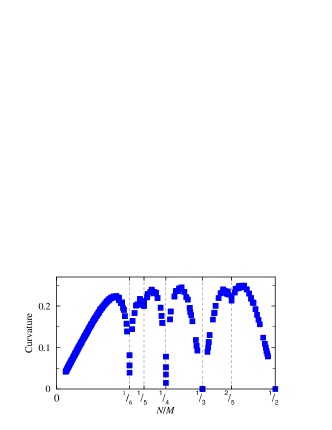
Figure 5: Curvature for $s_{\rm max}=5$ as a function of filling for different numbers of fermions $2\leq N\leq M/2$ at system sizes $20\leq M\leq 48$ with $V_{1}=120$, $V_{2}=60$, $V_{3}=30$, $V_{4}=15$, and $V_{5}=6$ with charge order instabilities at $N/M=1/6$, $N/M=1/5$, $N/M=1/4$, $N/M=1/3$, and $N/M=1/2$. Note that for the strong interactions under investigation there is also a second-harmonic anomaly at $N/M=2/5$. The result supports the notion that instabilities occur only at fillings with $N/M\geq 1/(s_{\rm max}+1)$.

The notion of instabilities only for sufficiently long ranged interaction is quite intuitive when considering the system under investigation in real space, because the system cannot order when the mean distance between particles is larger than the interaction range.

V Continuum representation

The low energy properties of the Hamiltonian Eq. (1) can be approximated by its field-theoretical equivalent obtained by the standard Abelian bosonization technique.GNT98 ; Hald82b The kinetic and forward-scattering parts lead to the free Hamiltonian

$${\cal H}_{0}=\frac{v}{16\pi}\int_{-\infty}^{\infty}dx\left(K\ \Pi^{2}+\frac{1}{K}\left(\partial_{x}\,\phi\right)^{2}\right)$$ (8)

with excitation velocity $v$, Luttinger liquid parameter $K$, Bose fields $\phi(x)$, and their conjugate momenta $\Pi(x)$. The continuum coordinate is $x=\lim_{a\to 0}la$ with the lattice constant $a$ and $M\to\infty$. The umklapp-scattering part is

$${\cal H}_{\rm u}=\lim_{a\to 0}\sum_{s}\frac{V_{s}}{2(\pi a)^{2}}\int_{-\infty}^{\infty}dx\cos\left[\sqrt{2}\phi-(4k_{\rm F}-G)x\right]$$ (9)

with Fermi wave vector $k_{\rm F}=\pi\rho/a$ where $\rho=N/M\leq 1$ is the number of fermions per site. $G$ is a reciprocal lattice vector. For sufficiently small $K<1/2$ and if $4k_{\rm F}=2\pi/a$, Eq. (9) yields a relevant contribution to the total Hamiltonian ${\cal H}={\cal H}_{0}+{\cal H}_{\rm u}$ which then represents a sine-Gordon model.YTS01 Indeed, using the finite-size scaling of the ground-state energy per site in the LL phase KBI93 ; SA01 $\frac{E_{0}(M)}{M}=e(\infty)-\frac{\pi}{6M^{2}}v$, where $v$ is the velocity of the elementary excitations, and the relation $C=\frac{v}{\pi}K$ we find $K>1/2$ in the LL phase, $K\approx 1/2$ at the LL-phase boundary, and $K<1/2$ elsewhere within the numerical precision of the methodSA01 of about $\pm 5$%. The latter can be estimated at $V_{1}=2$ and $V_{2}=0$. This is illustrated in Fig. 6 for cuts along $V_{2}=5-2V_{1}$ (circles), $V_{2}=10-2V_{1}$ (triangles), and $V_{2}=20-2V_{1}$ (diamonds) and confirms the applicability of Eqs. (8) and (9) for $\rho=1/2$.

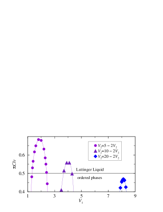
Figure 6: Numerical estimate $\pi C/v$ for the LL parameter $K$ for cuts along $V_{2}=5-2V_{1}$ (circles), $V_{2}=10-2V_{1}$ (triangles), and $V_{2}=20-2V_{1}$ (diamonds). For $0.5<\pi C/v=K$ the system is in the LL regime, for $0.5>\pi C/v$ in an ordered phase. For $V_{1}\sim 8$ the system is close to the tricritical point where the LL phase disappears for larger interaction strength. The numerical precision of the method to determine $\pi C/v$ can be estimated at $V_{1}=2$ and $V_{2}=0$ and amounts to about $\pm 5$%.

The obvious shortfall of Eq. (9) is that the operator in the integrand does not depend on the range of the interaction $s$ as a direct consequence of the continuum limit. The numerical study herein proves that longer range interactions lead to instabilities also for commensurate fillings other than $\rho=1/2$ or, equivalently, for $k_{\rm F}\neq G/4$, if the interaction range is larger than or equal to the mean distance between the fermions on the lattice, i.e., for $(s_{\rm max}+1)\geq 1/\rho$. In order to reproduce this result within the continuum model, Eq. (9) must be modified to

$$\tilde{\cal H}_{\rm u}=\lim_{\alpha\to 0}\sum_{r=1}^{\infty}\frac{A_{r}}{2(\pi\alpha)^{2}}\int_{-\infty}^{\infty}dx\cos\!\left[\sqrt{2}\kappa_{r}\phi-k_{\rm eff}x\right]$$ (10)

with $k_{\rm eff}=2(r+1)k_{\rm F}-mG$. The presence of terms of the form of Eq. (10) with $A_{r}\neq 0\ \forall\ r$ follows from the perturbative inclusion of lattice corrections which yields $\kappa_{r}=(r+1)/2$.RA00 At any commensurate filling, where $2(r+1)k_{\rm F}=2\pi m/a$, the term for $r=m/\rho-1$ is relevant if $K<0.5\kappa_{r}^{-2}$.GNT98 ; ET02

Preliminary numerical results suggest that $K$ indeed is decreased with increasing interaction range. For example, near the phase transition in the case of 1/3 filling, where $s_{\rm max}=2$, we find $K\sim 2/9$ indicating that the term with $\kappa_{2}=3/2$ indeed becomes relevant as expected. This leads to the conjecture that the breakdown of the LL phase is determined by a critical value of $K=2/(s_{\rm max}+1)^{2}$. Further support for this result requires a detailed analysis of the dependence of the value of $K$ at the LL phase boundaries as a function of $s_{\rm max}$ which is numerically involved and beyond the scope of the present study.

The excitations described by the interaction term $\tilde{\cal H}_{\rm u}$ are $r+1$ electrons that are scattered from the left Fermi point to the right Fermi point and vice versa. It can be referred to as multiple ($r+1$) umklapp scattering. At incommensurate fillings the integrand in Eq. (10) is oscillatory, the umklapp term is effectively averaged out, and no instability is observed.

VI Conclusions

We have shown that (i) the exact zero-flux determination of the ground-state curvature (or charge stiffness) is a powerful tool to determine numerically instabilities in interacting one-dimensional Fermion systems. Note that the method can easily be adapted to determine ground state susceptibilities in general. (ii) The application to systems of spinless fermions with sufficiently long-range density-density interaction $V_{s}$, i.e., for $s_{\rm max}\geq M/N-1$, leads to a comprehensive understanding of the rich phase diagrams at commensurate fillings. The approach impressively demonstrates the breakdown of long-range order for any incommensurate filling. (iii) Lattice effects need to be included properly in the continuum model in order to reproduce the numerically observed instabilities. Within the adapted field-theoretical approach they find an interpretation as driven by multiple ($mM/N$) umklapp-scattering processes.

- (1) J. Sólyom, Adv. Phys. 28, 201 (1979).
- (2) M. Karbach and G. Müller, Comput. in Phys. 11, 36 (1997).
- (3) A. O. Gogolin, A. A. Nersesyan, and A. M. Tsvelik, Bosonization and strongly correlated systems (Cambridge University Press, Cambridge, 1998).
- (4) C. Bourbonnais, J. Phys. IV (France) 10, 73 (2000).
- (5) F. H. L. Essler and A. M. Tsvelik, Phys. Rev. Lett. 88, 096403 (2002).
- (6) To be specific, we use (anti-) periodic boundary conditions for (even) odd to avoid odd-even effects.
- (7) F. H. L. Essler, A. M. Tsvelik, and G. Delfino, Phys. Rev. B 56, 11001 (1997).
- (8) F. D. M. Haldane, Phys. Rev. B 25, 4925 (1982).
- (9) H. Yoshioka, M. Tsuchiizu, and Y. Suzumura, J. Phys. Soc. Jpn. 70, 762 (2001).
- (10) J. Riera and D. Poilblanc, Phys. Rev. B 59, 2667 (1999).
- (11) S. R. White, Phys. Rev. Lett. 69, 2863 (1992); S. R. White and R. M. Noack, Phys. Rev. Lett. 68, 3487 (1992); S. R. White, Phys. Rev. B 48, 10345 (1993); Density Matrix Renormalization – A New Numerical Method in Physics, edited by I. Peschel, X. Wang, M.Kaulke, and K. Hallberg (Springer, Berlin, 1999).
- (12) W. Kohn, Phys. Rev. 133, 171 (1964).
- (13) J. M. Ziman, Elements of Advanced Quantum Theory (Cambridge University Press, Cambridge, 1969).
- (14) The finite size scaling of a -fold degenerate ground state is such that in a system with fermions the ground state is separated from a ()-fold degenerate multiplet with a finite size gap that scales as .
- (15) J. des Cloizaux and M. Gaudin, J. Math. Phys. 7, 1384 (1966).
- (16) C. N. Yang and C. P. Yang, Phys. Rev. 151, 258 (1966).
- (17) N. Laflorencie, S. Capponi, and E. Sørensen, Euro. Phys. J. B 24, 77 (2001).
- (18) R. D. Somma and A. A. Aligia, Phys. Rev. B 64, 024410 (2001).
- (19) In contrast to an enhancement of at the transition between two insulating states in [P. Schmitteckert, R. A. Jalabert, D. Weinmann, and J.-L. Pichard, Phys. Rev. Lett. 81, 2308 (1998); D. Weinmann, P. Schmitteckert, R. A. Jalabert, and J.-L. Pichard, Euro. Phys. J. B 19, 139 (2001)] we find clear signatures of two phase transitions from level crossing, indicating a true non-ordered phase.
- (20) V. E. Korepin, N. M. Bogoliubov, and A. G. Izergin, Quantum Inverse Scattering Method and Correlation Functions (Cambridge University Press, Cambridge, 1993).
- (21) A. Rosch and N. Andrei, Phys. Rev. Lett. 85, 1092 (2000).