Separation of the first- and second-order contributions in magneto-optic Kerr effect magnetometry of epitaxial FeMn/NiFe bilayers

Abstract

The influence of second-order magneto-optic effects on Kerr effect magnetometry of epitaxial exchange coupled $\text{Fe}_{50}\text{Mn}_{50}\,$/$\text{Ni}_{81}\text{Fe}_{19}\,$-bilayers is investigated. A procedure for separation of the first- and second-order contributions is presented. The full angular dependence of both contributions during the magnetization reversal is extracted from the experimental data and presented using gray scaled magnetization reversal diagrams. The theoretical description of the investigated system is based on an extended Stoner-Wohlfarth model, which includes an induced unidirectional and fourfold anisotropy in the ferromagnet, caused by the coupling to the antiferromagnet. The agreement between the experimental data and the theoretical model for both the first- and second-order contributions are good, although a coherent reversal of the magnetization is assumed in the model.

I Introduction

Since its discovery in 1877 by J. Kerr [1] the magneto-optic Kerr effect (MOKE) has evolved into a very powerful tool for characterization of magnetic materials. Due to its high sensitivity MOKE magnetometry is widely used for thin film and multilayer analysis. The high lateral resolution of modern MOKE magnetometry enables the study of individual magnetic nanostructures [2, 3, 4, 5]. Recent developments using stroboscopic magneto-optic techniques achieved high time resolution [6, 7, 8, 9], thus enabling the study of the magnetization dynamics on a picosecond-time scale. Using second harmonic generation in MOKE measurements results in a high sensitivity to the magnetization at the interfaces between different materials [10, 11, 12, 13, 14].

The origin of magneto-optic effects is the spin-orbit interaction. In many cases it is sufficient to treat the magneto-optic response in first order, i.e. take into account only contributions linearly proportional to the magnetization. However as first shown by Osgood et al. [15] second-order magneto-optic effects can be important in thin films with in-plane anisotropy. In particular for magnetization reversal measurements using MOKE magnetometry the second-order contributions can lead to asymmetric hysteresis loops [16, 17, 18, 19, 15], which are not observed using other magnetometry methods. On the other hand in exchange bias systems, which consist of a ferromagnet exchange coupled to an antiferromagnet, asymmetric hysteresis loops have been reported independently of the magnetometry method [20, 21, 22, 23, 24, 25, 26]. Therefore special care is necessary when investigating exchange bias systems using magneto-optical Kerr effect magnetometry in order to distinguish between the effects caused by second-order magneto-optics and those caused by the broken symmetry due to the exchange bias effect.

In this article we use the epitaxial $\text{Fe}_{50}\text{Mn}_{50}\,$/$\text{Ni}_{81}\text{Fe}_{19}\,$ exchange bias model system to show how second-order magneto-optic effects affect the magnetization reversal observed in MOKE magnetometry. By utilizing a simple procedure described in this article both the first- and second-order effects can easily be separated. The experimental data is summarized and compared with an extended Stoner-Wohlfarth model using magnetization reversal diagrams. Our approach builds upon a method to extract the linear and the quadratic Kerr contributions from Kerr effect measurements, which has recently been proposed by Mattheis et al., and in which a magnetic field of constant field strength is rotated about the axis normal to the sample surface, (”ROTMOKE” method, [32, 33]). In contrast to this method, which is reminiscent to a torque measurement, the method proposed in the current article is based on the analysis of the magnetization reversal of the sample under investigation.

II Experiment

The samples were prepared in an UHV system with a base pressure of $5\times 10^{-11}\,$ mbar. In order to epitaxially grow $\text{Fe}_{50}\text{Mn}_{50}\,$/$\text{Ni}_{81}\text{Fe}_{19}\,$ bilayers single crystalline MgO(001) substrates were used, first depositing a buffer layer system consisting of Fe(0.5 nm)/Pt(5 nm)/Cu(100 nm) described in detail elsewhere [27]. The samples consist of a 10 nm thick $\text{Fe}_{50}\text{Mn}_{50}\,$ layer and a 5 nm thick $\text{Ni}_{81}\text{Fe}_{19}\,$ layer covered by 2 nm Cu in order to ensure symmetric interfaces and by 1.5 nm Cr to prevent oxidation. The different materials were evaporated using either an e-beam evaporator (Fe, Pt, $\text{Ni}_{81}\text{Fe}_{19}\,$, Cr) or Knudsen cells (Cu, Mn), with typical evaporation rates ranging from 0.01 nm/s to 0.1 nm/s. The layer composition and crystallographic structure was characterized using a combined low energy electron diffraction (LEED) and Auger system. Further structural investigation was performed using reflecting high energy diffraction (RHEED) and in-situ scanning tunneling microscopy (STM). The samples were heated after deposition in UHV slightly above the bulk Néel-temperature of $\text{Fe}_{50}\text{Mn}_{50}\,$(500  K), while a magnetic field of 500  Oe was applied along the in-plane [100]-direction of $\text{Ni}_{81}\text{Fe}_{19}\,$ during cool down.

III Results and discussion

A $\text{Fe}_{50}\text{Mn}_{50}\,$ layer deposited on top of the Cu(001) buffer layer by co-evaporation of Fe by e-beam evaporation and Mn from a Knudsen cell also grows in (001) orientation, with $[100]_{FeMn}||[100]_{Cu}$. The surface morphology consists of rather large terraces with small monoatomic islands on top. These small islands have a large size distribution, as can be seen in the STM image in Fig. 1 (a). $\text{Ni}_{81}\text{Fe}_{19}\,$ deposited on $\text{Fe}_{50}\text{Mn}_{50}\,$(001) also grows in (001) orientation but shows a broadening of the LEED spots due to formation of small islands with an average size of 10 nm, while the larger terraces of the underlying $\text{Fe}_{50}\text{Mn}_{50}\,$ are still visible, as can be seen in Fig. 1 (b).

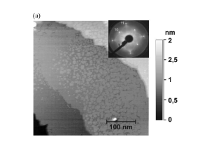
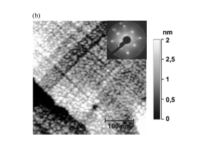
Figure 1: (a) STM image of a 10 nm thick (001)-oriented $\text{Fe}_{50}\text{Mn}_{50}\,$-layer grown on MgO(001)/Fe/Pt/Cu, the scan area is $0.4\,\mu$m$\times 0.4\,\mu$m, with a full height scale of 2 nm. The inset shows the LEED pattern of the same surface at a primary energy of 109  eV. (b) STM image of a 5 nm thick (001)-oriented $\text{Ni}_{81}\text{Fe}_{19}\,$-layer grown on top of a 10 nm thick $\text{Fe}_{50}\text{Mn}_{50}\,$-layer, the scan area is $0.4\,\mu$m$\times 0.4\,\mu$m, with a full height scale of 2 nm. The inset shows the LEED pattern of the same surface at a primary energy of 128  eV.

The magnetic properties of a $\text{Fe}_{50}\text{Mn}_{50}\,$(10  nm)/$\text{Ni}_{81}\text{Fe}_{19}\,$(5  nm) bilayer are measured using Kerr effect magnetometry. The magnetic field is applied collinear to the plane of the incident s-polarized light. The angle $\alpha_{H}$ of the in-plane [100]-direction of the $\text{Ni}_{81}\text{Fe}_{19}\,$ layer relative to the plane of the incident light is varied from 0 to 360 degree in 1 degree steps by rotating the sample. For all experimental data obtained from this rotation the decreasing field branch is shown in Fig. 2, using a magnetization reversal diagram with a grayscale proportional to the Kerr-rotation. This kind of data visualization enables the presentation of the whole angular dependence of the magnetization reversal in a single diagram and was described in detail elsewhere [28]. As can be seen in this figure the magnetization reversal diagram of the $\text{Fe}_{50}\text{Mn}_{50}\,$/$\text{Ni}_{81}\text{Fe}_{19}\,$ exchange bias system shows an asymmetry, which is characteristic for quadratic contributions to the Kerr rotation, as will be shown in the following. This asymmetry impedes a correct determination of the angular dependence of the coercive field and the exchange bias field from the raw data causing those quantities to be asymmetric with respect to the in-plane angle $\alpha_{H}$.

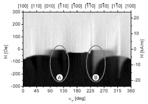
Figure 2: Magnetization reversal diagram for the branch of the hysteresis curve with decreasing external magnetic field of an epitaxial $\text{Ni}_{81}\text{Fe}_{19}\,$/$\text{Fe}_{50}\text{Mn}_{50}\,$ sample, as measured using Kerr effect magnetometry. The grayscale is proportional to the Kerr-rotation. The regions where the asymmetry discussed in the text is most obvious are marked ’A‘ and ’B‘.

The Kerr rotation $\theta_{Kerr,s}$ in longitudinal geometry with s-polarized light and the sample magnetized in the plane of the sample surface, can be written as follows [19, 32, 33, 34, 35]:

$$\theta_{Kerr,s}=\vartheta_{Kerr}^{long}M_{\|}+\vartheta_{Kerr}^{quad}M_{\|}M_{\perp},$$ (1)

where $M_{\|}$ and $M_{\perp}$ are the in-plane magnetization components parallel and perpendicular to the plane of incidence of the light. $\vartheta_{Kerr}^{long}$ and $\vartheta_{Kerr}^{quad}$ are the longitudinal and quadratic proportionality factors of the Kerr rotation. The second order term proportional to the product of the longitudinal and transverse component is the reflection analogy of the Voigt effect [29, 30, 31, 19] and gives rise to the asymmetry observed in Fig. 2. The two contributions to the Kerr rotation can be separated by making use of the symmetry of the problem as follows. As illustrated in Fig. 3, if the in-plane angle $\alpha_{H}$ of the sample with respect to the plane of the incident light is changed by 180 deg and the sign of the magnetic field $\vec{H}$ is reversed the same magnetization reversal process should be observed.

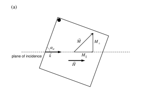
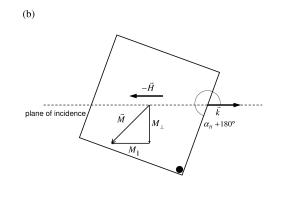
Figure 3: Geometry used to separate the different contributions to the Kerr rotation $\theta_{Kerr,s}$. (a) Situation for an angle $\alpha_{H}$ of the [100]-direction with respect to the plane of the incident light (characterized by the wavevector $\vec{k}$). (b) Equivalent situation with rotation of the sample by 180 deg and reversed direction of the applied magnetic field. The filled circle marks the orientation of the sample.

However by doing so the first term in equation (1) proportional to $M_{\|}$ changes sign while the second term proportional to $M_{\|}M_{\perp}$ will have the same sign for both sample orientations. This leads to apparently different magnetization reversal curves observed in Kerr effect magnetometry, an example of which is shown in Fig. 4 (a).

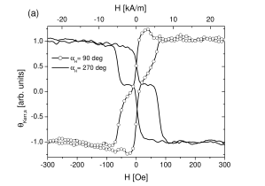
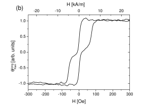
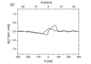
Figure 4: (a) Magnetization reversal for two equivalent angles $\alpha_{H}=90\,$deg (open symbols) and $\alpha_{H}=270\,$deg (line). Note that the sign of the magnetic field for the magnetization reversal at $\alpha_{H}=270\,$deg was reversed, so that the reversal is equivalent to that at $\alpha_{H}=90\,$deg. In (b) the linear longitudinal contribution $\theta_{Kerr}^{long}$ to the Kerr rotation of the magnetization reversal in (a) is shown, while in (c) the second-order contribution $\theta_{Kerr}^{quad}$ is shown.

By calculating the difference of the magnetization reversal for $\alpha_{H}$ and $\alpha_{H}+180\,$deg the Kerr rotation $\theta_{Kerr}^{long}$ caused by the longitudinal component of the magnetization $M_{\|}$ can be reconstructed:

$$\theta_{Kerr}^{long} := [\theta_{Kerr}(\alpha_{H})-\theta_{Kerr}(\alpha_{H}+180^{\circ})]/2$$

$$= \vartheta_{Kerr}^{long}M_{\|}.$$

This is shown in Fig. 4 (b) for the magnetization reversals shown in part (a) of the same figure. On the other hand the quadratic contribution $\theta_{Kerr}^{quad}$ to the Kerr rotation can be obtained by calculating the average of the Kerr rotation at $\alpha_{H}$ and $\alpha_{H}+180\,$deg:

$$\theta_{Kerr}^{quad} := [\theta_{Kerr}(\alpha_{H})+\theta_{Kerr}(\alpha_{H}+180^{\circ})]/2$$

$$= \vartheta_{Kerr}^{quad}M_{\|}M_{\perp},$$

as shown in Fig. 4 (c).

By carrying out the same kind of analysis for all angles $\alpha_{H}$ the magnetization reversal diagram for $\theta_{Kerr}^{long}$, i.e. for the longitudinal component of the magnetization, can be reconstructed, as is shown in Fig. 5 (a). Consequently in this figure the asymmetry that was observed in Fig. 2 is no longer present. Note however, that the symmetry breaking effect of the exchange bias effect is still visible in this diagram. A similar diagram can be constructed for the quadratic contribution $\theta_{Kerr}^{quad}$ to the Kerr rotation, as shown in Fig. 5 (b). As this diagram contains information about the product $M_{\|}M_{\perp}$ it reflects the corresponding symmetry (see also Fig. 7 (b) discussed later).

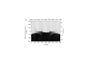
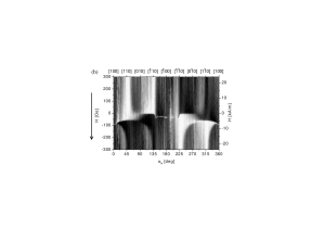
Figure 5: a) Measured magnetization reversal diagram for $\theta_{Kerr}^{long}$ caused by the longitudinal component of the magnetization $M_{\|}$. In b) the corresponding reversal diagram of the second-order contribution $\theta_{Kerr}^{quad}$ caused by $M_{\|}M_{\perp}$ is shown. In both graphs the grayscales are chosen differently in order to fit the respective data range.

The reversal data of the longitudinal component of the magnetization in Fig. 5 (a) is used to derive the angular dependence of the exchange bias field $H_{eb}$ (see Fig. 6 (a)) and the coercive field $H_{C}$ (see Fig. 6 (b)) of the $\text{Fe}_{50}\text{Mn}_{50}\,$/$\text{Ni}_{81}\text{Fe}_{19}\,$ double layer system. These angular dependencies are then fitted assuming a coherent rotation of the magnetization and using the perfect-delay convention [36] within the framework of an extended Stoner-Wohlfarth model [28, 37].

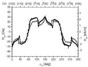
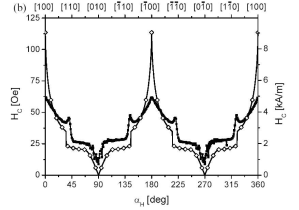
Figure 6: Angular dependence of (a) the exchange bias field and (b) the coercivity. The experimental data is shown as solid symbols, while the fit using equation III is shown as open symbols.

The experimental data can be reasonably well described by including a unidirectional anisotropy $K_{1}$ and a fourfold anisotropy $K_{4}$ contribution to Gibb’s free energy $g$ of the system, which in turn can be written as:

$$g= - K_{1}\cos(\alpha_{M})+K_{4}\sin^{2}(\alpha_{M})\cos^{2}(\alpha_{M})$$

$$- HM_{S}\cos(\alpha_{M}-\alpha_{H}).$$

A fit of the experimental data shown in Fig. 6 using the Gibb’s free energy given by equation III results in a unidirectional anisotropy $K_{1}=(2.7\pm 0.1)\,$erg/$\text{cm}^{3}$ and a fourfold anisotropy $K_{4}=(4.9\pm 0.2)\,$erg/$\text{cm}^{3}$. Note that the appearance of an induced fourfold anisotropy in addition to the unidirectional anisotropy in epitaxial $\text{Fe}_{50}\text{Mn}_{50}\,$/$\text{Ni}_{81}\text{Fe}_{19}\,$-bilayer systems has recently been shown theoretically using a vector spin model [38]. The resulting angular dependence of the exchange bias field $H_{eb}$ and the coercive field $H_{C}$ predicted by the extended Stoner-Wohlfarth model is also shown in Fig. 6.

In order to complete the picture of the magnetization reversal that results from these anisotropies within the extended Stoner-Wohlfarth model in Fig. 7 the reversal diagrams are given for both $M_{\|}$ and $M_{\|}M_{\perp}$. These two diagrams correspond to the expected linear and second-order contribution to the magneto-optic Kerr effect respectively and can therefore be directly compared with the experimental results in Fig. 5.

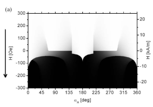
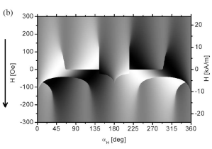
Figure 7: Magnetization reversal diagrams of the decreasing field branch, as predicted by the extended Stoner-Wohlfarth model using equation III, with $K_{1}=2.7\,$erg/$\text{cm}^{3}$ and $K_{4}=4.9\,$erg/$\text{cm}^{3}$. In a) the longitudinal component $M_{\|}$ is shown, while in b) the grayscale is proportional to the product $M_{\|}M_{\perp}$.

Given the simplification of a coherent magnetization reversal process assumed in the extended Stoner-Wohlfarth model and the small number of fitting parameters the agreement between the model and the experimental results is surprisingly good. However one notices differences between the model calculations and the experimental results especially along the axis parallel to the easy direction of the unidirectional anisotropy, i.e. around 0 deg and 180 deg. Similar deviations have been observed in epitaxial NiFe/FeMn bilayers [28] (i.e. in a system with reversed layer sequence) and may be related to thermal activation [37] or to domain formation and propagation, which are not taken into account in the Stoner-Wohlfarth model.

IV Summary

In summary we have shown that second-order magneto-optic effects are present in exchange coupled epitaxial $\text{Fe}_{50}\text{Mn}_{50}\,$/$\text{Ni}_{81}\text{Fe}_{19}\,$-bilayers. By using the method described in this article it is possible to separate the first- and second-order contributions. Thereby the asymmetry related to magneto-optics can also be separated from the one associated with the exchange bias effect. The experimental data can thus be analyzed within an extended Stoner-Wohlfarth model, which describes well the overall angular dependence of the magnetization reversal. The observed differences between the experimental data and the Stoner-Wohlfarth model may be caused by thermal activation or domain formation and propagation.

- [1] J. Kerr, Phil. Mag. 3, 321 (1877).
- [2] R.P. Cowburn, M.E. Welland, Science 287, 1466 (2000).
- [3] R.P. Cowburn, Phys. Rev. B 65, 092409 (2002)
- [4] D.A. Allwood, G. Xiong, M.D. Cooke, C.C. Faulkner, D. Atkinson, N. Vernier, R.P. Cowburn, Science 296, 2003 (2002)
- [5] D.A. Allwood, Gang Xiong, M.D. Cooke, R.P. Cowburn, J. Phys. D: Appl. Phys 36, 2175 (2003).
- [6] M.R. Freeman, M.J. Brady, J. Smyth, Appl. Phys. Lett. 60, 2555 (1992).
- [7] T.M. Crawford, T.J. Silva, C.W. Teplin, C.T. Rogers, Appl. Phys. Lett. 74, 3386 (1999).
- [8] M. Bauer, R. Lopusnik, J. Fassbender, B. Hillebrands, Appl. Phys. Lett. 76, 2758 (2000).
- [9] T.J. Silva, P. Kabos, M.R. Pufall, Appl. Phys. Lett. 81, 2205 (2002).
- [10] Ru-Pin Pan, H.D. Wei, Y.R. Shen, Phys. Rev. B 39, 1229 (1989).
- [11] W. Hübner, K.-H. Bennemann, Phys. Rev. B 40, 5973 (1989).
- [12] J. Reif, J.C. Zink, C.-M. Schneider, J. Kirschner, Phys. Rev. Lett. 67, 2878 (1991).
- [13] J. Reif, C. Rau, E. Matthias, Phys. Rev. Lett. 71, 1931 (1993).
- [14] K.H. Bennemann, Non Linear Optics in Metals, Clarendon Press, Oxford, 1998.
- [15] R.M. Osgood III, S.D. Bader, B.M. Clemens, R.L. White, H. Matsuyama, J. Magn. Magn. Mater. 182, 297 (1998).
- [16] Q.M. Zhong, A.S. Arrott, B. Heinrich, Z. Celinski, J. Appl. Phys 67, 4448 (1990).
- [17] J.A.C. Bland, M.J. Baird, H.T. Leung, A.J.R. Ives, K.D. Mackay, H.P. Hughes, J. Magn. Magn. Mater. 113, 178 (1990).
- [18] R.M. Osgood III, R.L. White, B.M. Clemens, IEEE Trans. Magn. 31, 3331 (1995).
- [19] K. Postava, H. Jaffres, A. Schuhl, F. Nguyen Van Dau, M. Goiran, A.R. Fert, J. Magn. Magn. Mater. 172, 199 (1997).
- [20] T. Ambrose, C.L. Chien, J. Appl. Phys. 83, 7222 (1998).
- [21] J. Nogués, T.J. Moran, D. Lederman, I.K. Schuller, K.V. Rao, Phys. Rev. B 59, 6984 (1999).
- [22] C. Leighton, M. Song, J. Nogués, M.C. Cyrille, I.K. Schuller, J. Appl. Phys. 88, 344 (2000).
- [23] M.R. Fitzsimmons, P. Yashar, C. Leighton, I.K. Schuller, J. Nogués, C.F. Majkrzak, J.A. Dura, Phys. Rev. Lett. 84, 3986 (2000).
- [24] M. Gierlings, M.J. Prandolini, H. Fritzsche, M. Gruyters, D. Riegel, Phys. Rev. B 65, 092407 (2002).
- [25] I.N. Krivorotov, C. Leighton, J. Nogués, I.K. Schuller, E. Dan Dahlberg, Phys. Rev. B 65, 100402 (2002).
- [26] J. McCord, R. Schäfer, R. Mattheis, K.-U. Barholz, J. Appl. Phys. 93, 5491 (2003).
- [27] T. Mewes, M. Rickart, A. Mougin, S.O. Demokritov, J. Fassbender, B. Hillebrands, M. Scheib, Surf. Sci. 481, 87 (2001).
- [28] T. Mewes, H. Nembach, M. Rickart, S.O. Demokritov, J. Fassbender, B. Hillebrands, Phys. Rev. B 65, 224423 (2002).
- [29] P.H. Lissberger, M.R. Parker, J. Appl. Phys. 42, 1708 (1971).
- [30] P.H. Lissberger, M.R. Parker, Intern. J. Magn.1, 209 (1971).
- [31] R. Carey, B.W.J. Thomas, J. Phys. D: Appl. Phys. 7, 2362 (1974).
- [32] R. Mattheis, G. Quednau, Phys. Stat. Sol. (a) 172, R7 (1999).
- [33] R. Mattheis, G. Quednau, J. Magn. Magn. Mater. 205, 143 (1999).
- [34] R. Lopusník, PhD Thesis, University Kaiserslautern (2001).
- [35] K. Postava, D. Hrabovsky, J. Pistora, A.R. Fert, S. Visnovsky, T. Yamaguchi, J. Appl. Phys 91, 7293 (2002).
- [36] S. Nieber, H. Kronmüller, phys. stat. sol. (b) 165, 503 (1991).
- [37] T. Mewes, H. Nembach, J. Fassbender, B. Hillebrands, Joo-Von Kim, R.L. Stamps, Phys. Rev. B 67, 104422 (2003).
- [38] T. Mewes, B. Hillebrands, R.L. Stamps, Phys. Rev. B, in press.