Critical Behavior of the Kramers Escape Rate in Asymmetric Classical Field Theories

Abstract

We introduce an asymmetric classical Ginzburg-Landau model in a bounded interval, and study its dynamical behavior when perturbed by weak spatiotemporal noise. The Kramers escape rate from a locally stable state is computed as a function of the interval length. An asymptotically sharp second-order phase transition in activation behavior, with corresponding critical behavior of the rate prefactor, occurs at a critical length $\ell_{c}$, similar to what is observed in symmetric models. The weak-noise exit time asymptotics, to both leading and subdominant orders, are analyzed at all interval lengthscales. The divergence of the prefactor as the critical length is approached is discussed in terms of a crossover from non-Arrhenius to Arrhenius behavior as noise intensity decreases. More general models without symmetry are observed to display similar behavior, suggesting that the presence of a “phase transition” in escape behavior is a robust and widespread phenomenon.

KEY WORDS: Fokker-Planck equation, non-Arrhenius behavior, stochastic escape problem, stochastic exit problem, stochastically perturbed dynamical systems, spatiotemporal noise, droplet nucleation, fluctuation determinant, instanton, false vacuum, stochastic Ginzburg-Landau models.

1 Introduction

Noise-induced transitions between locally stable states of spatially extended systems are responsible for a wide range of physical phenomena${}^{\footnotesize{\cite[cite]{[\@@bibref{}{GarciaOjalvo99}{}{}]}}}$. In classical systems, where the noise is typically (but not necessarily) of thermal origin, such phenomena include homogeneous nucleation of one phase inside another${}^{\footnotesize{\cite[cite]{[\@@bibref{}{Langer67}{}{}]}}}$, micromagnetic domain reversal${}^{\footnotesize{\cite[cite]{[\@@bibref{}{Braun93,Boerner98,Brown00}{}{}]}}}$, pattern nucleation in electroconvection${}^{\footnotesize{\cite[cite]{[\@@bibref{}{Bisang98andTu97}{}{}]}}}$ and other non-equilibrium systems${}^{\footnotesize{\cite[cite]{[\@@bibref{}{Cross93}{}{}]}}}$, transitions in hydrogen-bonded ferroelectrics${}^{\footnotesize{\cite[cite]{[\@@bibref{}{Dikande97}{}{}]}}}$, dislocation motion across Peierls barriers${}^{\footnotesize{\cite[cite]{[\@@bibref{}{Gorokhov97}{}{}]}}}$, instabilities of metallic nanowires${}^{\footnotesize{\cite[cite]{[\@@bibref{}{Buerkiinprep}{}{}]}}}$, and others. In quantum systems, the problem of tunneling between metastable states is formally similar, and problems of interest include decay of the false vacuum${}^{\footnotesize{\cite[cite]{[\@@bibref{}{Coleman77andCallan79}{}{}]}}}$ and metastable states in general${}^{\footnotesize{\cite[cite]{[\@@bibref{}{Affleck81}{}{}]}}}$, anomalous particle production${}^{\footnotesize{\cite[cite]{[\@@bibref{}{Frost99}{}{}]}}}$, and others.

The modern approach to these problems, beginning with the work of Langer on classical systems${}^{\footnotesize{\cite[cite]{[\@@bibref{}{Langer67}{}{}]}}}$ and Coleman and Callan on quantum systems${}^{\footnotesize{\cite[cite]{[\@@bibref{}{Coleman77andCallan79}{}{}]}}}$, considered systems of infinite spatial extent (for a review, see Schulman${}^{\footnotesize{\cite[cite]{[\@@bibref{}{Schulman81}{}{}]}}}$). In certain systems, however, finite size may lead to important modifications, and in some instances qualitatively new behavior. Approaches to noise-induced transitions between stable states in finite systems modelled by nonlinear field equations have been investigated by a number of authors${}^{\footnotesize{\cite[cite]{[\@@bibref{}{Faris82,Martinelli89,Chudnovsky92,McKane95,Kuznetsov97}{}{}]}}}$.

In a recent paper${}^{\footnotesize{\cite[cite]{[\@@bibref{}{MS01}{}{}]}}}$, Maier and Stein studied the effects of weak white noise on a bistable classical system of finite size whose zero-noise dynamics are governed by a symmetric Ginzburg-Landau $\phi^{4}$ double-well potential. Their surprising result was the uncovering of a type of second-order phase transition in activation behavior at a critical value $L_{c}$ of the system size. That a crossover in activation behavior must take place is clear from both simple physical and mathematical arguments (cf. Sec. 2). What is not so obvious is that the crossover is an asymptotically sharp, second-order phase transition in the limit of low noise. The change of behavior arises from a bifurcation of the transition state, from a zero-dimensional (i.e., constant) configuration below $L_{c}$, to a spatially varying (degenerate) pair of “periodic instantons” above $L_{c}$.

The quantitative effects of the transition are significant. In the weak-noise limit, the activation rate is given by the Kramers formula $\Gamma\sim\Gamma_{0}\exp(-\Delta W/\epsilon)$, where $\epsilon$ is the noise strength, $\Delta W$ the activation barrier, and $\Gamma_{0}$ the rate prefactor. The barrier $\Delta W$ is interpreted as the height, in dimensionless energy units, of the transition state, and by analogy with chemical kinetics, the exponential falloff of the rate is often called ‘Arrhenius behavior’. The dependence on system size $L$ of $\Delta W$ changes qualitatively at $L_{c}$. Also, the rate prefactor $\Gamma_{0}$ diverges as $L_{c}$ is approached both from above and below. Precisely at $L_{c}$, $\Gamma_{0}$ becomes $\epsilon$-dependent in such a way that it diverges as $\epsilon\to 0$. This is ‘non-Arrhenius’ behavior. (For boundary conditions that give rise to a zero mode, such as periodic, there is in addition a noise dependence of $\Gamma_{0}$ above $L_{c}$, and the prefactor divergence as $L\to L_{c}^{+}$ may be affected.)

Given the increasingly anomalous behavior of the escape rate as $L_{c}$ is approached from either side, a few words should be said about the domain of validity of the Kramers formula $\Gamma\sim\Gamma_{0}\exp(-\Delta W/\epsilon)$ for the escape rate, which displays Arrhenius behavior with both $\Gamma_{0}$ and $\Delta W$ independent of $\epsilon$. Strictly speaking, this formula is asymptotically valid, that is, only in the limit $\epsilon\to 0$. In a looser sense, the formula can often be applied to physical situations when the noise strength $\epsilon$ is both small compared to $\Delta W$, and so that the prefactor $\Gamma_{0}$ is small compared to $\exp(-\Delta W/\epsilon)$. These represent minimal requirements; in all cases applications need to be made with care. For a fuller discussion on these and related issues, see [21]. For the models presented here, a discussion of the regions of validity of all derived formulae will be presented in Sec. 4.3.

A question that naturally arises is whether this critical behavior is generic: could it depend on special features of the potential studied in [20], in particular its $\phi\to-\phi$ symmetry? It was noted${}^{\footnotesize{\cite[cite]{[\@@bibref{}{MS01}{}{}]}}}$ that in more complicated models${}^{\footnotesize{\cite[cite]{[\@@bibref{}{Kuznetsov97}{}{}]}}}$, the transition may become first-order; in others, it could conceivably disappear altogether. The purpose of this paper, however, is to provide support for the claim that the transition found in [20] is at least not confined to models with $\phi\to-\phi$ symmetry; that it should in fact appear in a wide range of models and corresponding physical situations. To support this, a nonsymmetric $\phi^{3}$ model will be studied and solved, and a second-order transition similar to that found in [20] will be uncovered. This will be followed by a brief discussion of general nonsymmetric Ginzburg-Landau models with smooth polynomial potentials up to degree four, and it will be argued that this second-order transition should appear in typical representations of these models.

2 The Model

We consider on $[-L/2,L/2]$ a classical field $\phi(x,t)$ subject to the potential

$$V(\phi)=-\alpha\phi+{1\over 3}\gamma\phi^{3}$$ (1)

as shown in Fig. 1.

Figure 1: Potential for the reduced field $u(x,t)$.

The time evolution of the field is governed by the stochastic, overdamped Ginzburg-Landau equation

$$\dot{\phi}=\kappa\phi^{\prime\prime}+\alpha-\gamma\phi^{2}+\epsilon^{1/2}\xi(x,t),$$ (2)

where $\xi(x,t)$ is white noise, satisfying $\langle\xi(x_{1},t_{1})\xi(x_{2},t_{2})\rangle=\delta(x_{1}-x_{2})\delta(t_{1}-t_{2})$. The zero-noise dynamics satisfy $\dot{\phi}=-\delta{\cal H}/\delta\phi$, with the energy functional

$${\cal H}[\phi]\equiv\int_{-L/2}^{L/2}\left[{1\over 2}\kappa(\phi^{\prime})^{2}-\alpha\phi+{1\over 3}\gamma\phi^{3}\right]\,dz.$$ (3)

Scaling out the various constants by introducing the variables $x=\Big{[}(\alpha\gamma)^{1/4}/\kappa^{1/2}\Big{]}z$, $u=\sqrt{\gamma/\alpha}\phi$, and $E_{0}=\kappa^{1/2}\alpha^{5/4}/\gamma^{3/4}$ yields

$${\cal H}[u]/E_{0}=\int_{-\ell/2}^{\ell/2}\left[{1\over 2}(u^{\prime})^{2}-u+{1\over 3}u^{3}\right]\,dx$$ (4)

where $\ell=\Big{[}(\alpha\gamma)^{1/4}/\kappa^{1/2}\Big{]}L$.

It is already clear that a crossover in activation behavior must occur. In the limit $\ell\to 0$ the gradient term in the integrand of the energy in Eq. (4) will diverge for a nonuniform state; while for $\ell\to\infty$ the $V(u)$ term will diverge for a uniform state. In this paper we will employ periodic boundary conditions throughout, and it is clear that there must be a crossover from a uniform to a nonuniform transition state as $\ell$ increases from 0. Physically, the crossover arises from a competition between the bending and bulk energies of the transition state.

This crossover will be analyzed in succeeding sections; we will see that it corresponds to an asymptotically sharp, second-order phase transition in the activation rate. Both stable and transition states are time-independent solutions of the zero-noise Ginzburg-Landau equation, that is, they are extremal states of ${\cal H}[\phi]$, satisfying

$$u^{\prime\prime}=-1+u^{2}\,.$$ (5)

As already noted, we will assume periodic boundary conditions throughout. So there is a uniform stable state $u_{s}=+1$, and a uniform unstable state $u_{u}=-1$. In the next section we will see that the latter is the transition state for $\ell<\ell_{c}=\sqrt{2}\pi$. At $\ell_{c}$ a transition occurs, and above it the transition state is nonuniform.

3 The Transition State

Following the notation of [20], we denote by $u_{{\rm inst},m}(x)$ the spatially varying, time-independent solution (“instanton state”) to the zero-noise extremum condition Eq. (5), for any $m$ in the range $0\leq m\leq 1$. The instanton state is (see Fig. 2)

$$u_{{\rm inst},m}(x,x_{0})={(2-m)\over\sqrt{m^{2}-m+1}}-{3\over\sqrt{m^{2}-m+1}}{\rm dn}^{2}\left[{x-x_{0}\over\sqrt{2}(m^{2}-m+1)^{1/4}}\Big{|}m\right]\,,$$ (6)

where dn$(\cdot|m)$ is the Jacobi elliptic function with parameter $m$, whose half-period equals ${\bf K}(m)$, the complete elliptic integral of the first kind${}^{\footnotesize{\cite[cite]{[\@@bibref{}{AS}{}{}]}}}$. Accordingly, imposition of the periodic boundary condition yields a relation between $\ell$ and $m$:

$$\ell=2\sqrt{2}(m^{2}-m+1)^{1/4}{\bf K}(m)\,.$$ (7)

Figure 2: The instanton state $u_{{\rm inst},m}(x)$ for $m=1/2$.

The minimum length that can accommodate this condition is $\ell_{c}=\sqrt{2}\pi$, corresponding to $m=0$. In this limit, ${\rm dn}(x|0)=1$, and the instanton state reduces to the uniform unstable state $u_{u}=-1$. As $m\to 1^{-}$, $\ell\to\infty$, and the instanton state becomes

$$u_{{\rm inst},1}(x)=1-3{\rm sech}^{2}\left({x-x_{0}\over\sqrt{2}}\right)\,$$ (8)

as shown in Fig. 3. As we will see, the instanton given by Eq. (6) is a saddle, or transition state, above $\ell_{c}$; it will be seen to have one unstable direction (in addition to a zero mode resulting from translational symmetry). Physically, it can be thought of as a pair of domain walls, each of which separates the two uniform states over a region of finite extent.

Figure 3: The instanton state $u_{{\rm inst},1}(x)$ on the infinite line.

For small but nonzero noise strength the leading-order asymptotics in the escape rate from the metastable well are governed by the energy difference between the transition state, which is $u_{u}=-1$ below $\ell_{c}$ and $u_{{\rm inst},m}(x)$ above, and the stable state $u_{s}=+1$. (A stability analysis justifying these identifications will be given in Secs. 4.1 and 4.2.) In the Kramers formula in Sec. 1, the activation barrier $\Delta W$, which governs exponential dependence of the escape rate on the noise strength, equals twice this energy difference. So below $\ell_{c}$, $\Delta W/2E_{0}=(4/3)\ell$. Above $\ell_{c}$, we find

$${\Delta W\over 2E_{0}}=\left({\cal H}[u_{{\rm inst},m}(x)]-{\cal H}[u_{s}=1]\right)=\left[{2-3m-3m^{2}+2m^{3}\over 3(m^{2}-m+1)^{3/2}}+{2\over 3}\right]\ell$$ (9)

$$+{12\sqrt{2}\over 5(m^{2}-m+1)^{1/4}}\left[2{\bf E}(m)-{(2-m)(1-m)\over(m^{2}-m+1)}{\bf K}(m)\right]\,,$$ (10)

where ${\bf E}(m)$ is the complete elliptic integral of the second kind${}^{\footnotesize{\cite[cite]{[\@@bibref{}{AS}{}{}]}}}$. The activation barrier for the entire range of $\ell$ is shown in Fig. 4. As $\ell\to\infty$, $\Delta W/2E_{0}\to 24\sqrt{2}/5$; this value is simply the energy of a pair of domain walls.

Figure 4: The activation barrier $\Delta W/2E_{0}$ for periodic boundary conditions (solid line). The dashed line indicates the crossover from the uniform transition state to the instanton transition state at $\ell_{c}$, and the dotted line an extension to the region $\ell>\ell_{c}$ of the activation energy corresponding to the uniform state.

4 Rate prefactor

For an overdamped multidimensional system driven by white noise, the rate prefactor $\Gamma_{0}$ can be computed as follows${}^{\footnotesize{\cite[cite]{[\@@bibref{}{HTB90,MM}{}{}]}}}$ (see also [2, 14]). As in [20], let ${\bf\varphi}_{s}$ denote the stable state, and let ${\bf\varphi}_{u}$ denote the transition state; it will be assumed (as is the case here) that this state has a single unstable direction. Consider a small perturbation ${\bf\eta}$ about the stable state, i.e., ${\bf\varphi}={\bf\varphi}_{s}+{\bf\eta}$. Then to leading order $\dot{\bf\eta}=-{\bf\Lambda}_{s}{\bf\eta}$, where ${\bf\Lambda}_{s}$ is the linearized zero-noise dynamics at ${\bf\varphi}_{s}$. Similarly ${\bf\Lambda}_{u}$ is the linearized zero-noise dynamics around ${\bf\varphi}_{u}$. Then${}^{\footnotesize{\cite[cite]{[\@@bibref{}{HTB90,MM}{}{}]}}}$

$$\Gamma_{0}=\frac{1}{2\pi}\sqrt{\left|\frac{\det{\bf\Lambda}_{s}}{\det{\bf\Lambda}_{u}}\right|}\,\,\left|\lambda_{u,1}\right|,$$ (11)

where $\lambda_{u,1}$ is the only negative eigenvalue of ${\bf\Lambda}_{u}$, corresponding to the direction along which the optimal escape trajectory approaches the transition state. In general, the determinants in the numerator and denominator of Eq. (11) separately diverge: they are products of an infinite number of eigenvalues with magnitude greater than one. However, their ratio, which can be interpreted as the limit of a product of individual eigenvalue quotients, is finite.

4.1 $\ell<\ell_{c}$

In this regime, both the stable and transition states are uniform, allowing for a straightforward determination of $\Gamma_{0}$ by direct computation of the determinants. Using reduced variables, the stable state $u_{s}=+1$ and the transition state $u_{u}=-1$. Linearizing around the stable state gives

$$\dot{\eta}=-\hat{\Lambda}[u_{s}]\eta=-(-d^{2}/dx^{2}+2)\eta\,,$$ (12)

and similarly

$$\dot{\eta}=-\hat{\Lambda}[u_{u}]\eta=-(-d^{2}/dx^{2}-2)\eta\,$$ (13)

about the transition state. The spectrum of eigenvalues corresponding to $\hat{\Lambda}[u_{s}]$ is

$$\lambda_{n}^{s}=2+{4\pi^{2}n^{2}\over\ell^{2}}\qquad\qquad\qquad n=0,\pm 1,\pm 2\ldots$$ (14)

and the eigenvalues corresponding to $\hat{\Lambda}[u_{u}]$ are

$$\lambda_{n}^{u}=-2+{4\pi^{2}n^{2}\over\ell^{2}}\qquad\qquad\qquad n=0,\pm 1,\pm 2\ldots\,.$$ (15)

This simple linear stability analysis justifies the claims that $u_{s}$ is a stable state and $u_{u}$ a transition state, or saddle point. Over the interval $[0,\ell_{c})$ all eigenvalues of $\hat{\Lambda}[u_{s}]$ are positive, while all but one of $\hat{\Lambda}[u_{u}]$ are. Its single negative eigenvalue $\lambda_{0}^{u}=-2$ is independent of $\ell$, and the corresponding eigenfunction, which is spatially uniform, is the direction in configuration space along which the optimal escape path approaches $u_{u}$.

Putting everything together, we find

$$\Gamma_{0} = {1\over\pi}\sqrt{\left|{\prod_{n=-\infty}^{\infty}(2+{4\pi^{2}n^{2}\over\ell^{2}})\over\prod_{n=-\infty}^{\infty}(-2+{4\pi^{2}n^{2}\over\ell^{2}})}\right|}$$ (16)

$$= {1\over\pi}{\sinh(\ell/\sqrt{2})\over\sin(\ell/\sqrt{2})}\,,$$

which diverges at $l_{c}=\sqrt{2}\pi$ as expected; in this limit, $\Gamma_{0}\sim{\rm const}\times(\ell_{c}-l)^{-1}$. The divergence arises from the vanishing of the pair of eigenvalues $\lambda^{u}_{\pm 1}$ as $\ell\to\ell_{c}^{-}$ (each eigenvalue contributing a factor $(\ell_{c}-\ell)^{-1/2}$). This indicates the appearance of a pair of soft modes, resulting in a transversal instability of the optimal escape trajectory as the saddle point is approached.

4.2 $\ell>\ell_{c}$

Computation of the determinant quotient in Eq. (11) is less straightforward when the transition state is nonconstant. This occurs when $\ell>\ell_{c}$, where the transition state $u_{u}$ is given by Eq. (6), and its associated linearized evolution operator is

$$\hat{\Lambda}[u_{u}]=-{d^{2}\over dx^{2}}+{2(2-m)\over\sqrt{m^{2}-m+1}}-{6\over\sqrt{m^{2}-m+1}}\ {\rm dn}^{2}\left[{x-x_{0}\over\sqrt{2}(m^{2}-m+1)^{1/4}}\Big{|}m\right]\,.$$ (17)

Evaluation of $\Gamma_{0}$ therefore requires determination of the eigenvalue spectrum of $\hat{\Lambda}[u_{u}]$ with periodic boundary conditions.

An additional complication follows from the infinite translational degeneracy of the instanton state (i.e., invariance with respect to choice of $x_{0}$). This implies a soft collective mode in the linearized dynamical operator $\hat{\Lambda}[u_{u}]$ of Eq. (17), resulting in a zero eigenvalue. Removal of this zero eigenvalue can be achieved with the McKane-Tarlie regularization procedure${}^{\footnotesize{\cite[cite]{[\@@bibref{}{McKane95}{}{}]}}}$ for functional determinants.

That procedure is implemented as follows (see [18] for details). Let $y_{1}(x,x_{0};m)$ and $y_{2}(x,x_{0};m)$ denote two linearly independent solutions of $\hat{\Lambda}[u_{u}]y_{i}=0$, $i=1,2$. Let $\det^{\prime}\hat{\Lambda}$ refer to the functional determinant of the operator $\hat{\Lambda}$ with the zero eigenvalue removed. Then, with periodic boundary conditions, it is formally the case that

$${\det^{\prime}\hat{\Lambda}\over\langle y_{1}|y_{1}\rangle}={y_{2}(z+\ell)-y_{2}(z)\over y_{1}(z)\det{\bf H}(z)}$$ (18)

where $z$ is arbitrary, $\langle y_{1}|y_{1}\rangle=\int_{-\ell/2}^{\ell/2}dx\ y_{1}^{2}(x,0;m)$ is the square of the norm of the zero mode and $\det{\bf H}(z)=\dot{y}_{2}(z)y_{1}(z)-\dot{y}_{1}(z)y_{2}(z)$ is the Wronskian. (The expression (18) is meaningful only as part of a determinant quotient; see below.)

Solutions $y_{1}$ and $y_{2}$ of $\hat{\Lambda}[u_{u}]y_{i}=0$ can be found by differentiating the instanton solution (6) with respect to $x_{0}$ and $m$, respectively; i.e., $y_{1}(x,x_{0};m)=\partial u_{{\rm inst},m}(x,x_{0};m)/\partial x_{0}$ and $y_{2}(x,x_{0};m)=\partial u_{{\rm inst},m}(x,x_{0};m)/\partial m$. The homogeneous solutions are then

$$y_{1}(x,x_{0};m)=-{6m\beta(m)^{3}\over\sqrt{2}}{\rm sn}\left[{\beta(m)(x-x_{0})\over\sqrt{2}}\Big{|}m\right]{\rm cn}\left[{\beta(m)(x-x_{0})\over\sqrt{2}}\Big{|}m\right]{\rm dn}\left[{\beta(m)(x-x_{0})\over\sqrt{2}}\Big{|}m\right]$$ (19)

and

$$y_{2}(x,x_{0};m) = -{3m\beta(m)^{6}\over 2}+{3\beta(m)^{2}\over(1-m)}{\rm sn}^{2}\left[{\beta(m)(x-x_{0})\over\sqrt{2}}\Big{|}m\right]{\rm dn}^{2}\left[{\beta(m)(x-x_{0})\over\sqrt{2}}\Big{|}m\right]$$ (20)

$$+ {3(2m-1)\beta(m)^{6}\over 2}{\rm dn}^{2}\left[{\beta(m)(x-x_{0})\over\sqrt{2}}\Big{|}m\right]$$

$$+ 3\beta(m)^{2}{\rm sn}\left[{\beta(m)(x-x_{0})\over\sqrt{2}}\Big{|}m\right]{\rm cn}\left[{\beta(m)(x-x_{0})\over\sqrt{2}}\Big{|}m\right]{\rm dn}\left[{\beta(m)(x-x_{0})\over\sqrt{2}}\Big{|}m\right]$$

$$\times \left\{{(2-m)\beta(m)^{5}(x-x_{0})\over 2\sqrt{2}}-{{\bf E}\left({\beta(m)(x-x_{0})\over\sqrt{2}}\Big{|}m\right)\over 1-m}\right\}\,,$$

where $\beta(m)=(m^{2}-m+1)^{-1/4}$ and ${\bf E}(\cdot|m)$ is the incomplete elliptic integral of the second kind${}^{\footnotesize{\cite[cite]{[\@@bibref{}{AS}{}{}]}}}$. Inserting these solutions into Eq. (18) yields

$$\left|{\det^{\prime}\hat{\Lambda}[u_{u}]\over\langle y_{1}|y_{1}\rangle}\right|={(m^{2}-m+1)^{11/4}\over 9m^{2}(1-m)}\left[{2{\bf E}(m)\over 1-m}-{(2-m){\bf K}(m)\over m^{2}-m+1}\right]\,.$$ (21)

Using a similar procedure (see the Appendix of [18]), we find the corresponding numerator for the determinant ratio in Eq. (11) to be

$$\det\hat{\Lambda}[u_{s}]=4\sinh^{2}(\ell/\sqrt{2})\,,$$ (22)

consistent with the numerator of Eq. (16), obtained through direct computation of the eigenvalue spectrum. We emphasize again, however (cf. the discussion above Eq. (16)), that it is only the ratio of the determinants that is sensible, not the individual determinants themselves: these each diverge for every $\ell$. In contrast, the expressions in Eqs. (21) and (22) are well-behaved for all finite $\ell>\ell_{c}$ ($m>0$), but still separately diverge in the $\ell\to\infty$ ($m\to 1$) limit. Nevertheless, here also the divergences cancel to give

$$\lim_{m\to 1}\sqrt{\left|{\det\hat{\Lambda}[u_{s}]\over\det^{\prime}\hat{\Lambda}[u_{u}]}\right|}=24\sqrt{2}\Big{/}\sqrt{\langle y_{1}|y_{1}\rangle}\,.$$ (23)

We next compute the eigenvalue $\lambda_{u,1}$ corresponding to the unstable direction. With the substitution $w=\beta(m)(x-x_{0})/\sqrt{2}$, the eigenvalue equation $\hat{\Lambda}[u_{u}]\eta=\lambda\eta$ becomes

$$d^{2}\eta/dw^{2}+12{\rm dn}^{2}[w|m]\eta={\cal E}\eta$$ (24)

where ${\cal E}=-2\lambda/\beta(m)^{2}+4(2-m)$. Using the identity${}^{\footnotesize{\cite[cite]{[\@@bibref{}{AS}{}{}]}}}$ ${\rm dn}^{2}[z|m]=1-m{\rm sn}^{2}[z|m]$, we observe that Eq. (24) is the $l=3$ Lamé equation${}^{\footnotesize{\cite[cite]{[\@@bibref{}{WW27,LK00}{}{}]}}}$, a Schrödinger equation with periodic potential of period $2{\bf K}(m)$. Its Bloch wave spectrum consists of four energy bands, and its eigenfunctions can be expressed in terms of Lamé polynomials${}^{\footnotesize{\cite[cite]{[\@@bibref{}{WW27}{}{}]}}}$. A fuller discussion, especially for higher $l$-values, is given in [26]; for our purposes here we do not need to utilize the full machinery of the Hermite solution (a detailed treatment is given in [24]).

It is easy to check that the eigenvector $\eta_{u_{1}}$ with smallest eigenvalue is

$$\eta_{u,1}(x,x_{0};m)={\rm dn}^{3}\left[{\beta(m)(x-x_{0})\over\sqrt{2}}\Big{|}m\right]+C(m){\rm dn}\left[{\beta(m)(x-x_{0})\over\sqrt{2}}\Big{|}m\right]\,$$ (25)

where $C(m)=-[2(2-m)/5]+(1/5)\sqrt{4m^{2}-m+1}$, and

$$\lambda_{u,1}=-\left[{1\over 2}(2-m)+\sqrt{4m^{2}-m+1}\right]\beta(m)^{2}\,,$$ (26)

which approaches $-2$ as $m\to 0$ in agreement with the single negative eigenvalue of Eq. (15).

As noted in [20], the full translational symmetry of the periodic instanton state in the periodic boundary condition case corresponds to a ‘soft mode’, resulting in appearance of a zero eigenvalue $\lambda_{u,2}=0$ of the operator $\hat{\Lambda}[u_{u}]$. (The corresponding eigenfunction $\eta_{u,2}$ is given by $y_{1}$ in Eq. (19).) Physically, this corresponds to zero translational energy of the instanton; i.e., it can appear anywhere in the volume (in contrast with, say, Dirichlet boundary conditions, where the instanton is ‘pinned’.) This should result in an overall factor of $\ell$, indicating that the physical quantity of interest above $\ell_{c}$ is the transition rate per unit length. The general procedure for including this correction is described by Schulman [14]. (Our case differs by a factor of 2 from his due to the lack of symmetry in our model.) The net result is to multiply the prefactor by

$$\zeta=\ell\langle y_{1}|y_{1}\rangle^{1/2}/\sqrt{\pi\epsilon}\,.$$ (27)

The most important qualitative changes are the $\epsilon^{-1/2}$ factor, leading to a non-Arrhenius transition rate above $\ell_{c}$, and the effect on the behavior as $\ell\to\ell_{c}^{+}$; both will be discussed in more detail below.

The above discussion also makes clear that it is not necessary to separately evaluate $\langle y_{1}|y_{1}\rangle$. For completeness’ sake, however, we present it as well. Its evaluation is straightforward and yields

$$\langle y_{1}|y_{1}\rangle={72\sqrt{2}\beta(m)\over 15}{\bf E}(m)-{36\sqrt{2}\beta(m)^{5}(m^{2}-3m+2)\over 15}{\bf K}(m)$$ (28)

which equals $24\sqrt{2}/5$ in the $m\to 1$ limit.

Putting everything together, we find the rate per unit length prefactor for $\ell>\ell_{c}$ to be

$$\Gamma_{0}/\ell = {\epsilon^{-1/2}\over\pi^{3/2}}{3m(1-m)\over(m^{2}-m+1)^{11/8}}\left[{1\over 2}(2-m)+\sqrt{4m^{2}-m+1}\right]$$ (29)

$$\times \sqrt{\sinh^{2}\left(2(m^{2}-m+1)^{1/4}{\bf K}(m)\right)\over 2(m^{2}-m+1){\bf E}(m)-(2-m)(1-m){\bf K}(m)}\,.$$

The prefactor over the entire range of $\ell$ is plotted in Fig. 5. The prefactor divergence has a critical exponent of 1 as $\ell\to\ell_{c}^{-}$. Above $\ell_{c}$ the prefactor is non-Arrhenius everywhere, and the vertical axis is rescaled to account for the singular $\epsilon^{1/2}$ behavior.

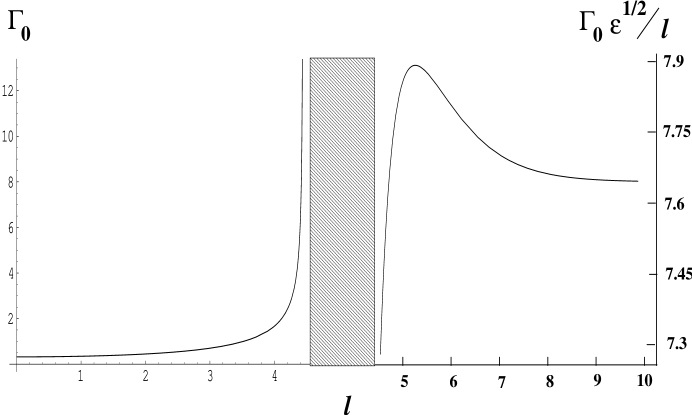
Figure 5: The Kramers rate prefactor $\Gamma_{0}$. Because of the qualitative change in behavior, from Arrhenius to non-Arrhenius, at $\ell_{c}$, different vertical scales are used below and above the transition.

The rescaled prefactor above $\ell_{c}$ as a function of $m$ is shown in Fig. 6, in order to indicate more clearly the $m\to 0$ ($\ell\to\ell_{c}$) behavior.

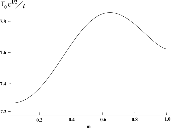
Figure 6: The Kramers rate prefactor $\Gamma_{0}$ per unit length above $\ell_{c}$.

The behavior of the rate prefactor $\Gamma_{0}$ for all $\ell>\ell_{c}$ is unusual in two ways. First, it is non-Arrhenius — that is, it scales as $\epsilon^{-1/2}$ for all $\epsilon\to 0$. Second, it does not formally diverge as $\ell\to\ell_{c}^{+}$, as seen in Fig. 6 (in fact, the divergence is present but ‘masked’, as discussed below). Both of these features are consequences of the translation-invariance of the periodic boundary conditions used here, and would not appear if translation-noninvariant boundary conditions, such as Dirichlet or Neumann, are used. (See, for example, Fig. 3 of [20].)

Such boundary condition-dependent behavior should be distinguished from the boundary condition-independent formal divergence of the prefactor as the critical length is approached, as explained below, and of the non-Arrhenius behavior (to be discussed in Sec. 4.3 below) exactly at the critical length. By boundary condition-independent, we mean behavior that is seen in all four of the most commonly used boundary conditions in this type of problem, namely periodic, antiperiodic, Dirichlet, and Neumann; all were considered for symmetric quartic potentials in [27]. In the present case of periodic boundary conditions, the removal of the zero mode that is present for all $\ell>\ell_{c}$ renormalizes the prefactor by the factor $\zeta$ in Eq. (27). This renormalization masks the divergence of the determinant ratio as $\ell\to\ell_{c}^{+}$, because the factor $\zeta$ includes the Jacobian of the transformation${}^{\footnotesize{\cite[cite]{[\@@bibref{}{Schulman81}{}{}]}}}$ from the translation-invariant normal mode to the variable $x_{0}$; this in turn equals the norm $\sqrt{\langle y_{1}|y_{1}\rangle}$, which vanishes as $m\to 0$. The crucial point is that a divergence is still embedded within the prefactor, in the sense that the square root of the determinant ratio diverges with a critical exponent of $1/2$ as $\ell\to\ell_{c}^{+}$. Upon closer examination, this arises from the lowest stable eigenvalue, $\lambda_{u,3}$, of $\det\Lambda^{\prime}[u_{u}]$ approaching zero as $\ell\to\ell_{c}^{+}$, in a similar fashion to the eigenvalue behavior below $\ell_{c}$ (cf. $n=\pm 1$ in Eq. (15)). This eigenvalue and its corresponding eigenfunction $\eta_{u,3}$ are given by

$$\eta_{u,3}(x,x_{0};m)={\rm dn}^{3}\left[{\beta(m)(x-x_{0})\over\sqrt{2}}\Big{|}m\right]+C^{\prime}(m){\rm dn}\left[{\beta(m)(x-x_{0})\over\sqrt{2}}\Big{|}m\right]\,$$ (30)

where $C^{\prime}(m)=-[2(2-m)/5+(1/5)\sqrt{4m^{2}-m+1}]$, and

$$\lambda_{u,3}=-\left[{1\over 2}(2-m)-\sqrt{4m^{2}-m+1}\right]\beta(m)^{2}\,.$$ (31)

Fig. 7 shows the lowest three eigenvalues for the operators $\hat{\Lambda}[u_{u}^{<}]$ and $\hat{\Lambda}[u_{u}^{>}]$, where $u_{u}^{<}$ ($u_{u}^{>}$) indicates the transition state below (above) $\ell_{c}$. This figure illustrates the evolution of the eigenvalues ($\lambda_{\pm 1}^{<}$ and $\lambda_{3}^{>}$) that control the formal prefactor divergence as $\ell$ passes through $\ell_{c}$. We note in particular the merging of the second and third eigenvalues of $\hat{\Lambda}[u_{u}^{>}]$ as $\ell\to\ell_{c}^{+}$, consistent with the double degeneracy of the corresponding eigenfunction when $\ell<\ell_{c}$. The eigenvalues are everywhere continuous. Fig. 8 displays the behavior of the full determinant ratio above $\ell_{c}$.

Figure 7: Behavior of the lowest three eigenvalues of the operators $\hat{\Lambda}[u_{u}^{<}]$ and $\hat{\Lambda}[u_{u}^{>}]$. The vertical dashed line is $\ell=\ell_{c}$. The eigenvalues $\lambda_{n}^{<}$ correspond to $n=0,\pm 1$ of Eq. (15). Computation of the three lowest eigenvalues $\lambda_{1,2,3}^{>}$ in the $\ell>\ell_{c}$ region is given in the text. The bold curve corresponding to $\lambda_{\pm 1}^{<}$ reflects its double degeneracy.

Figure 8: Behavior of the ratio of the eigenvalue spectrum above $\ell_{c}$.

4.3 Interpretation of the Prefactor Divergence

The formal divergence of the Kramers rate prefactor at a critical length $l_{c}$ (cf. Fig. 5) requires interpretation. It is interesting that a prefactor divergence was also found${}^{\footnotesize{\cite[cite]{[\@@bibref{}{MS93,MS96}{}{}]}}}$ in a completely different set of systems, namely spatially homogeneous (i.e., zero-dimensional) systems out of equilibrium, i.e., in which detailed balance is not satisfied in the stationary state. That divergence arose from an entirely different reason: the appearance of a caustic singularity in the vicinity of the most probable exit path as a parameter in the drift field varied. The caustic singularity arises from the unfolding of a boundary catastrophe; a detailed analysis in given in [31]. In contrast, the problem considered here is that of a spatially extended system in equilibrium, so no such singularities can be present. Moreover, no parameter in the stochastic differential equations describing the time evolution of the system is being varied in the case under discussion here; rather, the variation is in the length of the interval on which the field is defined. The ‘phase transitions’ in the stochastic exit problem in the two classes of systems are therefore physically unrelated.

What does it mean for the prefactor to (formally) diverge? In fact, at no lengthscale is the true prefactor infinite, for any $\epsilon>0$. Indeed, given that the analysis presented here is, strictly speaking, valid only asymptotically as $\epsilon\to 0$, the escape rate is always small where the above results are applicable. What the formal divergence of the prefactor does mean is that the escape behavior becomes increasingly anomalous as $\ell_{c}$ is approached, and it is asymptotically non-Arrhenius exactly at $\ell_{c}$.

That is, when $\ell=\ell_{c}$ the true rate prefactor should scale as a (negative) power of $\epsilon$ for all $\epsilon\to 0$. As in [28, 29], this can be treated quantitatively by studying the ’splayout’ of the ‘tube’ within which fluctuations are largely confined, as the saddle is approached. ‘Splayout’ here simply means that the fluctuational tube width, which for $\ell\neq\ell_{c}$ is $O(\epsilon^{1/2})$, becomes $O(\epsilon^{\alpha})$, with $\alpha<1/2$, as the saddle is approached when $\ell=\ell_{c}$. In the model studied in [28, 29], the Lagrangian manifold comprising optimal fluctuational trajectories has a more complicated behavior than in the model under study here. As a result, in [28, 29] fluctuations near the saddle occur on all lengthscales, while in the present case fluctuations near the saddle occur on a definite lengthscale, but one larger than $O(\epsilon^{1/2})$, leading to non-Arrhenius behavior for all $\epsilon\to 0$. Details will be presented in [30].

Our main interest here is in the region close to $\ell_{c}$, where the rate prefactor $\Gamma_{0}$ is growing anomalously large (but remains everywhere finite for all $\ell$ strictly away from $\ell_{c}$). The formulas given here are valid for $\epsilon$ sufficiently small so that the contribution from the quadratic fluctuations about the relevant extremal state of ${\cal H}[\phi]$ dominates the action. As long as all eigenvalues of $\hat{\Lambda}[u_{u}]$ are nonzero (excluding the zero mode arising from translational symmetry, which may be extracted), and the norms of the corresponding eigenfunctions are bounded away from zero, the prefactor formula applies, but in an $\epsilon$-region driven to zero as $\ell\to\ell_{c}$ by the rate of vanishing of the eigenvalue(s) of smallest magnitude. Therefore, as $\ell\to\ell_{c}$ from either side, the Kramers rate formula applies when $\epsilon$ scales to zero at least as fast as $|\ell-\ell_{c}|^{1/2}$ (of course, the constraints already mentioned in Sec. 1 must continue to hold as well). More precisely, the criterion considered here (which is necessary but not a priori sufficient) for Arrhenius behavior to hold on either side of $\ell_{c}$ is that the noise strength $\epsilon$ be small compared to $\lambda_{m}\langle\eta_{m}|\eta_{m}\rangle$, where $\lambda_{m}$ is the eigenvalue of smallest magnitude and $\eta_{m}$ its corresponding eigenfunction(s). This criterion arises from the condition, used in the derivation of Eq. (11), that the noise strength be small compared to the size of quadratic fluctuations about the extremal action. For $\ell$ slightly below $\ell_{c}$, these quantities are given in Sec. 4.1, and above $\ell_{c}$, by Eqs. (30) and (31). The resulting computation is straightforward and the resulting $\epsilon$-region is sketched in Fig. 9 (in the dimensionless units used here, the coefficients of the scaling terms are of $O(1)$).

Figure 9: A sketch of the scaling of the regions where the Arrhenius prefactor formulae given by Eqs. (16) and (29) are valid, when $\ell$ is very close to $\ell_{c}$. For fixed $\ell$, $\epsilon$ must be small enough so that it is below the shaded region for these formulae to apply. Non-Arrhenius behavior is expected in the shaded region. Because this figure is intended to illustrate only the rate of scaling of $\epsilon$ with $|l-l_{c}|$ so that the Kramers rate formula is valid, the axes are unmarked (except for $\ell=\ell_{c}$, where the $\epsilon$-range has shrunk to zero).

The result is that, for fixed $\ell$ close to $\ell_{c}$, there should be a crossover from non-Arrhenius to Arrhenius behavior at sufficiently weak noise strength (cf. [29]). The figure represents a type of ‘Ginzburg criterion’ that describes, at a given $\ell$ near $\ell_{c}$, how far down as $\epsilon\to 0$ the non-Arrhenius behavior persists. It should be emphasized that Fig. 9 sets an upper bound on the scaling of the region of $\epsilon$ vs. $|\ell-\ell_{c}|$, below which asymptotic Arrhenius behavior sets in. It would be interesting to consider also the behavior at very small but fixed noise as $\ell$ increases thorugh $\ell_{c}$. Here one would observe a crossover from Arrhenius to non-Arrhenius behavior and back again as $\ell$ passes through the critical region. An interesting problem for future consideration is to analyze this phenomenon in greater quantitative detail.

To summarize: strictly away from $\ell_{c}$, the prefactor formulae Eqs. (16) and (29) hold (corresponding to Arrhenius behavior of the rate), but in an increasingly narrow range of $\epsilon$ as $\ell_{c}$ is approached. A crossover from non-Arrhenius to Arrhenius behavior as $\epsilon\to 0$ should be observed, along a boundary that scales as shown in Fig. 9. Strictly at $\ell_{c}$, the formulae do not hold: the prefactor is finite, but acquires a power-law (in $\epsilon$) character. That is, the rate behavior is non-Arrhenius all the way down to $\epsilon\to 0$. This (boundary condition-independent) non-Arrhenius behavior at criticality should be distinguished from the (noncritical) non-Arrhenius behavior strictly above $\ell_{c}$ that appears only when translation-invariant boundary conditions, such as periodic, are used.

5 Asymmetric quartic potentials

In this section we will consider more general asymmetric potentials of the form

$$V(u)=-(1/2)u^{2}-(1/3)u^{3}+(1/4)u^{4}$$ (32)

as shown in Fig. 10.

Figure 10: The asymmetric quartic potential of Eq. (32).

We will consider only the small-$\ell$ regime, and show that a transition at finite $\ell_{c}$ exists with a divergence of the prefactor as $\ell\to\ell_{c}$.

Because the prefactor depends on the curvature of the potential near its minimum, different prefactors (and of course activation energies) correspond to the two minima $u_{-}=1/2-\sqrt{5}/2\approx-.62$ and $u_{+}=1/2+\sqrt{5}/2\approx 1.62$. The formulae shown here correspond to $u_{-}$; corresponding formulae for escape from the potential minimum from $u_{+}$ are obtained by replacing the constant $a_{-}=|1+2u_{-}-3u_{-}^{2}|\approx 1.38$ with $a_{+}=|1+2u_{+}-3u_{+}^{2}|\approx 3.62$. The critical length $\ell_{c}$ is the same in the two cases.

An analysis similar to that of Sec. 4.1 yields

$$\Gamma_{0}={(a_{-})^{1/4}\over 2\pi}{\sinh(a_{-}\ell/2)\over\sin(\ell/2)}$$ (33)

so $\ell_{c}=2\pi$ and, as before, the prefactor again diverges as $(1-\ell/\ell_{c})^{-1}$ as $\ell\to\ell_{c}^{-}$, as shown in Fig. 11.

Figure 11: The prefactor $\Gamma_{0}$ of Eq. (33) for $\ell<\ell_{c}$.

6 Conclusion

We have found an explicit solution of the Kramers escape rate in an asymmetric $\phi^{3}$ field theory of the Ginzburg-Landau form. This result, and the brief discussion in Sec. 5 of more general asymmetric potentials, suggests that the critical behavior found in [20] might hold for a more general class of models than those with a high degree of symmetry. How widespread the transition phenomenon is remains uncertain, but it appears to hold at least for arbitrary smooth potentials with terms up to and including $\phi^{4}$. It would be interesting to find models with other types of behaviors. One interesting possibility, discussed in [20], is a class of models that display a first-order transition: for example, a discontinuity in the derivative of the activation barrier height with respect to the interval length, at a critical length. A possible candidate for such a model is the sixth-degree Ginzburg-Landau potential of Kuznetsov and Tinyakov [19], but a detailed analysis of its transition behavior remains to be done.

Acknowledgment. I would like to thank Robert Maier for useful comments on the manuscript, and for many valuable discussions.

References

- [1] J. García-Ojalvo and J. M. Sancho, Noise in Spatially Extended Systems (Springer, New York/Berlin, 1999).
- [2] J. S. Langer, Ann. Physics 41, 108 (1967). See also M. Büttiker and R. Landauer, Phys. Rev. Lett. 43, 1453 (1979); Phys. Rev. A 23, 1397 (1981).
- [3] H.-B. Braun, Phys. Rev. Lett. 71, 3557 (1993).
- [4] E. D. Boerner and H. N. Bertram, IEEE Trans. Magnetics 34, 1678 (1998).
- [5] G. Brown, M. A. Novotny, and P. A. Rikvold, J. Appl. Phys. 87, 4792 (2000).
- [6] U. Bisang and G. Ahlers, Phys. Rev. Lett. 80, 3061 (1998); Y. Tu, Phys. Rev. E 56, R3765 (1997).
- [7] M.C. Cross and P.C. Hohenberg, Rev. Mod. Phys. 65, 851 (1993).
- [8] A.M. Dikandé, ICTP preprint IC9730 (1997).
- [9] D.A. Gorokhov and G. Blatter, Phys. Rev. B 56, 3130 (1997). The authors find a crossover from a classical, thermally activated regime to a quantum tunneling regime.
- [10] J. Buerki, C. Stafford, and D.L. Stein, in preparation.
- [11] S. Coleman, Phys. Rev. D 15, 2929 (1977); C.G. Callan, Jr. and S. Coleman, Phys. Rev. D 16, 1762 (1977).
- [12] I. Affleck, Phys. Rev. Lett. 46, 388 (1981). Crossover from classical activation to quantum tunneling is considered here also.
- [13] K.L. Frost and L.G. Yaffe, Phys. Rev. D 59, 065013-1 (1999).
- [14] L.S. Schulman, Techniques and Applications of Path Integration (Wiley, New York, 1981), chapter 29.
- [15] W. G. Faris and G. Jona-Lasinio, J. Phys. A 15, 3025 (1982).
- [16] F. Martinelli, E. Olivieri, and E. Scoppola, J. Stat. Phys. 55, 477 (1989).
- [17] E. M. Chudnovsky, Phys. Rev. A 46, 8011 (1992).
- [18] A.J. McKane and M.B. Tarlie, J. Phys. A 28, 6931 (1995).
- [19] A.N. Kuznetsov and P.G. Tinyakov, Phys. Lett. B 406, 76 (1997).
- [20] R.S. Maier and D.L. Stein, Phys. Rev. Lett. 87, 270601-1 (2001).
- [21] P. Hänggi, P. Talkner, and M. Borkovec, Rev. Mod. Phys. 62, 251 (1990).
- [22] Handbook of Mathematical Functions, edited by M. Abramowitz and I. A. Stegun (Dover, New York, 1965).
- [23] Theory of Continuous Fokker–Planck Systems, edited by F. Moss and P. V. E. McClintock (Cambridge University Press, Cambridge, 1989).
- [24] E.T. Whittaker and G.N. Watson, A Course of Modern Analysis (Cambridge University Press, Cambridge, 1927), 4th ed.,Sec. 23.71.
- [25] H. Li and D. Kusnezov, Phys. Rev. Lett. 83, 1283 (2000).
- [26] R.S. Maier, “Lamé Polynomials, the Lamé Dispersion Relation, and Hyperelliptic Reduction”, in preparation.
- [27] R.S. Maier and D.L. Stein, in Noise in Complex Systems and Stochastic Dynamics, eds. L. Schimansky-Geier, D. Abbott, A. Neiman, and C. Van den Broeck (SPIE Proceedings Series, v. 5114, 2003), pp. 67–78.
- [28] R.S. Maier and D.L. Stein, Phys. Rev. Lett. 71, 1783 (1993).
- [29] R.S. Maier and D.L. Stein, J. Stat. Phys. 83, 291 (1996).
- [30] R.S. Maier and D.L. Stein, in preparation.
- [31] R.S. Maier and D.L. Stein, Phys. Rev. Lett. 85, 1358 (2000).