Thermalization of an anisotropic granular particle

Abstract

We investigate the dynamics of a needle in a two-dimensional bath composed of thermalized point particles. Collisions between the needle and points are inelastic and characterized by a normal restitution coefficient $\alpha<1$. By using the Enskog-Boltzmann equation, we obtain analytical expressions for the translational and rotational granular temperatures of the needle and show that these are, in general, different from the bath temperature. The translational temperature always exceeds the rotational one, though the difference decreases with increasing moment of inertia. The predictions of the theory are in very good agreement with numerical simulations of the model.

I Introduction

The dissipative nature of the collisions in granular systems leads to fundamentally different behavior from their thermal analogues. A striking example is the lack of energy equipartition between the degrees of freedom in granular systems. For example experiments WP02 ; FM02 and computer simulations BT02 ; BT02a ; KT03 have shown that in binary mixtures of isotropic inelastic particles, the granular temperatures of the two species are different.

These results have prompted theoreticians to investigate some simple model systems. For example, Martin and PiaseckiMP99 examined the behavior of a spherical tracer particle immersed in a homogeneous fluid in equilibrium at a temperature $T$. They showed that the Enskog-Boltzmann equation of the tracer particle possesses a stationary Maxwellian velocity distribution characterized by an effective temperature that is smaller than $T$.

Although many granular systems contain particles that are manifestly anisotropic, most studies have been confined to spherical particles. A notable exception is the work of Aspelmeier, Huthmann and Zippelius AHZ00 ; HAZ99 that examines the free cooling of an assembly of inelastic needles with the aid of a pseudo-Liouville operator. They predicted an exponentially fast cooling followed by a state with a stationary ratio of translational and rotational energy. This two stage cooling was confirmed by event driven simulations.

In this work we examine the breakdown of equipartition in a steady state granular system containing an anisotropic particle. Motivated by the studies of Martin and PiaseckiMP99 and Aspelmeier, Huthmann and ZippeliusAHZ00 ; HAZ99 , we consider an infinitely thin inelastic needle immersed in a bath of point particles. Starting from the collision rules of this model, we derive the Enskog-Boltzmann equation. By assuming that the points are thermalized and that the velocity and angular velocity distributions of the needle are Maxwellian, we derive analytical expressions for the translational and rotational granular temperatures as a function of the masses of the two species, the moment of inertia of the needle and the normal restitution coefficient. Both these temperatures are smaller than that of the bath. The rotational granular temperature is usually lower than the translational one, except for very light bath particles for which the two are equal.

We also report essentially exact numerical results obtained using a stochastic simulation method. The theory is in very good agreement with the simulation, which validates the assumption of the Maxwellian shape of the distribution functions.

II Model

We examine a two-dimensional system consisting of an infinitely thin needle of length $L$, mass $M$ and moment of inertia $I$ immersed in a bath of point particles each of mass $m$. The vector position of the center of mass of the needle and a point particle are denoted by ${\bf r}_{1}$ and ${\bf r}_{2}$, respectively. The orientation of the needle is specified by a unit vector ${\bf u}_{1}$ that points along its axis. Let ${\bf r}_{12}={\bf r}_{1}-{\bf r}_{2}$ and ${\bf u}_{1}^{\perp}$ denote a vector perpendicular to ${\bf u}_{1}$. A collision between a needle and a point occurs when

$${\bf r}_{12}.{\bf u}_{1}^{\perp}=0$$ (1)

and $|\lambda|<L/2$. (see Fig. 1). The relative velocity of the point of contact ${\bf V}$ is given by

$${\bf V}={\bf v}_{12}+\lambda\dot{{\bf u}}_{1}.$$ (2)

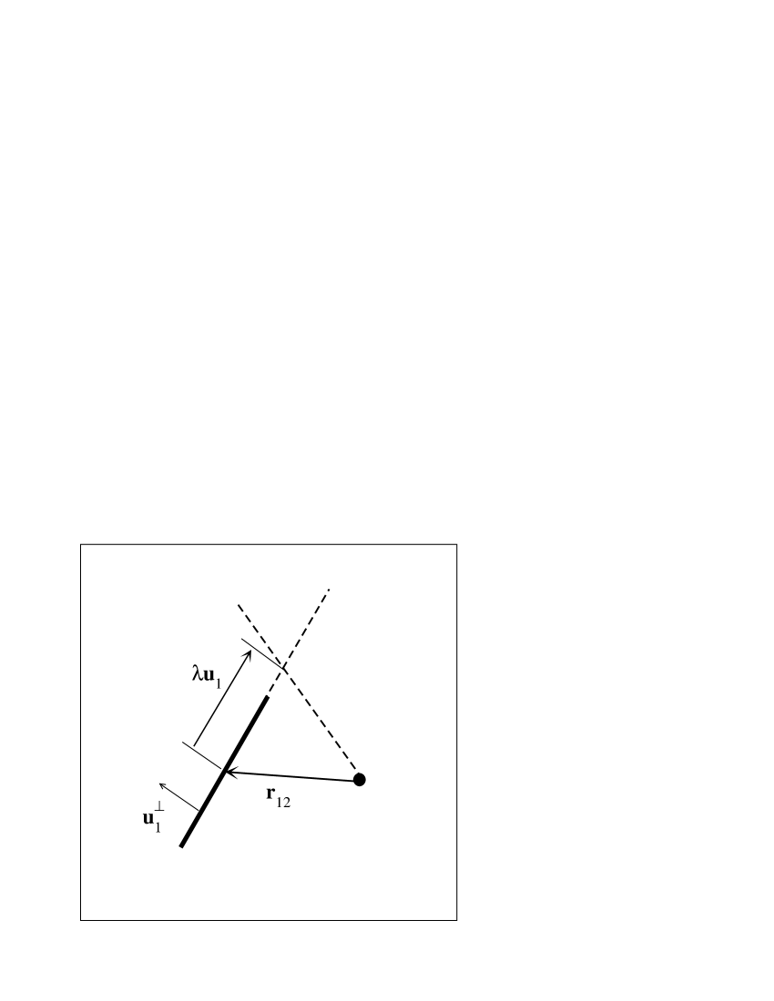
Figure 1: Geometry of the needle and a point in the plane: ${\bf r}_{12}$ denotes a vector joining the point labeled $2$ and the center of the needle; ${\bf u}_{1}$ is a unit vector along the axis of the needle, $\lambda$ is the algebraic distance between the center of the needle and the point of impact and ${\bf u}_{1}^{\perp}$ is a unit vector perpendicular to the axis of the needle. For a collision to occur one requires that $|\lambda|\leq L/2$ when the point lies on the line defined by the needle; i.e. when Eq.(1) is satisfied.

The pre- and post-collisional quantities (the latter are labeled with a prime) obey the usual conservation laws:

• Total momentum conservation

  $$M{\bf v^{\prime}}_{1}+m{\bf v^{\prime}}_{2}=M{\bf v}_{1}+m{\bf v}_{2}.$$ (3)

• Angular momentum conservation with respect to the point of contact

  $$I\omega^{\prime}_{1}{\bf k}=I\omega_{1}{\bf k}+M\lambda{\bf u}_{1}\land\left({\bf v^{\prime}}_{1}-{\bf v}_{1}\right),$$ (4)

  where ${\bf k}$ is a unit vector perpendicular to the plane such that ${\bf k}={\bf u}_{1}\land{\bf u}_{1}^{\perp}$.

As a result of the collision, the relative velocity of the contacting points changes instantaneously according to the following relations:

$${\bf V^{\prime}}.{\bf u}_{1}^{\perp} =-\alpha{\bf V}.{\bf u}_{1}^{\perp}$$ (5)

$${\bf V^{\prime}}.{\bf u}_{1} ={\bf V}_{.}{\bf u}_{1}$$ (6)

where $\alpha$ denotes the normal restitution coefficient. For the sake of simplicity we have taken the tangential restitution coefficient equal to one. This choice is reflected in the form of Eq. (6).

By combining Eqs. (2)- (5) one obtains, after some algebra, the change of the needle momentum $\Delta{\bf p}=M({\bf v}^{\prime}_{1}-{\bf v}_{1})$

$$\Delta{\bf p}.{\bf u}_{1}^{\perp}=-\frac{(1+\alpha){\bf V}.{\bf u}_{1}^{\perp}}{\frac{1}{m}+\frac{1}{M}+\frac{\lambda^{2}}{I}}.$$ (7)

The inelastic collision leads to a loss of translational kinetic energy,

$$\Delta E_{1}^{T} =\frac{M}{2}\left(({\bf v}^{\prime}_{1})^{2}-({\bf v}_{1})^{2}\right)$$

$$=\Delta{\bf p}.{\bf v}_{1}+\frac{1}{M}\frac{\Delta{\bf p}^{2}}{2}$$

$$=-(1+\alpha)\frac{{\bf V}.{\bf u}_{1}^{\perp}{\bf v}_{1}.{\bf u}_{1}^{\perp}.}{\frac{1}{m}+\frac{1}{M}+\frac{\lambda^{2}}{I}}+\frac{M}{2}\frac{(1+\alpha)^{2}({\bf V}.{\bf u}_{1}^{\perp})^{2}}{\left(\frac{1}{m}+\frac{1}{M}+\frac{\lambda^{2}}{I}\right)^{2}},$$ (8)

and rotational energy,

$$\Delta E_{1}^{R} =\frac{I}{2}\left((\omega^{\prime}_{1})^{2}-(\omega_{1})^{2}\right)$$

$$=-\frac{\lambda(1+\alpha)}{2}\frac{{\bf V}.{\bf u}_{1}^{\perp}(\omega_{1}^{\prime}+\omega_{1})}{\frac{1}{m}+\frac{1}{M}+\frac{\lambda^{2}}{I}}$$

$$=-\lambda(1+\alpha)\frac{{\bf V}.{\bf u}_{1}^{\perp}\omega_{1}}{\frac{1}{m}+\frac{1}{M}+\frac{\lambda^{2}}{I}}+\frac{\lambda^{2}(1+\alpha)^{2}({\bf V}.{\bf u}_{1}^{\perp})^{2}}{I\left(\frac{1}{m}+\frac{1}{M}+\frac{\lambda^{2}}{I}\right)^{2}}.$$ (9)

III Pseudo-Liouville equation

For particles with hard-core interactions, the kinetic evolution of $N$-particle distribution $f({\bf r}^{N},{\bf v}^{N})$ is described by a pseudo-Liouville operator, where ${\bf r}^{N}$ is a short-hand notation for the positions (and internal degrees of freedom, i.e. angle $\theta_{1}$ with the $x$-axis for the needle) of $N$ particles and ${\bf v}^{N}$ for their velocities (and angular velocities for the needle). Originally derived for spheres and elastic collisionsEDHV69 , the formalism has been extended to systems composed of inelastic particles. Since collisions are instantaneousVNE00 ; BMD96 , the pseudo-Liouville operator $L({\bf r}^{N},{\bf v}^{N})=L^{0}({\bf r}^{N})+\sum_{i<j}\overline{T}_{ij}$ is the sum of the free particle streaming operator $L^{0}({\bf r}^{N})$ and of the sum of two-body collision operators $\overline{T}_{ij}$. Since we are interested in the homogeneous state, the distribution function $f({\bf v}_{1},\omega_{1})$ of the needle system is described by

$$\frac{\partial f({\bf v}_{1},\omega_{1})}{\partial t}=N\int\frac{d\theta_{1}}{2\pi}\int d{\bf v_{2}}\int d{\bf r}_{2}\overline{T}_{12}f({\bf v}_{1},\omega_{1},{\bf v}_{2})$$ (10)

where $N$ is the total number of points, $f({\bf v}_{1},\omega_{1},{\bf v}_{2})$ the distribution function of the needle and a point, and $\overline{T}_{12}$ is the collision operator between a needle and a point.

The assumption of molecular chaos yields a factorization of the two body distribution $f({\bf v}_{1},\omega_{1},{\bf v}_{2})=f({\bf v}_{1},\omega_{1})\Phi({\bf v}_{2})$, where $\Phi({\bf v}_{2})$ denotes the point distribution function. Since the point particles are thermalized, a stationary state for the system (tracer needle and points) can be reached, and one finally obtains for the needle distribution

$$\int d\theta_{1}\int d{\bf v_{2}}\int d{\bf r}_{2}\overline{T}_{12}f({\bf v}_{1},{\bf\omega}_{1})\Phi({\bf v}_{2})=0$$ (11)

where

$$\Phi({\bf v}_{2})\propto\exp\left(-\frac{m{\bf v}_{2}^{2}}{2T}\right)$$ (12)

where $T$ is the temperature of the bath.

To build the point-needle collision operator, $\overline{T}_{12}$, one must include the change in quantities (i.e. velocity and angular momentum) produced during the infinitesimal time interval of the collision. This operator is different from zero only if the two particles are in contact and if the particles were approaching just before the collisionAHZ00 . The explicit form of the operator is

$$\overline{T}_{12} \propto\Theta(L/2-|\lambda|)\delta(|{\bf r}_{12}.{\bf u}_{1}^{\perp}|-0^{+})$$

$$\left|\frac{d|{\bf r}_{12}.{\bf u}_{1}^{\perp}|}{dt}\right|\Theta\left(-\left|\frac{d|{\bf r}_{12}.{\bf u}_{1}^{\perp}|}{dt}\right|\right)(b_{12}-1),$$ (13)

where $b_{12}$ is an operator that changes pre-collisional quantities to post-collisional quantities and $\Theta(x)$ is the Heaviside function.

The other terms of the collision operator correspond to the necessary conditions of contact $\Theta(L/2-|\lambda|)\delta(|{\bf r}_{12}.{\bf r}_{1}^{\perp}|-0^{+})$, and approach $\Theta\left(-\left|\frac{d|{\bf r}_{12}.{\bf u}_{1}^{\perp}|}{dt}\right|\right)$.

For an isotropic tracer particle in an isotropic particle bath, Martin and PiaseckiMP99 solved the stationary Enskog-Boltzmann equation, showing that the velocity distribution of the tracer particle remains gaussian in a thermalized bath. It is worth noting that for finite dilutions, the velocity distribution function is not MaxwellianBT02 , but the deviations from the gaussian shape of the distribution function of the velocities (that can be calculated in a perturbative way) yields small corrections to the estimate of the granular temperature. More significant deviations are expected for finite dilution systemsBMP02 .

For a mixture of a needle and points, one can show that a Maxwell distribution of the needle angular and translational momenta cannot be a solution of the stationary Enskog-Boltzmann equation even for the case of an infinitely diluted needle. This is due to the fact that the change of momentum depends on the location of the point of impact on the needle (the right-hand side of Eq. (7) depends on $\lambda$). However, we impose gaussian distributions for the translational and angular velocities of the needle. We show below that this is a very good approximation.

In the stationary state, the loss of translational and rotational kinetic energies is on average zero and can be expressed by means of the collision operator

$$\langle\Delta E_{1}^{T}\rangle =\langle\overline{T}_{12}f({\bf v}_{1},{\bf\omega}_{1})\Phi({\bf v}_{2})E_{1}^{T}({\bf v}_{1})\rangle=0$$

$$\langle\Delta E_{1}^{R}\rangle =\langle\overline{T}_{12}f({\bf v}_{1},{\bf\omega}_{1})\Phi({\bf v}_{2})E_{1}^{R}({\bf\omega}_{1})\rangle=0$$ (14)

where the brackets denote an average over the independent variables. This corresponds to taking the second moments of the distribution function of the needle. After substitution of the collision operator (Eq.(III)), one obtains explicitly for the translational kinetic energy

$$\int...\int d{\bf r}_{2}d{\bf v}_{1}d{\bf v}_{2}d\omega_{1}d\theta_{1}\Theta(L/2-|\lambda|)\delta(|{\bf r}_{12}.{\bf u}_{1}^{\perp}|-0^{+})$$

$$\left|\frac{d|{\bf r}_{12}.{\bf u}_{1}^{\perp}|}{dt}\right|\Theta\left(-\left|\frac{d|{\bf r}_{12}.{\bf u}_{1}^{\perp}|}{dt}\right|\right)f({\bf v}_{1},{\bf\omega}_{1})\Phi({\bf v}_{2})\Delta E^{T}_{1}=0.$$ (15)

A similar equation can be written for rotational kinetic energy. The needle distribution function $f({\bf v}_{1},\omega_{1})$ is then given by

$$f({\bf v}_{1},\omega_{1})\propto\exp\left(-\frac{M{\bf v_{1}}^{2}}{2\gamma_{T}T}-\frac{I{\bf\omega_{1}}^{2}}{2\gamma_{R}T}\right),$$ (16)

where $\gamma_{T}$ and $\gamma_{R}$ are the ratios of the translational and rotational needle temperatures to the bath temperature, respectively.

By inserting Eq. (16) in Eq. (III) and in the corresponding equation for the rotational energy one obtains, after some tedious but straightforward calculation (outlined in Appendix A), the following set of equations

$$\int_{0}^{1}dxb\frac{\sqrt{1+akx^{2}}}{1+kx^{2}} =\frac{1+\alpha}{2}\int_{0}^{1}dx\frac{(1+akx^{2})^{3/2}}{(1+kx^{2})^{2}},$$ (17)

$$\int_{0}^{1}dxax^{2}\frac{\sqrt{1+akx^{2}}}{1+kx^{2}} =\frac{1+\alpha}{2}\int_{0}^{1}dx\frac{x^{2}(1+akx^{2})^{3/2}}{(1+kx^{2})^{2}},$$ (18)

where

$$k=\frac{L^{2}}{4I\left(\frac{1}{m}+\frac{1}{M}\right)},$$ (19)

$$a=\gamma_{R}\frac{(M+m)}{M+m\gamma_{T}},$$ (20)

and

$$b=\gamma_{T}\frac{M+m}{M+m\gamma_{T}}.$$ (21)

Explicit expressions for the integrals appearing in Eqs. (17) and (18) are given in Appendix B. Eq. (18) is an implicit equation for $a$ that, for a given value of $\alpha$, can be solved with standard numerical methods. $b$ is then easily obtained by calculating the ratio of integrals of Eq. (17). Finally, from the values of $a$ and $b$, $\gamma_{T}$ and $\gamma_{R}$ can be obtained from Eqs.(20)-(21).

IV Results

We first note that for the elastic case, $\alpha=1$, we have the solution $a=b=1$ which gives $\gamma_{T}=1$ and since $a/b=\gamma_{R}/\gamma_{T}$, $\gamma_{R}=1$ which corresponds to the equilibrium caseFD81 ; FD83 .

Figure 2 shows the ratio of the translational temperature to the bath temperature and of the rotational temperature to the bath temperature for a homogeneous needle ($I=ML^{2}/12$) whose mass is equal to the mass of a bath particle. As the normal restitution coefficient decreases from $1$ to $0$ both ratios decrease monotonically from $1$ to a strictly positive value, such that the translational temperature is always larger the rotational temperature. An analogous situation has been noted for the free cooling of needles in three dimensionsAHZ00 .

Figure 3 shows the same ratios for an inhomogeneous needle ($I=ML^{2}/16$) corresponding to relatively lighter ends and a heavier center. Again the translational temperature is always larger than the rotational temperature, and the differences are greater than for a homogeneous needle. The difference between the two temperatures vanishes in the limit of very large moment of inertia. Contrary to the free cooling state of needles AHZ00 , there is no “critical” value of the moment of inertia above which the rotational temperature is larger than the translational temperature.

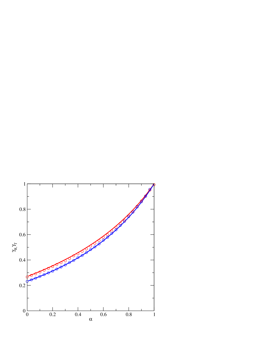
Figure 2: Ratio of the translational (full curve) $\gamma_{T}$ and rotational $\gamma_{R}$ (dashed curve) granular temperature to the temperature of the bath versus the normal restitution coefficient $\alpha$ for a homogeneous needle with $M=m$.

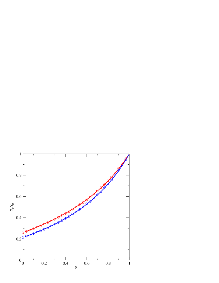
Figure 3: Ratio of the translational (full curve) $\gamma_{T}$ and rotational $\gamma_{R}$ (dashed curve) granular temperature to the temperature of the bath versus the normal restitution coefficient $\alpha$ for an inhomogeneous needle ($I=ML^{2}/16$)with $M=m$.

We now return to consideration of a homogeneous needle and investigate the effect of varying the mass ratio, $m/M$, at constant normal restitution coefficient. When $m/M\to 0$, $k\to 0$, which gives $a=b=(1+\alpha)/2$. Hence, for very light bath particles, equipartition between translational and rotational granular temperatures is asymptotically obtained and we have

$$\gamma_{R}=\gamma_{T}=\frac{1+\alpha}{2}.$$ (22)

This same limit is obtained for a spherical tracer particle MP99 . We conjecture that the result is independent of the shape of the tracer particle and the dimension.

Figure 4 displays the variation with the mass ratio of the translational and rotational temperature of the tracer needle. Note that when the mass of the bath particles is very small compared to the needle particle, the two curves go to the limit given by Eq. (22).

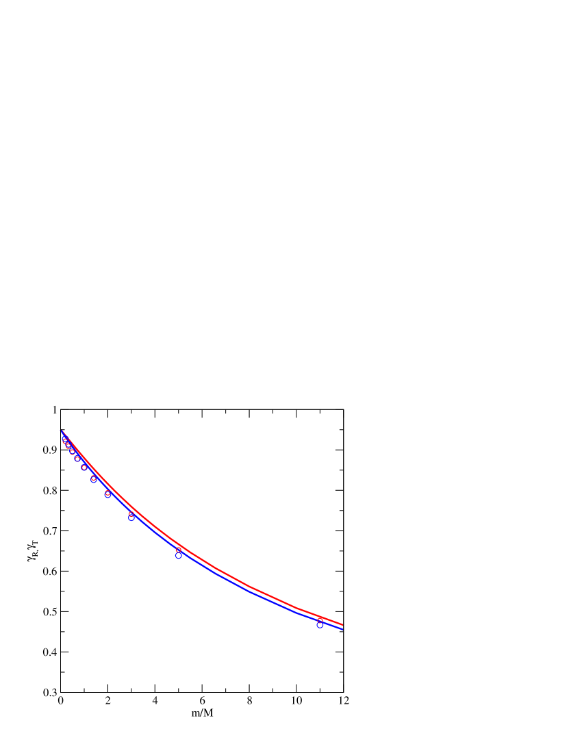
Figure 4: Ratio of the translational (full curve) $\gamma_{T}$ and rotational $\gamma_{R}$ (dashed curve) granular temperature to the temperature of the bath versus the ratio of the masses $m/M$ for a homogeneous needle ($I=ML^{2}/12$) and $\alpha=0.9$.

V Simulation

In order to assess the accuracy of the theory we developed a Direct Simulation Monte Carlo (DSMC) code to obtain numerical solutions of the non-linear homogeneous Boltzmann equation. The simulation generates a sequence of collisions with a variable time interval between each.

At the beginning of each step, we first calculate the total flux of colliding particles on both sides of the needle which is a function of the component of the velocity of the center of mass normal to the length of the needle ${\bf v}_{1}.{\bf u}_{1}^{\perp}$ and the angular velocity $\omega$. Next a waiting time to the next collision is sampled from an exponential distribution with rate constant equal to the total flux. The needle is rotated at its current angular velocity to the point of collision. The location of the collision is then selected with a probability proportional to the position dependent flux. The ratio of the flux on the left hand side to the total flux is then compared to a uniform random number between zero and one. If the ratio is greater than the random number, the collision occurs on the right; otherwise is occurs on the left. The normal component of the colliding point is then selected from a gaussian flux. Finally, the collision rules are applied and the normal velocity and angular velocity of the needle are updated.

The simulation results for $10^{7}$ collisions per run are compared with the theory in Figs. 2- 3. Although the theory is not exact, the agreement is excellent. The discrepancy between simulation and theory is never greater than $1\%$ whatever the value of the restitution coefficient. In Fig. 4, when the mass of the needle increases, the granular temperatures obtained by simulation are slightly smaller than the analytical result.

Fig. 5 and Fig. 6 show the translational and angular velocity distributions, respectively, for two different values of the normal restitution coefficient ($0.5$ and $0.9$). On the scale of the plot, the simulated distributions are in quantitative agreement with gaussian distributions at the corresponding theoretical granular temperature, confirming the validity of employing the latter in the theory.

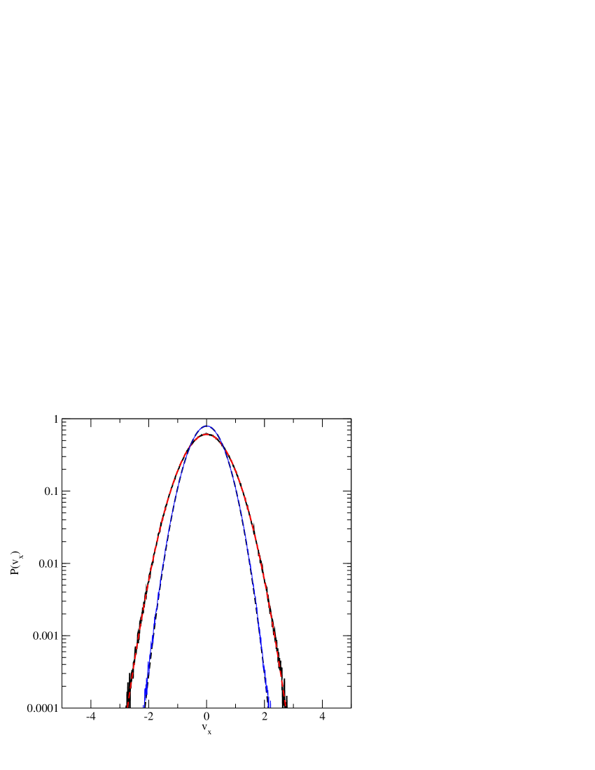
Figure 5: Distribution of the normal velocity component of the needle for two values of the normal restitution coefficient, $\alpha=0.5$ and $\alpha=0.9$ (broader curve). The solid (noisy) curves are the simulation results and the dashed curves correspond to Gaussian distributions of velocity evaluated for the corresponding theoretical granular temperature.

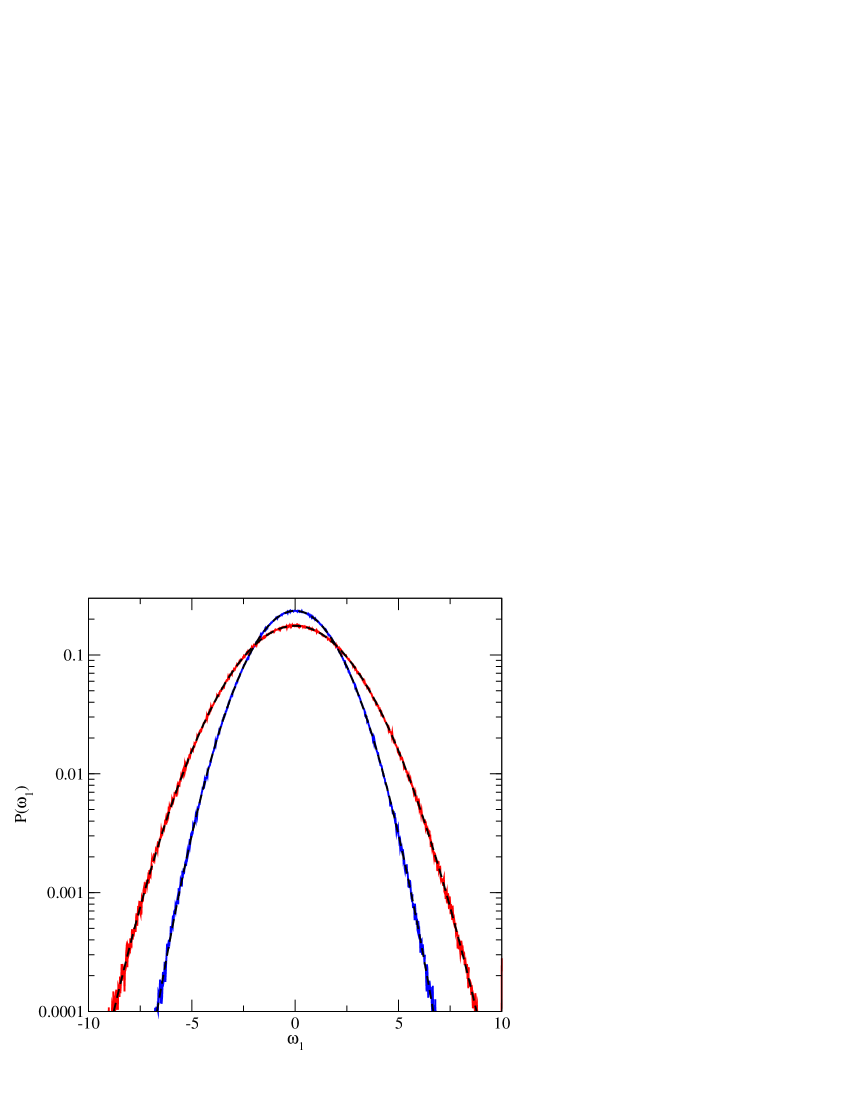
Figure 6: Same as 5, except the angular velocity is shown.

VI Conclusion

We have shown that the translational and rotational granular temperatures of an anisotropic tracer particle immersed in a bath of point particles depend on the ratio of the masses of a point and the needle and the moment of inertia. They are, in general, not equal and differ from the bath temperature. In addition, we found that equipartition is obtained asymptotically, regardless of the normal restitution coefficient, for very light bath particles. We expect this to be a general feature, i.e. in higher dimensions and for arbitrary shaped anisotropic particles. It should be possible to test this prediction experimentally.

Appendix A Needle average energy loss

As for binary mixtures of spheresBT02 , we use a gaussian ansatz for the distribution functions and introduce two different temperatures corresponding to the translational and rotational degrees of freedom of the needle. The homogeneous distribution functions of the needle and of the points are then given respectively by

$$f({\bf v}_{1},\omega_{1})\sim\exp\left(-\frac{M{\bf v}_{1}^{2}\gamma_{T}^{-1}}{2T}-\frac{I\omega_{1}^{2}\gamma_{R}^{-1}}{2T}\right),$$ (23)

$$\Phi({\bf v}_{2})\sim\exp\left(-\frac{m{\bf v}_{2}^{2}}{2T}\right),$$ (24)

where $T$ is the temperature of the bath, $\gamma_{T}$ and $\gamma_{R}$ the ratio of the translational (and rotational) temperature of the needle to the bath temperature.

We introduce the vectors ${\boldsymbol{\chi}}$ and ${\boldsymbol{\nu}}$ such that

$${\boldsymbol{\chi}} =\frac{1}{\sqrt{2T(M\gamma_{T}+m)}}\left(M{\bf v}_{1}+m{\bf v}_{2}\right)$$ (25)

$${\boldsymbol{\nu}} =\sqrt{\frac{mM}{2T(M\gamma_{T}+m)\gamma_{T}}}\left({\bf v}_{1}+\gamma_{T}{\bf v}_{2}\right)$$ (26)

The scalar product ${\bf V}.{\bf u}_{1}^{\perp}$ can be expressed as

$${\bf V}.{\bf u}_{1}^{\perp} =\sqrt{\frac{2T}{mM\gamma_{T}}}\left[\left(\gamma_{T}-1\right){\boldsymbol{\chi}}.{\bf u}_{1}^{\perp}\right.$$

$$\left.+\sqrt{\gamma_{T}}\left(\sqrt{\frac{m}{M}}+\sqrt{\frac{M}{m}}\right){\boldsymbol{\nu}}.{\bf u}_{1}^{\perp}\right]$$ (27)

Let us introduce $\xi=\omega_{1}\sqrt{\frac{I}{2T\gamma_{R}}}$. The translational energy loss is given by the formula

$$\sum_{p=\pm 1}\int d\lambda\int d\theta_{1}\int d{\boldsymbol{\chi}}\int d{\boldsymbol{\nu}}\int d\omega_{1}$$

$$\exp\left(-{\boldsymbol{\chi}}^{2}-{\boldsymbol{\nu}}^{2}-\xi^{2}\right)|{\bf V}.{\bf u}_{1}^{\perp}|\Theta(p{\bf V}.{\bf u}_{1}^{\perp})\Theta\left(|\lambda|-\frac{L}{2}\right)\Delta E_{1}^{T}.$$ (28)

Since Eq. (A) depends only on ${\boldsymbol{\chi}}.{\bf u}_{1}^{\perp}$ and ${\boldsymbol{\nu}}.{\bf u}_{1}^{\perp}$ , one can freely integrate over the direction of ${\bf u}_{1}$ for the vectors ${\boldsymbol{\chi}}$ and ${\boldsymbol{\nu}}$. The integration over $\theta_{1}$ can be easily performed. If we introduce the three dimensional vectors ${\bf G}$ and ${\bf s}$ with components:

$${\bf G}= \left(G_{1},G_{2},G_{3}\right)$$

$$= \left(\sqrt{\frac{2T}{M\gamma_{T}+m}}(\gamma_{T}-1),\sqrt{\frac{2T\gamma_{T}}{M\gamma_{T}+m}}\frac{m+M}{\sqrt{mM}},\right.$$

$$\left.\lambda\sqrt{\frac{2T\gamma_{R}}{I}}\right)$$ (29)

and

$${\bf s}= \left(s_{1},s_{2},s_{3}\right)$$

$$\left({\boldsymbol{\chi}}.{\bf u}_{1}^{\perp},{\boldsymbol{\nu}}.{\bf u}_{1}^{\perp},\xi\right)$$ (30)

By inserting Eq. (II) in Eq. (A), the average energy loss can be rewritten as

$$\sum_{p=\pm 1}\int d\lambda\int d{\bf s}\exp\left(-{\bf s}^{2}\right)|{\bf G}.{\bf s}|\Theta(p{\bf G}.{\bf s})\Theta\left(|\lambda|-\frac{L}{2}\right)$$

$$\left[-\frac{(1+\alpha){\bf G}.{\bf s}}{\frac{1}{m}+\frac{1}{M}+\frac{\lambda^{2}}{I}}\sqrt{\frac{2T}{M\gamma_{T}+m}}\left(\gamma_{T}s_{1}+\sqrt{\frac{m\gamma_{T}}{M}}s_{2}\right)\right.$$

$$\left.+\frac{(1+\alpha)^{2}({\bf G}.{\bf s})^{2}}{2M\left(\frac{1}{m}+\frac{1}{M}+\frac{\lambda^{2}}{I}\right)^{2}}\right]$$ (31)

By defining a new coordinate system in which the $z$-axis is parallel to ${\bf G}$, one find that the integrals of Eq. (A) involve gaussian integrals of the form

$$\int d{\bf s}\exp\left(-{\bf s}^{2}\right)(|{\bf G}|s_{z})^{2}\Theta(\pm s_{z})G_{i}s_{z}=\frac{\pi}{8}|{\bf G}|^{2}G_{i}$$ (32)

and

$$\int d{\bf s}\exp\left(-{\bf s}^{2}\right)(|{\bf G}|s_{z})^{3}\Theta(\pm s_{z})=\frac{\pi}{8}|{\bf G^{3}}|$$ (33)

which finally leads to Eq. (17). The equation for rotational energy is derived following exactly the same procedure.

Appendix B Integrals

The integrals appearing in Eqs. (17) and (18) can be evaluated explicitly. For completeness, we give below their analytical expressions

$$I_{1} =\int_{0}^{1}dx\frac{\sqrt{1+akx^{2}}}{1+kx^{2}}$$

$$=\sqrt{\frac{a}{k}}\ln(\sqrt{ak}+\sqrt{1+ak})$$

$$+\sqrt{\frac{1-a}{k}}\arctan\left(\sqrt{\frac{(1-a)k}{1+ak}}\right)$$ (34)

The integral $I_{2}$ is defined as

$$I_{2}=\int_{0}^{1}dx\frac{(1+akx^{2})^{3/2}}{(1+kx^{2})^{2}}$$ (35)

and satisfies the equation

$$I_{2}=I_{1}-(a-1)k\left.\frac{\partial\int_{0}^{1}dx\frac{\sqrt{1+akx^{2}}}{1+dx^{2}}}{\partial d}\right|_{d=k}$$ (36)

which gives

$$I_{2} =\frac{a^{3/2}}{\sqrt{k}}\ln(\sqrt{ak}+\sqrt{1+ak})+\frac{(1-a)\sqrt{1+ak}}{2(1+k)}$$

$$\frac{1+a-2a^{2}}{2\sqrt{k(1-a)}}\arctan\left(\sqrt{\frac{(1-a)k}{1+ak}}\right)$$ (37)

$$I_{3} =\int_{0}^{1}dx\frac{x^{2}\sqrt{1+akx^{2}}}{1+kx^{2}}$$

$$=\frac{1}{k}\left(\int_{0}^{1}dx\sqrt{1+akx^{2}}-I_{1}\right)$$ (38)

$$=\frac{\sqrt{ak+1}}{2k}\frac{1-2a}{\sqrt{a}k^{3/2}}+\ln(\sqrt{ak}+\sqrt{1+ak})$$

$$-\frac{\sqrt{1-a}}{k^{3/2}}\arctan\left(\sqrt{\frac{(1-a)k}{1+ak}}\right)$$ (39)

Finally, one has

$$I_{4}=\int_{0}^{1}dx\frac{x^{2}(1+akx^{2})^{3/2}}{(1+kx^{2})^{2}}$$ (40)

which satisfy the algebraic equation

$$I_{2}+kI_{4} =aJ_{1}+(a-1)I_{1}$$ (41)

which gives

$$I_{4} =\frac{\sqrt{1+ak}(ak-1+2a)}{2k(k+1)}$$

$$+\frac{\sqrt{a}(3-4a)}{2k^{3/2}}\ln(\sqrt{ak}+\sqrt{1+ak})$$

$$+\frac{\sqrt{1-a}(1-4a)}{2k^{3/2}}\arctan\left(\sqrt{\frac{(1-a)k}{1+ak}}\right)$$ (42)

References

• (1) R. D. Wildman and D. J. Parker, Phys. Rev. Lett. 88, 064301 (2002).
• (2) K. Feitosa and N. Menon, Phys. Rev. Lett. 88, 198301 (2002).
• (3) A. Barrat and E. Trizac, Granul. Matter 4, 57 (2002).
• (4) A. Barrat and E. Trizac, Phys. Rev. E 66, 051303 (2002).
• (5) P. E. Krouskop and J. Talbot, cond-mat/0303263.
• (6) P. A. Martin and J. Piasecki, Europhys. Lett 46, 613 (1999).
• (7) T. Aspelmeier, T. M. Huthmann, and A. Zippelius, in Granular Gases, edited by S. Luding and T. Poschel (Springer, Berlin, 2000), Chap. Free cooling of particles with rotational degrees of freedom, p. 31.
• (8) M. Huthmann, T. Aspelmeier, and A. Zippelius, Phys. Rev. E 60, 654 (1999).
• (9) M. H. Ernst, J. R. Dorfman, W. R. Hoegy, and J. M. J. van Leeuwen, Physica 45, 127 (1969).
• (10) T. van Noije and M. Ernst, in Granular Gases, edited by S. Luding and T. Poschel (Springer, Berlin, 2001), Chap. Kinetic Theory of Granular Gases, p. 3.
• (11) J.J. Brey, F. Moreno, and J.W. Dufty, Phys. Rev. E 54, 445 (1996).
• (12) T. Biben, P. A. Martin, and J. Piaseski, Physica A 310, 308 (2002).
• (13) D. Frenkel and J.F. Maguire, Phys. Rev. Lett. 47, 1025 (1981).
• (14) D. Frenkel and J. Maguire, Mol. Phys. 49, 503 (1981).