Ornstein-Zernike equation and Percus-Yevick theory for molecular crystals

Abstract

We derive the Ornstein-Zernike equation for molecular crystals of axially symmetric particles and apply the Percus-Yevick approximation to this system. The one-particle orientational distribution function $\rho^{(1)}(\Omega)$ has a nontrivial dependence on the orientation $\Omega$, in contrast to a liquid, and is needed as an input. Despite some differences, the Ornstein-Zernike equation for molecular crystals has a similar structure as for liquids. We solve both equations numerically for hard ellipsoids of revolution on a simple cubic lattice. Compared to molecular liquids, the orientational correlators in direct and reciprocal space exhibit less structure. However, depending on the lengths $a$ and $b$ of the rotation axis and the perpendicular axes of the ellipsoids, respectively, different behavior is found. For oblate and prolate ellipsoids with $b\gtrsim 0.35$ (in units of the lattice constant), damped oscillations in distinct directions of direct space occur for some of the orientational correlators. They manifest themselves in some of the correlators in reciprocal space as a maximum at the Brillouin zone edge, accompanied by a maximum at the zone center for other correlators. The oscillations indicate alternating orientational fluctuations, while the maxima at the zone center originate from nematic-like orientational fluctuations. For $a\lesssim 2.5$ and $b\lesssim 0.35$, the oscillations are weaker, leading to no marked maxima at the Brillouin zone edge. For $a\gtrsim 3.0$ and $b\lesssim 0.35$, no oscillations occur any longer. For many of the orientational correlators in reciprocal space, an increase of $a$ at fixed $b$ or vice versa leads to a divergence at the zone center ${\bf q}={\bf 0}$, consistent with the formation of nematic-like long range fluctuations, and for some oblate and prolate systems with $b\lesssim 1.0$ a simultaneous tendency to divergence of few other correlators at the zone edge is observed. Comparison of the orientational correlators with those from MC simulations shows satisfactory agreement. From these simulations we also obtain a phase boundary in the $a-b$-plane for order-disorder transitions.

I Introduction

The experimental, numerical and analytical study of structural properties of simple liquids is a well established discipline of condensed matter physics. In the center of such investigations is the static structure factor $S(q)$. There are powerful integral equations allowing an approximate calculation of $S(q)$ J.-P. Hansen, I. R. McDonald (1990). The starting point is the Ornstein-Zernike (OZ) equation, relating the total correlation function $h(q)$ and the direct correlation function $c(q)$. An additional closure relation, like the Percus-Yevick (PY) approximation, then allows to determine $h(q)$, from which $S(q)$ follows from

$$S(q)=1+\rho h(q),$$ (1)

where $\rho$ is the number density of the liquid. Application of the PY approximation to a liquid of hard spheres yields good agreement with the exact result for intermediate values of $\rho$ J.-P. Hansen, I. R. McDonald (1990). However, the crystallization of hard spheres cannot be described by PY theory.

The extension of the OZ equation and the PY approximation (or other closure relations) to molecular liquids is straightforward J.-P. Hansen, I. R. McDonald (1990); C. G. Gray, K. E. Gubbins (1984) and has been applied extensively (see, e.g., J. Ram, R. C. Singh, Y. Singh (1994); M. Letz, A. Latz (1999)). As for simple liquids, PY theory usually does not yield an order-disorder phase transition. Therefore, it was quite surprising that a recent application of the molecular version of that theory to a liquid of hard ellipsoids of revolution with aspect ratio $X_{0}$ has allowed the location of a phase boundary in the $\rho-X_{0}$-plane, at which a transition to a nematic phase takes place M. Letz, A. Latz (1999).

Much less analytical work exists for molecular crystals J. D. Wright (2001); J. N. Sherwood (1979). These are crystalline materials with, e.g., a molecule at each lattice site. One of the main interests concerns phase transitions of the translational and rotational degrees of freedom (see, e.g., the review M. H. Müser (1998)). These transitions are influenced by the translation-rotation coupling R. M. Lynden-Bell, K. H. Michel (1994). But one also expects phase transitions if the crystal is assumed to be rigid. For instance, let us fix hard ellipsoids of revolution with their centers at the lattice sites of, e.g., a simple cubic lattice with lattice constant equal to one. With $a$ and $b$ the lengths of the rotation axis and the perpendicular axes of the ellipsoids, respectively, an increase of $a$ for fixed $b$ may yield at a critical length $a_{c}(b)$ a transition to an orientationally ordered phase, because the entropy of the ordered phase is larger than that of the disordered phase.

Besides phase transitions, the study of the orientational structure of molecules on a rigid lattice is of interest, too. Changing temperature will influence the steric hindrance between the molecules. The same happens for hard ellipsoids when changing $a$ and $b$. Analogous to simple and molecular liquids, one can quantify such static orientational properties by the one-particle orientational distribution $\rho^{(1)}(\Omega)$ J. N. Sherwood (1979); M. Yvinec, R. Pick (1980); R. M. Lynden-Bell, K. H. Michel (1994); W. Breymann, R. Pick (1988, 1989, 1994) and by the orientational correlation function $G_{nn^{\prime}}(\Omega,\Omega^{\prime})$, where the orientation $\Omega$ can be characterized, e.g., by the Euler angles $(\phi,\theta,\chi)$ or, for axially symmetric particles, by $(\phi,\theta)$. Then the following questions arise: How to compute $\rho^{(1)}(\Omega)$ and, above all, the correlation function $G_{nn^{\prime}}(\Omega,\Omega^{\prime})$ by an analytical method? Does the result for $G_{nn^{\prime}}(\Omega,\Omega^{\prime})$ allow to locate a phase boundary where a transition to an orientationally ordered phase occurs? To provide answers to these questions is the main motivation of our contribution.

Our paper is organized as follows. In Sec. II we will introduce the model and the basic physical quantities like the one-particle distribution function $\rho^{(1)}(\Omega)$ and the orientational correlation function $G_{nn^{\prime}}(\Omega,\Omega^{\prime})$. The analytical approach of calculating $G_{nn^{\prime}}(\Omega,\Omega^{\prime})$ or its transform $S_{\lambda\lambda^{\prime}}({\bf q})$ from the OZ equation in combination with the PY approximation is described in Sec. III. Results from PY theory for hard ellipsoids of revolution on a simple cubic lattice will be shown in Sec. IV and compared with those from MC simulations. This section also presents a short discussion of the phase transition for the ellipsoids from an orientationally disordered to an ordered phase. The final Sec. V contains a discussion of the results and some conclusions. We add a couple of appendices, including extensive technical manipulations needed in Secs. III, IV.

II Distribution and correlation functions and their symmetries

II.1 One- and two-particle distribution and correlation functions

We consider a three-dimensional periodic lattice with $N$ lattice sites and periodic boundary conditions. If the $n$-th lattice site has the position ${\bf x}_{n}$, the difference between two sites is the vector ${\bf x}_{nn^{\prime}}={\bf x}_{n^{\prime}}-{\bf x}_{n}$. We assume the lattice to be rigid with lattice constant equal to one. At each lattice site we fix a rigid molecule, not necessarily with its center of mass. Restricting to linear molecules, the orientation of the molecule at site $n$ is given by $\Omega_{n}=(\phi_{n},\theta_{n})\in S^{2}$. The third Euler angle $\chi_{n}$ is irrelevant for our purposes. Extension of our theoretical approach below to arbitrary molecules is straightforward. The interaction energy $V(\{\Omega_{n}\})$ is assumed to be pairwise and the classical Hamiltonian is given by

$$H(\{\Omega_{n}\},\{{\bf l}_{n}\})=\sum\limits_{n=1}^{N}\frac{1}{2}{\bf l}_{n}^{T}{\bf I}^{-1}(\Omega_{n}){\bf l}_{n}+V(\{\Omega_{n}\})\,,$$ (2)

where ${\bf l}_{n}$ and ${\bf I}(\Omega_{n})$, respectively, are the angular momentum and the tensor of inertia of the molecule at site $n$ in the space fixed frame. Since we will investigate static quantities only, the kinetic part of $H(\{\Omega_{n}\},\{{\bf l}_{n}\})$ does not matter.

In order to describe the orientational degrees of freedom, we introduce the microscopic one particle density $\rho_{n}(\Omega)$, $\Omega\in S^{2}$, at lattice site $n$ and its associated fluctuation defined by

$$\rho_{n}(\Omega) =\delta(\Omega|\Omega_{n})\,,$$ (3a)

$$\delta\rho_{n}(\Omega) =\rho_{n}(\Omega)-\langle\rho_{n}(\Omega)\rangle\,,$$ (3b)

where $\delta(\Omega|\Omega^{\prime})=\sin\theta\,\delta(\theta-\theta^{\prime})\delta(\phi-\phi^{\prime})$, and $\langle(\cdot)\rangle$ denotes canonical averaging with respect to $H(\{\Omega_{n}\},\{{\bf l}_{n}\})$. Note that the $\Omega_{n}$-dependence of $\rho_{n}$ and $\delta\rho_{n}$ is suppressed. The one-particle orientational distribution function is given by

$$\rho^{(1)}(\Omega)=\langle\rho_{n}(\Omega)\rangle\,,$$ (4)

which is $n$-independent due to the lattice translational invariance of $H(\{\Omega_{n}\},\{{\bf l}_{n}\})$, and the two-particle distribution is defined as

$$\rho^{(2)}_{nn^{\prime}}(\Omega,\Omega^{\prime})\equiv\rho^{(2)}_{{\bf x}_{nn^{\prime}}}(\Omega,\Omega^{\prime})=\langle\rho_{n}(\Omega)\rho_{n^{\prime}}(\Omega^{\prime})\rangle\,,\quad n\neq n^{\prime}\,.$$ (5)

Note that $\rho^{(2)}_{nn^{\prime}}$ is defined for $n\neq n^{\prime}$, only, and that the index pair $nn^{\prime}$ is fully equivalent to the vector ${\bf x}_{nn^{\prime}}$. Making use of Eqs. (3), it follows

$$\int\limits_{S^{2}}\rho^{(1)}(\Omega)\,d\Omega=1\,,$$ (6)

$$\int\limits_{S^{2}}\rho^{(2)}_{nn^{\prime}}(\Omega,\Omega^{\prime})\,d\Omega =\rho^{(1)}(\Omega^{\prime}) \quad(n\neq n^{\prime})\,,$$ (7a)

$$\int\limits_{S^{2}}\rho^{(2)}_{nn^{\prime}}(\Omega,\Omega^{\prime})\,d\Omega^{\prime} =\rho^{(1)}(\Omega) \quad(n\neq n^{\prime})\,.$$ (7b)

It is important to realize that in contrast to isotropic molecular liquids the one-particle distribution $\rho^{(1)}(\Omega)$ depends on $\Omega$. An additional important feature may occur for particles with hard core interaction, e.g. hard ellipsoids, which are big enough. In that case there may exist a non-empty subset $\bar{K}$ of $S^{2}$ such that $\rho^{(1)}(\Omega)=0$ for all $\Omega\in\bar{K}$. Hence, the orientation of each particle is restricted to the complement $K=S^{2}\setminus\bar{K}\subset S^{2}$. In the following, we need to distinguish between the two cases $K=S^{2}$ and $K\subset S^{2}$, where $K$ is the area on $S^{2}$ which can be reached by particle orientations. Clearly, it is $\rho^{(2)}_{nn^{\prime}}(\Omega,\Omega^{\prime})=0$, if $\rho^{(1)}(\Omega)=0$ or $\rho^{(1)}(\Omega^{\prime})=0$, but not vice versa. Three examples for $\rho^{(1)}(\Omega)$ are shown in Fig. 1, obtained from MC simulations for hard ellipsoids on a simple cubic lattice.

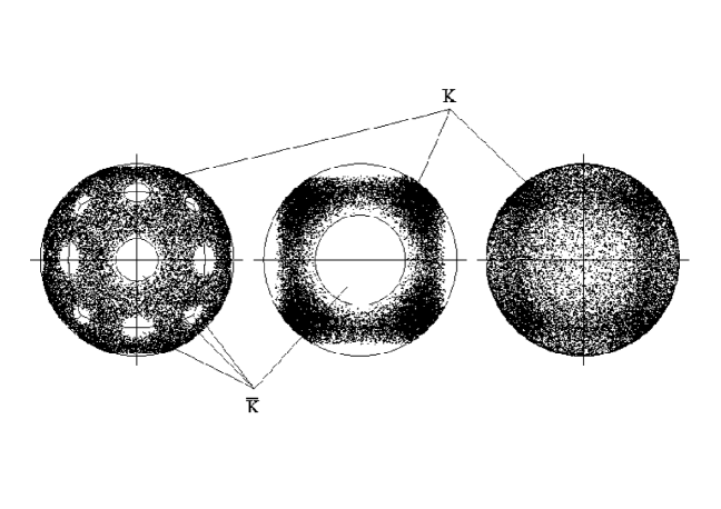
Figure 1: MC results for $\rho^{(1)}(\Omega)$ for hard ellipsoids of revolution with $a=3.6$, $b=0.24$ (left), $a=1.2$, $b=0.88$ (middle) and $a=0.56$, $b=1.1$ (right) on a sc lattice. Orientations on $S^{2}$ obtained from MC runs are projected along the fourfold lattice direction. Parts of $\bar{K}$ occur along the two-, three- and fourfold lattice directions, depending approximately on whether $\frac{a+b}{2}$ exceeds the site-site spacing along one of these directions. Some circles approximating the edges of the parts of $\bar{K}$ are shown as an aid for the eye.

Next, we introduce the orientational density-density correlation function $G_{nn^{\prime}}(\Omega,\Omega^{\prime})$. It is the correlation of the fluctuations of $\rho_{n}(\Omega)$ at lattice sites $n$ and $n^{\prime}$:

$$G_{nn^{\prime}}(\Omega,\Omega^{\prime})=\langle\delta\rho_{n}(\Omega)\delta\rho_{n^{\prime}}(\Omega^{\prime})\rangle\,.$$ (8)

By use of Eqs. (3)-(5) we get

$$G_{nn^{\prime}}(\Omega,\Omega^{\prime})= \;\delta_{nn^{\prime}}\rho^{(1)}(\Omega)\,\delta(\Omega|\Omega^{\prime})-\rho^{(1)}(\Omega)\rho^{(1)}(\Omega^{\prime})$$

$$+(1-\delta_{nn^{\prime}})\rho^{(2)}_{nn^{\prime}}(\Omega,\Omega^{\prime})\,.$$ (9)

$G_{nn^{\prime}}(\Omega,\Omega^{\prime})=G^{(s)}_{nn^{\prime}}(\Omega,\Omega^{\prime})+G^{(d)}_{nn^{\prime}}(\Omega,\Omega^{\prime})$ consists of a self part and a distinct part, which are explicitely

$$G^{(s)}_{nn^{\prime}}(\Omega,\Omega^{\prime}) =\delta_{nn^{\prime}}\left(\rho^{(1)}(\Omega)\delta(\Omega|\Omega^{\prime})-\rho^{(1)}(\Omega)\rho^{(1)}(\Omega^{\prime})\right)\,,$$ (10a)

$$G^{(d)}_{nn^{\prime}}(\Omega,\Omega^{\prime}) =\left(1-\delta_{nn^{\prime}}\right)\left(\rho^{(2)}_{nn^{\prime}}(\Omega,\Omega^{\prime})-\rho^{(1)}(\Omega)\rho^{(1)}(\Omega^{\prime})\right)\,.$$ (10b)

Due to the properties (6) and (7) of the particle distribution functions, $G_{nn^{\prime}}(\Omega,\Omega^{\prime})$ fulfills for all $nn^{\prime}$

$$\int\limits_{S^{2}}G_{nn^{\prime}}(\Omega,\Omega^{\prime})\,d\Omega=\int\limits_{S^{2}}G_{nn^{\prime}}(\Omega,\Omega^{\prime})\,d\Omega^{\prime}=0\,.$$ (11)

For the lattice system, the pair and total correlation functions $g_{nn^{\prime}}(\Omega,\Omega^{\prime})$ and $h_{nn^{\prime}}(\Omega,\Omega^{\prime})$ are introduced in the same manner as for a liquid J.-P. Hansen, I. R. McDonald (1990); C. G. Gray, K. E. Gubbins (1984):

$$g_{nn^{\prime}}(\Omega,\Omega^{\prime}) =\frac{\rho^{(2)}_{nn^{\prime}}(\Omega,\Omega^{\prime})}{\rho^{(1)}(\Omega)\,\rho^{(1)}(\Omega^{\prime})} \quad(n\neq n^{\prime})\,,$$ (12)

$$h_{nn^{\prime}}(\Omega,\Omega^{\prime}) =g_{nn^{\prime}}(\Omega,\Omega^{\prime})-1 \quad(n\neq n^{\prime})\,.$$ (13)

Here, some comments are in order. First, $g_{nn^{\prime}}$ and $h_{nn^{\prime}}$ are defined for $n\neq n^{\prime}$ only, and if $K\subset S^{2}$, for $\Omega,\Omega^{\prime}\in K$ only. Second, $h_{nn^{\prime}}(\Omega,\Omega^{\prime})$ in general obeys

$$\int\limits_{S^{2}}h_{nn^{\prime}}(\Omega,\Omega^{\prime})\,d\Omega\neq 0\,,\quad\int\limits_{S^{2}}h_{nn^{\prime}}(\Omega,\Omega^{\prime})\,d\Omega^{\prime}\neq 0\quad(n\neq n^{\prime})\,.$$ (14)

The same is true for $g_{nn^{\prime}}(\Omega,\Omega^{\prime})$. Third, due to Eqs. (6), (7), (12) and (13) it is

$$\int\limits_{S^{2}}\rho^{(1)}(\Omega)\,h_{nn^{\prime}}(\Omega,\Omega^{\prime})\,d\Omega =0\quad(n\neq n^{\prime})\,,$$ (15a)

$$\int\limits_{S^{2}}h_{nn^{\prime}}(\Omega,\Omega^{\prime})\,\rho^{(1)}(\Omega^{\prime})\,d\Omega^{\prime} =0\quad(n\neq n^{\prime})\,.$$ (15b)

Last, in the asymptotic limit of large particle separations, $g_{nn^{\prime}}(\Omega,\Omega^{\prime})$ and $h_{nn^{\prime}}(\Omega,\Omega^{\prime})$ behave like

$$\lim_{|{\bf x}_{nn^{\prime}}|\rightarrow\infty}g_{nn^{\prime}}(\Omega,\Omega^{\prime}) =1\,,$$ (16)

$$\lim_{|{\bf x}_{nn^{\prime}}|\rightarrow\infty}h_{nn^{\prime}}(\Omega,\Omega^{\prime}) =0\,,$$ (17)

independent of the direction of ${\bf x}_{nn^{\prime}}$. This follows due to $\lim_{|{\bf x}_{nn^{\prime}}|\rightarrow\infty}\rho^{(2)}_{nn^{\prime}}(\Omega,\Omega^{\prime})\rightarrow\rho^{(1)}(\Omega)\,\rho^{(1)}(\Omega^{\prime})$, in full agreement with the behaviour of a liquid system.

Making use of Eqs. (10), (12), (13) and introducing

$$D(\Omega,\Omega^{\prime})=4\pi\left(\rho^{(1)}(\Omega)\,\delta(\Omega|\Omega^{\prime})-\rho^{(1)}(\Omega)\,\rho^{(1)}(\Omega^{\prime})\right)$$ (18)

we can rewrite $G^{(\alpha)}_{nn^{\prime}}(\Omega,\Omega^{\prime})$, $\alpha=s,d$, as follows:

$$G^{(s)}_{nn^{\prime}}(\Omega,\Omega^{\prime}) =\frac{1}{4\pi}\,\delta_{nn^{\prime}}D(\Omega,\Omega^{\prime})\,,$$ (19a)

$$G^{(d)}_{nn^{\prime}}(\Omega,\Omega^{\prime}) =\left(1-\delta_{nn^{\prime}}\right)\rho^{(1)}(\Omega)\,h_{nn^{\prime}}(\Omega,\Omega^{\prime})\,\rho^{(1)}(\Omega^{\prime})\,.$$ (19b)

As for molecular liquids C. G. Gray, K. E. Gubbins (1984) (see also, e.g., J. Ram, R. C. Singh, Y. Singh (1994); M. Letz, A. Latz (1999); R. Schilling, T. Scheidsteger (1997); T. Franosch, M. Fuchs, W. Götze, M. R. Mayr, A. P. Singh (1997)) it is useful to expand all orientation-dependent functions with respect to a complete set of functions, determined by the rotational symmetry. If $\mathcal{P}$ is the point symmetry group of the lattice and $\mathcal{P}_{M}$ the symmetry group of the molecules, one can use basis functions for irreducible representations of the symmetry group of $\rho^{(1)}(\Omega)$, which is a subgroup of $\mathcal{P}\otimes\mathcal{P}_{M}$ R. M. Lynden-Bell, K. H. Michel (1994); M. Yvinec, R. Pick (1980); W. Breymann, R. Pick (1988). For axially symmetric particles, these are linear combinations of the spherical harmonics $Y_{\lambda}(\Omega)$, $\lambda=(lm)$ R. M. Lynden-Bell, K. H. Michel (1994); M. Yvinec, R. Pick (1980). On the other hand, the spherical harmonics itself can be taken. We have chosen the latter possibility in order to keep similarity to molecular liquids. Consequently, we have for any functions $f(\Omega)$ and $F_{nn^{\prime}}(\Omega,\Omega^{\prime})$ their $\lambda$-transforms and the corresponding inverse transformations:

$$f_{\lambda} = i^{-l}\int\limits_{S^{2}}f(\Omega)\,Y_{\lambda}^{*}(\Omega)\,d\Omega,$$ (20a)

$$f(\Omega) = \sum_{\lambda}\,(-i)^{-l}f_{\lambda}\,Y_{\lambda}(\Omega),$$ (20b)

$$F_{nn^{\prime},\lambda\lambda^{\prime}}=i^{l^{\prime}-l} \iint\limits_{S^{2}S^{2}}F_{nn^{\prime}}(\Omega,\Omega^{\prime})\,Y_{\lambda}^{*}(\Omega)\,Y_{\lambda^{\prime}}(\Omega^{\prime})\,d\Omega\,d\Omega^{\prime},\quad\quad$$ (21a)

$$F_{nn^{\prime}}(\Omega,\Omega^{\prime}) =\sum_{\lambda\lambda^{\prime}}\,(-i)^{l^{\prime}-l}F_{nn^{\prime},\lambda\lambda^{\prime}}\,Y_{\lambda}(\Omega)\,Y^{*}_{\lambda^{\prime}}(\Omega^{\prime}).$$ (21b)

The purely imaginary prefactors in (20a) and (21a) are taken for technical convenience.

Finally, we can use the lattice Fourier transform due to the lattice translational invariance. It is restricted to the first Brillouin zone of volume $V_{\text{BZ}}$. For example, the transform of the site-site matrix elements (21a) and its inverse are given

$$F_{\lambda\lambda^{\prime}}({\bf q}) = \sum\limits_{{\bf x}_{nn^{\prime}}}\text{e}^{i{\bf q}\cdot{\bf x}_{nn^{\prime}}}F_{nn^{\prime},\lambda\lambda^{\prime}},$$ (22a)

$$F_{nn^{\prime},\lambda\lambda^{\prime}} = \frac{1}{V_{\text{BZ}}}\int\limits_{\text{1.BZ}}F_{\lambda\lambda^{\prime}}({\bf q})\,\text{e}^{-i{\bf q}\cdot{\bf x}_{nn^{\prime}}}d^{3}q.$$ (22b)

II.2 Symmetry relations for the one-particle distribution and the correlation functions

Let us first discuss the one-particle orientational distribution function $\rho^{(1)}(\Omega)$. $\rho^{(1)}(\Omega)$ must carry the full point symmetry $\mathcal{P}$ of the underlying periodic lattice, and also the symmetry $\mathcal{P}_{M}$ of the particles R. M. Lynden-Bell, K. H. Michel (1994); M. Yvinec, R. Pick (1980). Neglecting the latter for a moment, $\rho^{(1)}(\Omega)$ for axially symmetric particles can be expanded into a series of all $\mathcal{P}$-invariant combinations $\hat{Y}_{ln_{l}}(\Omega)$ of spherical harmonics. This expansion reads (cf. (20b))

$$\rho^{(1)}(\Omega)=\sum\limits_{ln_{l}}\,(-i)^{-l}\,\rho^{(1)}_{ln_{l}}\,\hat{Y}_{ln_{l}}(\Omega)\,.$$ (23)

Here, the numbers $n_{l}$ are the multiplicities of the unity irreducible representation contained in the point group representation of $\mathcal{P}$ established by all spherical harmonics of order $l$. Then, by the invariance requirement under symmetry operations of the particles, (23) can eventually be further simplified R. M. Lynden-Bell, K. H. Michel (1994); M. Yvinec, R. Pick (1980).

If the lattice is cubic, $\mathcal{P}=O_{h}$, and for any kind of axially symmetric particles we have

$$\rho^{(1)}(\Omega)= \frac{1}{\sqrt{4\pi}}\hat{Y}_{01}(\Omega)+\rho^{(1)}_{41}\,\hat{Y}_{41}(\Omega)-\rho^{(1)}_{61}\,\hat{Y}_{61}(\Omega)$$ (24)

$$+\rho^{(1)}_{81}\,\hat{Y}_{81}(\Omega)+O(l=10).$$

The $O_{h}$ cubic invariants $\hat{Y}_{01}(\Omega)=Y_{00}(\Omega)=(4\pi)^{-1/2}$, $\hat{Y}_{41}(\Omega)$, $\hat{Y}_{61}(\Omega)$ and $\hat{Y}_{81}(\Omega)$ are real functions and given in F. C. von der Lage, H. A. Bethe (1947), up to factors $(4\pi)^{-1/2}\rho^{-l}$.

In Sec. IV, the canonical averages $\langle Y_{\lambda}\rangle=\int_{S^{2}}\rho^{(1)}(\Omega)\,Y_{\lambda}(\Omega)\,d\Omega$ are needed. The values $\langle\hat{Y}_{41}\rangle$, $\langle\hat{Y}_{61}\rangle$ and $\langle\hat{Y}_{81}\rangle$ have been calculated by MC simulations (see Sec. IV) for several values of $a$ and $b$, and the nonvanishing $\langle Y_{\lambda}\rangle$ up to $l=9$ are

$$\langle Y_{00}\rangle =\frac{1}{\sqrt{4\pi}}, \langle Y_{40}\rangle =\frac{\sqrt{21}}{6}\langle\hat{Y}_{41}\rangle,$$

$$\langle Y_{4\pm 4}\rangle =\frac{\sqrt{30}}{12}\langle\hat{Y}_{41}\rangle, \langle Y_{60}\rangle =\frac{\sqrt{2}}{4}\langle\hat{Y}_{61}\rangle,$$

$$\langle Y_{6\pm 4}\rangle =-\frac{\sqrt{7}}{4}\langle\hat{Y}_{61}\rangle, \langle Y_{80}\rangle =\frac{\sqrt{33}}{8}\langle\hat{Y}_{81}\rangle,$$

$$\langle Y_{8\pm 4}\rangle =\frac{\sqrt{42}}{24}\langle\hat{Y}_{81}\rangle, \langle Y_{8\pm 8}\rangle =\frac{\sqrt{390}}{48}\langle\hat{Y}_{81}\rangle.$$ (25)

Next, we investigate the symmetries of $G_{nn^{\prime}}(\Omega,\Omega^{\prime})$. From the definition (8) it follows immediately

$$G_{nn^{\prime}}(\Omega,\Omega^{\prime})=G_{n^{\prime}n}(\Omega^{\prime},\Omega).$$ (26a)

If the inversion $$I \mathcal{P} G_{nn^{\prime}}(\Omega,\Omega^{\prime}) H(\{\Omega_{n}\},\{{\bf l}_{n}\})$$ belongs to , the inverted must match the old one by use of Eq. (8), since remains unchanged under inversion then:

$$G_{n^{\prime}n}(-\Omega,-\Omega^{\prime})=G_{nn^{\prime}}(\Omega,\Omega^{\prime}),$$ (26b)

where $$\Omega=(\theta,\phi)\longleftrightarrow-\Omega\equiv I\Omega=(\pi-\theta,\phi+\pi) \mathcal{P} R G_{nn^{\prime}}(\Omega,\Omega^{\prime})$$ has been used. If the symmetry group contains rotations , the rotated must be the original one:

$$G_{R{\bf x}_{nn^{\prime}}}(R\Omega,R\Omega^{\prime})=G_{{\bf x}_{nn^{\prime}}}(\Omega,\Omega^{\prime}).$$ (26c)

The knowlegde of the transforms on the lhs of (26b) and (26c) is sufficient to determine the transform $G_{g{\bf x}_{nn^{\prime}}}(g\Omega,g\Omega^{\prime})$ for an arbitrary point symmetry operation $g$, which must be $G_{{\bf x}_{nn^{\prime}}}(\Omega,\Omega^{\prime})$ if $g\in\mathcal{P}$.

The properties (26) affect the matrix elements $G_{nn^{\prime},\lambda\lambda^{\prime}}$ the following way:

$$G_{nn^{\prime},\lambda\lambda^{\prime}} =G^{*}_{n^{\prime}n,\lambda^{\prime}\lambda}\,,$$ (27a)

$$G_{nn^{\prime},\lambda\lambda^{\prime}} =(-1)^{l+l^{\prime}}G_{n^{\prime}n,\lambda\lambda^{\prime}}\,,$$ (27b)

$$G_{R{\bf x}_{nn^{\prime}},lm,l^{\prime}m^{\prime}} =\sum\limits_{m^{\prime\prime}m^{\prime\prime\prime}}D^{l}_{mm^{\prime\prime}}(R)\,D^{l^{\prime*}}_{m^{\prime}m^{\prime\prime\prime}}(R)$$

$$\quad\quad\quad\quad\quad\times G_{{\bf x}_{nn^{\prime}},lm^{\prime\prime},l^{\prime}m^{\prime\prime\prime}}\,.$$ (27c)

In (27), Wigner’s generalized spherical harmonics (rotation matrices) are used C. G. Gray, K. E. Gubbins (1984). To calculate the correct rotation matrix elements for (27), one uses the three Euler angles carrying some coordinate frame, in which $${\bf x}_{nn^{\prime}} {\bf x}_{nn^{\prime}} R{\bf x}_{nn^{\prime}} \{Y_{lm}(\Omega)\}$$ is assumed to be fixed, into a new, symmetry-equivalent one such that the rotated vector coincides with . The behaviour of under complex conjugation yields a fourth property:

$$G_{nn^{\prime},lm,l^{\prime}m^{\prime}}=(-1)^{l+l^{\prime}+m+m^{\prime}}G^{*}_{nn^{\prime},l-m.l^{\prime}-m^{\prime}}$$ (27d)

Eqs. (27) are translated to the Fourier transformed matrices ${\bf S}({\bf q})=4\pi\,{\bf G}({\bf q})=4\pi\left(G_{\lambda\lambda^{\prime}}({\bf q})\right)$ (see Eqs. (37), (38)) due to

$$S_{\lambda\lambda^{\prime}}({\bf q}) =S^{*}_{\lambda^{\prime}\lambda}({\bf q})\,,$$ (28a)

$$S_{\lambda\lambda^{\prime}}({\bf q}) =(-1)^{l+l^{\prime}}S_{\lambda\lambda^{\prime}}(-{\bf q})\,,$$ (28b)

$$S_{lm,l^{\prime}m^{\prime}}(R{\bf q}) =\sum\limits_{m^{\prime\prime}m^{\prime\prime\prime}}D^{l}_{mm^{\prime\prime}}(R)\,D^{l^{\prime*}}_{m^{\prime}m^{\prime\prime\prime}}(R)$$

$$\quad\quad\quad\quad\quad\times S_{lm^{\prime\prime},l^{\prime}m^{\prime\prime\prime}}({\bf q})\,,$$ (28c)

$$S_{lm,l^{\prime}m^{\prime}}({\bf q}) =(-1)^{l+l^{\prime}+m+m^{\prime}}S^{*}_{l-m.l^{\prime}-m^{\prime}}(-{\bf q})$$ (28d)

(28a) demonstrates that ${\bf S}({\bf q})$ is Hermitian, but ${\bf G}_{nn^{\prime}}$ in general is not.

The symmetry of the particles can bring about extra characteristics of the matrix elements R. M. Lynden-Bell, K. H. Michel (1994); M. Yvinec, R. Pick (1980). For axially symmetric particles with inversion symmetry, $G^{(d)}_{nn^{\prime}}(\Omega,\Omega^{\prime})=G^{(d)}_{nn^{\prime}}(-\Omega,\Omega^{\prime})=G^{(d)}_{nn^{\prime}}(\Omega,-\Omega^{\prime})=G^{(d)}_{nn^{\prime}}(-\Omega,-\Omega^{\prime})$ is valid, and the self part fulfills $G^{(s)}_{nn}(\Omega,\Omega^{\prime})=G^{(s)}_{nn}(-\Omega,-\Omega^{\prime})$. Consequently, ${\bf G}^{(s)}_{nn}$ can have nonzero elements for $l$ and $l^{\prime}$ even or $l$ and $l^{\prime}$ odd, respectively, while ${\bf G}^{(d)}_{nn^{\prime}}$ has nontrivial elements for $l$ and $l^{\prime}$ even, only.

We want to conclude this section with the remark for cubic lattices, that by symmetry the knowledge of the correlations for only $\frac{1}{48}$ of all lattice vectors or $\frac{1}{48}$ of the volume of the first Brillouin zone is necessary to calculate the correlations for the complete lattice or Brillouin zone.

III Ornstein-Zernike equation and Percus-Yevick approximation

Similarly to simple and molecular liquids, we will introduce the direct correlation function $c_{nn^{\prime}}(\Omega,\Omega^{\prime})$, which is related to $h_{nn^{\prime}}(\Omega,\Omega^{\prime})$ by the OZ equation J.-P. Hansen, I. R. McDonald (1990); C. G. Gray, K. E. Gubbins (1984). Since $c_{nn^{\prime}}(\Omega,\Omega^{\prime})$ is determined by the inverse functions of $G^{(s)}_{nn^{\prime}}(\Omega,\Omega^{\prime})$ and $G_{nn^{\prime}}(\Omega,\Omega^{\prime})$, one has to be careful because of relations (11), which imply that a constant function $f(\Omega)=const$ is an eigenfunction of $G^{(s)}_{nn^{\prime}}(\Omega,\Omega^{\prime})$ and $G_{nn^{\prime}}(\Omega,\Omega^{\prime})$ with eigenvalue zero. Therefore, these inverses do not exist on the one-dimensional subspace of constant functions. This is a new feature occuring for rigid molecular crystals. The solution of this problem is easy using the $\lambda$-transforms $\frac{1}{4\pi}\delta_{nn^{\prime}}D_{\lambda\lambda^{\prime}}$ and $G_{nn^{\prime},\lambda\lambda^{\prime}}$ of $G^{(s)}_{nn^{\prime}}(\Omega,\Omega^{\prime})$ and $G_{nn^{\prime}}(\Omega,\Omega^{\prime})$, respectively. Because of Eqs. (11), it follows that the first rows and columns of the matrices ${\bf D}$ and ${\bf G}_{nn^{\prime}}$ are zero, i.e.

$$D_{\lambda\lambda^{\prime}}=0\,,\quad G_{nn^{\prime},\lambda\lambda^{\prime}}=0\,,\quad l=0\text{ and/or }l^{\prime}=0\,.$$ (29)

This is reasonable since quantities with $l=0$ and/or $l^{\prime}=0$ do not describe orientational degrees of freedom and therefore are unphysical. Obviously inversion must be restricted to the $\lambda$-transform with $ll^{\prime}>0$, which is equivalent to restrict inversion of $G^{(s)}_{nn^{\prime}}(\Omega,\Omega^{\prime})$ and $G_{nn^{\prime}}(\Omega,\Omega^{\prime})$ to the space of functions having no constant part. Since an arbitrary function $F_{nn^{\prime}}(\Omega,\Omega^{\prime})$, and maybe $c_{nn^{\prime}}(\Omega,\Omega^{\prime})$ as well, need not fulfill relations (11), we associate with any function $F_{nn^{\prime}}(\Omega,\Omega^{\prime})$ on $S^{2}\times S^{2}$ the function

$$F_{nn^{\prime}}^{\circ}(\Omega,\Omega^{\prime})=F_{nn^{\prime}}(\Omega,\Omega^{\prime})-\frac{1}{4\pi}\int\limits_{S^{2}}F_{nn^{\prime}}(\Omega,\Omega^{\prime})\,d\Omega-\frac{1}{4\pi}\int\limits_{S^{2}}F_{nn^{\prime}}(\Omega,\Omega^{\prime})\,d\Omega^{\prime}+\frac{1}{(4\pi)^{2}}\iint\limits_{S^{2}S^{2}}F_{nn^{\prime}}(\Omega,\Omega^{\prime})\,d\Omega\,d\Omega^{\prime},$$ (30a)

which can be rewritten as

$$F_{nn^{\prime}}^{\circ}(\Omega,\Omega^{\prime})=\iint\limits_{S^{2}S^{2}}\left(\delta(\Omega|\Omega^{\prime\prime})-\frac{1}{4\pi}\right)F_{nn^{\prime}}(\Omega^{\prime\prime},\Omega^{\prime\prime\prime})\left(\delta(\Omega^{\prime\prime\prime}|\Omega^{\prime})-\frac{1}{4\pi}\right)d\Omega^{\prime\prime}d\Omega^{\prime\prime\prime}.$$ (30b)

It is important to note that the two functions $F_{nn^{\prime}}(\Omega,\Omega^{\prime})$ and $F_{nn^{\prime}}^{\circ}(\Omega,\Omega^{\prime})$ differ at most by the sum of a function of $\Omega$ only, a function of $\Omega^{\prime}$ only and a constant function, and that $F_{nn^{\prime}}^{\circ}(\Omega,\Omega^{\prime})$ fulfills relations (11). In general, $F_{nn^{\prime}}(\Omega,\Omega^{\prime})$ cannot be recalculated from $F_{nn^{\prime}}^{\circ}(\Omega,\Omega^{\prime})$, since (30) describes a projection. The associated projection operator $R=R^{2}=R^{\dagger}$ is

$$R(\Omega,\Omega^{\prime})=\delta(\Omega|\Omega^{\prime})-\frac{1}{4\pi}\equiv\delta^{\circ}(\Omega|\Omega^{\prime})\,.$$ (31a)

By Eq. (30b), we can present $F_{nn^{\prime}}^{\circ}(\Omega,\Omega^{\prime})$ in the shorthand notation

$$F^{\circ}_{nn^{\prime}}(\Omega,\Omega^{\prime})=(RF_{nn^{\prime}}R)(\Omega,\Omega^{\prime})\,.$$ (32a)

The elimination of the first column and row (cf. Eq. (29)) of the $\lambda$-transform $F_{nn^{\prime},\lambda\lambda^{\prime}}$ can be done similarly by use of the $\lambda$-transform

$$R_{\lambda\lambda^{\prime}}=i^{l^{\prime}-l}\left(\delta_{\lambda\lambda^{\prime}}-\delta_{\lambda,00}\delta_{00,\lambda^{\prime}}\right)$$ (31b)

of $R(\Omega,\Omega^{\prime})$. This leads to

$$F^{\circ}_{nn^{\prime},\lambda\lambda^{\prime}}=\sum\limits_{\lambda^{\prime\prime}\lambda^{\prime\prime\prime}}R_{\lambda\lambda^{\prime\prime}}F_{nn^{\prime},\lambda^{\prime\prime}\lambda^{\prime\prime\prime}}R_{\lambda^{\prime\prime\prime}\lambda^{\prime}}$$ (32b)

Relations (11) imply that

$$G_{nn^{\prime}}(\Omega,\Omega^{\prime})\equiv G^{\circ}_{nn^{\prime}}(\Omega,\Omega^{\prime})\,,\;D(\Omega,\Omega^{\prime})\equiv D^{\circ}(\Omega,\Omega^{\prime})$$ (33)

for all $nn^{\prime}$, but, in general,

$$h^{\circ}_{nn^{\prime}}(\Omega,\Omega^{\prime})\neq h_{nn^{\prime}}(\Omega,\Omega^{\prime})\quad(n\neq n^{\prime})\,.$$ (34)

For later purposes it will be helpful to rewrite Eq. (19b) replacing $h_{nn^{\prime}}(\Omega,\Omega^{\prime})$ by $h^{\circ}_{nn^{\prime}}(\Omega,\Omega^{\prime})$. Eqs. (15) can be used to show that the rhs of Eq. (19b) is indeed of the form $\circ$ and that the function $D(\Omega,\Omega^{\prime})$ can be introduced as follows:

$$\rho^{(1)}(\Omega)\,h_{nn^{\prime}}(\Omega,\Omega^{\prime})\,\rho^{(1)} (\Omega^{\prime})$$

$$=\frac{1}{(4\pi)^{2}}\iint\limits_{S^{2}S^{2}}D(\Omega,\Omega^{\prime\prime})\, h_{nn^{\prime}}(\Omega^{\prime\prime},\Omega^{\prime\prime\prime})\,D(\Omega^{\prime\prime\prime},\Omega^{\prime})\,d\Omega^{\prime\prime}\,d\Omega^{\prime\prime\prime}$$

$$=\frac{1}{(4\pi)^{2}}\iint\limits_{S^{2}S^{2}}D(\Omega,\Omega^{\prime\prime})\, h^{\circ}_{nn^{\prime}}(\Omega^{\prime\prime},\Omega^{\prime\prime\prime})\,D(\Omega^{\prime\prime\prime},\Omega^{\prime})\,d\Omega^{\prime\prime}\,d\Omega^{\prime\prime\prime}$$

$$(n\neq n^{\prime})\,,$$ (35)

where the last line involves $h^{\circ}_{nn^{\prime}}(\Omega,\Omega^{\prime})$ instead of $h_{nn^{\prime}}(\Omega,\Omega^{\prime})$ since $D(\Omega,\Omega^{\prime})=(RD)(\Omega,\Omega^{\prime})=(DR)(\Omega,\Omega^{\prime})=(RDR)(\Omega,\Omega^{\prime})$ projects out the constant parts of $h_{nn^{\prime}}(\Omega,\Omega^{\prime})$. Contrary to the general case, it will be shown in App. A that $h^{\circ}_{nn^{\prime}}(\Omega,\Omega^{\prime})$ already determines $h_{nn^{\prime}}(\Omega,\Omega^{\prime})$ uniquely (cf. Eq. (A)). The last step is just to write down $G^{\circ}_{nn^{\prime}}(\Omega,\Omega^{\prime})$ in the new form

$$G^{\circ}_{nn^{\prime}}(\Omega,\Omega^{\prime})=\frac{1}{4\pi}\delta_{nn^{\prime}}D(\Omega,\Omega^{\prime})+\frac{1}{(4\pi)^{2}}\left(1-\delta_{nn^{\prime}}\right)$$

$$\times \iint\limits_{S^{2}S^{2}}D(\Omega,\Omega^{\prime\prime})\,h^{\circ}_{nn^{\prime}}(\Omega^{\prime\prime},\Omega^{\prime\prime\prime})\,D(\Omega^{\prime\prime\prime},\Omega^{\prime})\,d\Omega^{\prime\prime}\,d\Omega^{\prime\prime\prime}$$ (36)

The tensorial static structure factors $S_{\lambda\lambda^{\prime}}({\bf q})\equiv S^{\circ}_{\lambda\lambda^{\prime}}({\bf q})$ also have their first columns ($l^{\prime}=0$) and rows ($l=0$) vanishing and can be defined by the two equivalent expressions

$$S_{\lambda\lambda^{\prime}}({\bf q}) =\frac{4\pi}{N}\,\langle\delta\rho^{*}_{\lambda}({\bf q})\,\delta\rho_{\lambda^{\prime}}({\bf q})\rangle=4\pi\,G_{\lambda\lambda^{\prime}}({\bf q})\,,$$ (37)

where the factor $4\pi$ is introduced as the inverse of the direction average of the one-particle density $\rho^{(1)}(\Omega)$. The transform of Eq. (III) leads directly to the concise expression for the structure factors $S_{\lambda\lambda^{\prime}}({\bf q})$ in matrix form,

$${\bf S}({\bf q})={\bf D}+\frac{1}{4\pi}{\bf D}\,{\bf h}^{\circ}({\bf q})\,{\bf D}\,,$$ (38)

where for the Fourier transform ${\bf h}^{\circ}({\bf q})$ it is assumed that $h_{nn}(\Omega,\Omega^{\prime})\equiv 0$. Eq. (38) closely resembles the corresponding relations for simple J.-P. Hansen, I. R. McDonald (1990) and molecular liquids C. G. Gray, K. E. Gubbins (1984).

There is a second problem occuring if hard core interactions lead to $K\subset S^{2}$. As already discussed in Sec. II.1, $\rho^{(1)}(\Omega)$ and therefore $G_{nn^{\prime}}(\Omega,\Omega^{\prime})$ vanish in that case on the subset $\bar{K}\subset S^{2}$ for all $nn^{\prime}$. Therefore, any function $g(\Omega)$ which vanishes on $K$ but is nonzero on the complement $\bar{K}$ is an eigenfunction of $G_{nn^{\prime}}(\Omega,\Omega^{\prime})$ with eigenvalue zero, too. This problem can be properly solved as well. It is reasonable to discuss hard core interactions leading to $K\subset S^{2}$ separately. Therefore, the next subsection III.1 will present the OZ equation and the PY approximation for $K=S^{2}$, and in subsection III.2 systems with $K\subset S^{2}$ will be treated.

III.1 Molecular crystals characterized by $K=S^{2}$

Of course, $K=S^{2}$ for soft potentials. But also for hard core interactions it can be $K=S^{2}$, provided size and shape of the particles are properly chosen. This can be the case, e.g., for slightly aspherical hard particles.

Above, everything has been reduced to functions of the form $\circ$, and also the direct correlation function can only be defined as $c^{\circ}_{nn^{\prime}}(\Omega,\Omega^{\prime})$, at least at this first stage of definition:

$$c^{\circ}_{nn^{\prime}}(\Omega,\Omega^{\prime})=$$

$$\left(\left(G^{(s)^{\circ}}\right)^{-1}\right)^{\circ}_{nn^{\prime}}(\Omega,\Omega^{\prime})-\left(\left(G^{\circ}\right)^{-1}\right)^{\circ}_{nn^{\prime}}(\Omega,\Omega^{\prime})$$ (39)

The reader should note that, in contrast to $\rho^{(2)}_{nn^{\prime}}(\Omega,\Omega^{\prime})$ and $h^{\circ}_{nn^{\prime}}(\Omega,\Omega^{\prime})$, the self part of the direct correlation function exists and is well defined by Eq. (III.1).

The function $G^{\circ}_{nn^{\prime}}(\Omega,\Omega^{\prime})$ has an inverse on the subspace of functions $g^{\circ}(\Omega)$ only, since $G_{nn^{\prime}}(\Omega,\Omega^{\prime})\equiv G^{\circ}_{nn^{\prime}}(\Omega,\Omega^{\prime})=(RG_{nn^{\prime}}R)(\Omega,\Omega^{\prime})$ maps constant functions to zero on $S^{2}$. This inverse is determined itself only in the form $\circ$ and fulfills

$$\sum\limits_{n^{\prime\prime}}\int\limits_{S^{2}} \left(\left(G^{\circ}\right)^{-1}\right)^{\circ}_{nn^{\prime\prime}}(\Omega,\Omega^{\prime\prime})\,G^{\circ}_{n^{\prime\prime}n^{\prime}}(\Omega^{\prime\prime},\Omega^{\prime})\,d\Omega^{\prime\prime}$$

$$=\delta_{nn^{\prime}}R(\Omega,\Omega^{\prime})\,,\quad\Omega,\Omega^{\prime}\in S^{2}$$ (40)

Note that the rhs of Eq. (III.1) does not involve $\delta(\Omega|\Omega^{\prime})$ but $R(\Omega|\Omega^{\prime})\equiv\delta^{\circ}(\Omega|\Omega^{\prime})$. An analogous equation defines the inverse of the self part Eq. (10a), which is, contrary to the full inverse above, known explicitely:

$$\left(\left(G^{(s)^{\circ}}\right)^{-1}\right)^{\circ}_{nn^{\prime}}(\Omega,\Omega^{\prime})=\delta_{nn^{\prime}}\Bigg{(}\frac{\delta(\Omega|\Omega^{\prime})}{\rho^{(1)}(\Omega)}-\frac{1}{4\pi}\frac{1}{\rho^{(1)}(\Omega)}-\frac{1}{4\pi}\frac{1}{\rho^{(1)}(\Omega^{\prime})}+\frac{1}{(4\pi)^{2}}\int\limits_{S^{2}}\frac{1}{\rho^{(1)}(\Omega)}\,d\Omega\Bigg{)}\,.$$ (41)

The derivation of the lattice OZ equation causes no problems having the tools presented in Secs. II and III above. The procedure is to substitute $((G^{\circ})^{-1})^{\circ}_{nn^{\prime}}(\Omega,\Omega^{\prime})$ from Eq. (III.1) and $G^{\circ}_{nn^{\prime}}(\Omega,\Omega^{\prime})$ from Eq. (III) into Eq. (III.1), at the same time using that $G^{(s)}_{nn^{\prime}}(\Omega,\Omega^{\prime})=\frac{1}{4\pi}\,\delta_{nn^{\prime}}D(\Omega,\Omega^{\prime})$ and $\int_{S^{2}}((D^{\circ})^{-1})^{\circ}(\Omega,\Omega^{\prime\prime})\,D(\Omega^{\prime\prime},\Omega^{\prime})\,d\Omega^{\prime\prime}=R(\Omega,\Omega^{\prime})$. Then, the lhs of Eq. (III.1) becomes

$$\sum\limits_{n^{\prime\prime}}\int\limits_{S^{2}}\left(4\pi\,\delta_{nn^{\prime\prime}}\left(\left(D^{\circ}\right)^{-1}\right)^{\circ}(\Omega,\Omega^{\prime\prime})-c^{\circ}_{nn^{\prime\prime}}(\Omega,\Omega^{\prime\prime})\right)$$

$$\left(\frac{1}{4\pi}\delta_{n^{\prime\prime}n^{\prime}}D(\Omega^{\prime\prime},\Omega^{\prime})+\frac{1}{(4\pi)^{2}}\left(1-\delta_{n^{\prime\prime}n^{\prime}}\right)\iint\limits_{S^{2}S^{2}}D(\Omega^{\prime\prime},\Omega^{\prime\prime\prime})\,h^{\circ}_{n^{\prime\prime}n^{\prime}}(\Omega^{\prime\prime\prime},\Omega^{\prime\prime\prime\prime})\,D(\Omega^{\prime\prime\prime\prime},\Omega^{\prime})\,d\Omega^{\prime\prime\prime}\,d\Omega^{\prime\prime\prime\prime}\right)d\Omega^{\prime\prime}$$

$$=\delta_{nn^{\prime}}R(\Omega,\Omega^{\prime})-\frac{1}{4\pi}\int\limits_{S^{2}}c^{\circ}_{nn^{\prime}}(\Omega,\Omega^{\prime\prime})\,D(\Omega^{\prime\prime},\Omega^{\prime})\,d\Omega^{\prime\prime}+\frac{1}{4\pi}\left(1-\delta_{nn^{\prime}}\right)\int\limits_{S^{2}}h^{\circ}_{nn^{\prime}}(\Omega,\Omega^{\prime\prime})\,D(\Omega^{\prime\prime},\Omega^{\prime})\,d\Omega^{\prime\prime}$$

$$-\frac{1}{(4\pi)^{2}}\sum\limits_{n^{\prime\prime}}\left(1-\delta_{n^{\prime\prime}n^{\prime}}\right)\iiint\limits_{S^{2}S^{2}S^{2}}c^{\circ}_{nn^{\prime\prime}}(\Omega,\Omega^{\prime\prime})\,D(\Omega^{\prime\prime},\Omega^{\prime\prime\prime})\,h^{\circ}_{n^{\prime\prime}n^{\prime}}(\Omega^{\prime\prime\prime},\Omega^{\prime\prime\prime\prime})\,D(\Omega^{\prime\prime\prime\prime},\Omega^{\prime})\,d\Omega^{\prime\prime}\,d\Omega^{\prime\prime\prime}\,d\Omega^{\prime\prime\prime\prime}$$ (42)

for $\Omega,\Omega^{\prime}\in S^{2}$, which must match the rhs of Eq. (III.1), i.e. $\delta_{nn^{\prime}}R(\Omega,\Omega^{\prime})$. $\delta_{nn^{\prime}}R(\Omega,\Omega^{\prime})$ cancels. Operating with $\int_{S^{2}}\ldots\,((D^{\circ})^{-1})^{\circ}(\Omega^{\prime},\Omega^{\prime\prime\prime\prime\prime})\,d\Omega^{\prime}$ on both sides gives the OZ equation for the lattice in the site-site angular representation for $\Omega,\Omega^{\prime}\in S^{2}$:

$$\left(1-\delta_{nn^{\prime}}\right)h^{\circ}_{nn^{\prime}}(\Omega,\Omega^{\prime})=c^{\circ}_{nn^{\prime}}(\Omega,\Omega^{\prime})+\frac{1}{4\pi}\sum\limits_{n^{\prime\prime}\neq n^{\prime}}\iint\limits_{S^{2}S^{2}}c^{\circ}_{nn^{\prime\prime}}(\Omega,\Omega^{\prime\prime})\,D(\Omega^{\prime\prime},\Omega^{\prime\prime\prime})\,h^{\circ}_{n^{\prime\prime}n^{\prime}}(\Omega^{\prime\prime\prime},\Omega^{\prime})\,d\Omega^{\prime\prime}\,d\Omega^{\prime\prime\prime}\,.$$ (43a)

The associated $\lambda$- and Fourier transformed matrix equation, which has the most significant form and which is used for the numerical work, reads

$${\bf h}^{\circ}({\bf q})={\bf c}^{\circ}({\bf q})+\frac{1}{4\pi}{\bf c}^{\circ}({\bf q})\,{\bf D}\,{\bf h}^{\circ}({\bf q})\,,$$ (43b)

where again it is assumed that $h_{nn}(\Omega,\Omega^{\prime})\equiv 0$.

This result is almost the same as for molecular liquids C. G. Gray, K. E. Gubbins (1984). There are two main differences. First, we have to use all matrices in their form $\circ$, i.e. the first row and column of the original matrices are skipped, since they are zero. Second, there appears the matrix ${\bf D}$, which is identical to ${\bf G}^{(s)}$, apart from a prefactor, and third the Fourier backtransform of ${\bf h}^{\circ}({\bf q})$ has to fulfill $h_{nn,\lambda\lambda^{\prime}}\equiv 0$ for all $\lambda\lambda^{\prime}$.

Up to now, the equations are not closed. Since neither the total correlation nor the direct correlation function is given, the previous concepts are almost useless if one is interested in an analytical approach to determine the structure factors (37), (38). An additional equation, called the closure relation, must be used to find a self-consistent solution for $h_{nn^{\prime}}(\Omega,\Omega^{\prime})$ and $c_{nn^{\prime}}(\Omega,\Omega^{\prime})$, as for simple and molecular liquids. It has been our intention to follow as close as possible the established lines of liquid theory, and so we chose the most straightforward analogon of the PY approximation for the lattice, which is for $n\neq n^{\prime}$

$$c_{nn^{\prime}}(\Omega,\Omega^{\prime}) =f_{nn^{\prime}}(\Omega,\Omega^{\prime})\left(g_{nn^{\prime}}(\Omega,\Omega^{\prime})-c_{nn^{\prime}}(\Omega,\Omega^{\prime})\right)$$

$$=f_{nn^{\prime}}(\Omega,\Omega^{\prime})\left(1+h_{nn^{\prime}}(\Omega,\Omega^{\prime})-c_{nn^{\prime}}(\Omega,\Omega^{\prime})\right).$$ (44)

Note that Eq. (III.1) involves $c^{\circ}_{nn^{\prime}}(\Omega,\Omega^{\prime})$, only, but in (44) the full function $c_{nn^{\prime}}(\Omega,\Omega^{\prime})$ appears. In App. D, it will be shown for hard particles and $n\neq n^{\prime}$ that $c^{\circ}_{nn^{\prime}}(\Omega,\Omega^{\prime})$ determines $c_{nn^{\prime}}(\Omega,\Omega^{\prime})$ uniquely. $f_{nn^{\prime}}(\Omega,\Omega^{\prime})$ is the Mayer $f$-function, which is for $n\neq n^{\prime}$

$$f_{nn^{\prime}}(\Omega,\Omega^{\prime})=\exp\{-\beta V_{nn^{\prime}}(\Omega_{n},\Omega_{n^{\prime}})\}-1\,.$$ (45)

For hard particles, the pair potential is $V_{nn^{\prime}}(\Omega,\Omega^{\prime})=0$ (if the pair $(n\Omega,n^{\prime}\Omega^{\prime})$ has no overlap) or $V_{nn^{\prime}}(\Omega,\Omega^{\prime})=\infty$ (if the pair has overlap). This implies that all static properties are athermal and that it is

$$f_{nn^{\prime}}(\Omega,\Omega^{\prime}) =\left\{\begin{array}[]{rc}0\,,&\text{no overlap}\,,\\ -1\,,&\text{overlap}\,.\end{array}\right.$$ (48)

The range of the $f$-function for hard ellipsoids is $\text{max}(a,b)$, if the ellipsoids are fixed with their centers of mass on the lattice. In accordance with the theory of liquids of hard particles, (44) yields $g_{nn^{\prime}}(\Omega,\Omega^{\prime})=0$ $\longleftrightarrow$ $\rho^{(2)}_{nn^{\prime}}(\Omega,\Omega^{\prime})=0$ while $c_{nn^{\prime}}(\Omega,\Omega^{\prime})$ remains undetermined, if $(n\Omega,n^{\prime}\Omega^{\prime})$ has overlap and $c_{nn^{\prime}}(\Omega,\Omega^{\prime})=0$ while $g_{nn^{\prime}}(\Omega,\Omega^{\prime})$ remains undetermined, if $(n\Omega,n^{\prime}\Omega^{\prime})$ has no overlap J.-P. Hansen, I. R. McDonald (1990); C. G. Gray, K. E. Gubbins (1984).

Eq. (44) should be available in its $\lambda$-transform, since the numerical solution of the OZ equation using the PY approximation is most conveniently done in terms of matrix elements. From Eq. (44), it is straightforward to deduce that

$$c_{nn^{\prime},\lambda\lambda^{\prime}}=\sum\limits_{\lambda^{\prime\prime}}\sum\limits_{\lambda^{\prime\prime\prime}}\sum\limits_{\lambda^{\prime\prime\prime\prime}}\sum\limits_{\lambda^{\prime\prime\prime\prime\prime}}\,i^{l^{\prime}-l+l^{\prime\prime}-l^{\prime\prime\prime}+l^{\prime\prime\prime\prime}-l^{\prime\prime\prime\prime\prime}}\,\left[\frac{(2l^{\prime\prime}+1)(2l^{\prime\prime\prime\prime}+1)}{4\pi\,(2l+1)}\right]^{\frac{1}{2}}\left[\frac{(2l^{\prime\prime\prime}+1)(2l^{\prime\prime\prime\prime\prime}+1)}{4\pi\,(2l^{\prime}+1)}\right]^{\frac{1}{2}}$$

$$C(l^{\prime\prime}l^{\prime\prime\prime\prime}l,000)\,C(l^{\prime\prime\prime}l^{\prime\prime\prime\prime\prime}l^{\prime},000)\,C(l^{\prime\prime}l^{\prime\prime\prime\prime}l,m^{\prime\prime}m^{\prime\prime\prime\prime}m)\,C(l^{\prime}l^{\prime\prime\prime}l^{\prime\prime\prime\prime\prime},m^{\prime\prime\prime}m^{\prime\prime\prime\prime\prime}m^{\prime})\,f_{nn^{\prime},\lambda^{\prime\prime}\lambda^{\prime\prime\prime}}\left(g_{nn^{\prime},\lambda^{\prime\prime\prime\prime}\lambda^{\prime\prime\prime\prime\prime}}-c_{nn^{\prime},\lambda^{\prime\prime\prime\prime}\lambda^{\prime\prime\prime\prime\prime}}\right),$$ (49)

where the Clebsch Gordan coefficients $C(l_{1}l_{2}l_{3},m_{1}m_{2}m_{3})$ are given in C. G. Gray, K. E. Gubbins (1984).

The numerical use of Eq. (III.1) requires the knowledge of the matrix elements $f_{nn^{\prime},\lambda\lambda^{\prime}}$ and also $g_{nn^{\prime},\lambda\lambda^{\prime}}$ or $h_{nn^{\prime},\lambda\lambda^{\prime}}$, $n\neq n^{\prime}$. These are derived in Apps. B and C. Having calculated the matrix ${\bf c}_{nn^{\prime}}$ then, the Fourier transform of ${\bf c}^{\circ}_{nn^{\prime}}={\bf R}\,{\bf c}_{nn^{\prime}}\,{\bf R}$ serves as input for the OZ equation (43b).

The fact that the OZ equation relates $c^{\circ}_{nn^{\prime}}(\Omega,\Omega^{\prime})$ and $h^{\circ}_{nn^{\prime}}(\Omega,\Omega^{\prime})$ (for $n\neq n^{\prime}$) to each other but the PY approximation involves $c_{nn^{\prime}}(\Omega,\Omega^{\prime})$ and $h_{nn^{\prime}}(\Omega,\Omega^{\prime})$ requires some discussion. In App. A we prove that $h_{nn^{\prime}}(\Omega,\Omega^{\prime})$ is uniquely determined by $h^{\circ}_{nn^{\prime}}(\Omega,\Omega^{\prime})$ (cf. Eq. (A)). Therefore, having determined $h^{\circ}_{nn^{\prime}}(\Omega,\Omega^{\prime})$ from the OZ equation, Eq. (A) yields $h_{nn^{\prime}}(\Omega,\Omega^{\prime})$ ($n\neq n^{\prime}$) and this in turn yields $c^{\circ}_{nn^{\prime}}(\Omega,\Omega^{\prime})$ by use of the PY approximation (44). In order to calculate $G_{nn^{\prime},\lambda\lambda^{\prime}}$ or $G_{\lambda\lambda^{\prime}}({\bf q})$ one also needs the self part of the direct correlation function. Taking $n=n^{\prime}$ in Eq. (43a) yields the matrix equation

$${\bf c}^{\circ}_{nn}=-\frac{1}{4\pi}\sum\limits_{n^{\prime}\neq n}{\bf c}^{\circ}_{nn^{\prime}}\,{\bf D}\,{\bf h}^{\circ}_{n^{\prime}n}\,,$$ (50)

i.e. the self part $c^{\circ}_{nn}(\Omega,\Omega^{\prime})$ is determined by the distinct parts of $c^{\circ}_{nn^{\prime}}(\Omega,\Omega^{\prime})$ and $h^{\circ}_{nn^{\prime}}(\Omega,\Omega^{\prime})$, only. This feature exhibits a further difference to the OZ equation and PY approximation for liquids. If $K\subset S^{2}$, additional new features occur which will be discussed in the next subsection and App. E.

III.2 Molecular crystals characterized by $K\subset S^{2}$

As already stressed in Sec. II.1, there may exist a non-empty subset $\bar{K}$ of $S^{2}$ on which $\rho^{(1)}(\Omega)$ and $G_{nn^{\prime}}(\Omega,\Omega^{\prime})$ vanish. This case only occurs for hard particles, if their size exceeds a certain limit. Accordingly, any function $f(\Omega)$ or $F_{nn^{\prime}}(\Omega,\Omega^{\prime})$ must be restricted to $\Omega,\Omega^{\prime}\in K$, denoted by $f^{K}(\Omega)$ and $F^{K}_{nn^{\prime}}(\Omega,\Omega^{\prime})$, respectively. It is easy to prove that Eqs. (11) read now for all $nn^{\prime}$:

$$\int\limits_{K}G^{K}_{nn^{\prime}}(\Omega,\Omega^{\prime})\,d\Omega=\int\limits_{K}G^{K}_{nn^{\prime}}(\Omega,\Omega^{\prime})\,d\Omega^{\prime}=0\,.$$ (51)

This suggests to introduce for each function $F^{K}_{nn^{\prime}}(\Omega,\Omega^{\prime})$

$$F^{K,\circ}_{nn^{\prime}}(\Omega,\Omega^{\prime})=(R^{K}F^{K}_{nn^{\prime}}R^{K})(\Omega,\Omega^{\prime})$$ (52)

with the projector

$$R^{K}(\Omega,\Omega^{\prime})=\left\{\begin{array}[]{c}\delta(\Omega|\Omega^{\prime})-\frac{1}{|K|},\quad\Omega,\Omega^{\prime}\in K\\ 0\,,\text{ otherwise}\end{array}\right.$$ (53a)

having the $$\lambda$$-transform

$$R^{K}_{\lambda\lambda^{\prime}}= i^{l^{\prime}-l}\int\limits_{K}Y_{\lambda}^{*}(\Omega)\,Y_{\lambda^{\prime}}(\Omega)\,d\Omega$$

$$-i^{l^{\prime}-l}\frac{1}{|K|}\int\limits_{K}Y_{\lambda}^{*}(\Omega)\,d\Omega\int\limits_{K}Y_{\lambda^{\prime}}(\Omega^{\prime})\,d\Omega^{\prime}\,,$$ (53b)

which are generalizations of Eqs. (31) and (32). Note that $|K|$ is the total space angle covered by the area $K\subset S^{2}$, and that in Eqs. (20), (21), $Y_{\lambda}(\Omega)$ and $Y_{\lambda^{\prime}}(\Omega^{\prime})$ have to be restricted to $K$. If $K\subset S^{2}$, $\{Y_{lm}(\Omega)\}$ is no longer an orthonormal set. The latter implies the very important fact that if $K\subset S^{2}$ there exists no angular function $F^{K}(\Omega,\Omega^{\prime})$ for which the associated matrix ${\bf F}^{K}_{nn^{\prime}}$ is the unity matrix. Therefore, inversion of $F^{K,\circ}_{nn^{\prime}}(\Omega,\Omega^{\prime})$ and of ${\bf F}^{K,\circ}_{nn^{\prime}}$ must be performed with respect to $R^{K}(\Omega,\Omega^{\prime})$ and ${\bf R}^{K}$, respectively:

$$\sum\limits_{n^{\prime\prime}}\int\limits_{K} \left(\left(F^{K,\circ}\right)^{-1}\right)^{K,\circ}_{nn^{\prime\prime}}(\Omega,\Omega^{\prime\prime})\,F^{K,\circ}_{n^{\prime\prime}n^{\prime}}(\Omega^{\prime\prime},\Omega^{\prime})\,d\Omega^{\prime\prime}$$

$$=\delta_{nn^{\prime}}R^{K}(\Omega,\Omega^{\prime})$$ (54)

and similar for the $\lambda$-transforms. Taking these modifications into account one can follow each step done in subsection III.1. Finally one obtains the OZ equation for the case $K\subset S^{2}$ which follows from Eq. (43a) by replacement of $S^{2}$ and $\circ$ by $K$ and $K,\circ$, respectively. The factor $\frac{1}{4\pi}$, however, remains. The same replacement has to be done for all functions occuring in the PY approximation (45), (III.1).

So far the OZ equation and the PY approximation for $K\subset S^{2}$ are directly related to the corresponding equations for $K=S^{2}$ by the replacements mentioned above. A new feature is related to solving the OZ equation

$${\bf h}^{K,\circ}({\bf q})={\bf c}^{K,\circ}({\bf q})+\frac{1}{4\pi}{\bf c}^{K,\circ}({\bf q})\,{\bf D}\,{\bf h}^{K,\circ}({\bf q})\,,$$ (55)

for ${\bf h}^{K,\circ}({\bf q})$, which is needed for the self-consistent solution. In the case $K=S^{2}$, one performes a simple matrix inversion. For $K\subset S^{2}$, this can be done in the following way. First, rewrite Eq. (55) as

$$\left({\bf R}^{K}-\frac{1}{4\pi}{\bf c}^{K,\circ}({\bf q})\,{\bf D}\right){\bf h}^{K,\circ}({\bf q})={\bf c}^{K,\circ}({\bf q})\,.$$ (56)

Note that we have to use ${\bf R}^{K}{\bf h}^{K,\circ}({\bf q})={\bf h}^{K,\circ}({\bf q})$, since there exists no function $F^{K}(\Omega,\Omega^{\prime})$ with $F^{K}_{\lambda\lambda^{\prime}}=\delta_{\lambda\lambda^{\prime}}$. The first rows and columns of the matrices ${\bf R}^{K}$ and ${\bf R}^{K}-\frac{1}{4\pi}{\bf c}^{K,\circ}({\bf q})\,{\bf D}$ vanish. The inverse of the latter matrix with respect to ${\bf R}^{K}$ is given by ${\bf R}^{K}+\frac{1}{4\pi}{\bf h}^{K,\circ}({\bf q})\,{\bf D}$, due to Eq. (55). Then it follows

$${\bf h}^{K,\circ}({\bf q})=\left(\left({\bf R}^{K}-\frac{1}{4\pi}{\bf c}^{K,\circ}({\bf q})\,{\bf D}\right)^{-1}_{{\bf R}^{K}}\right)^{K,\circ}{\bf c}^{K,\circ}({\bf q})\,,$$ (57a)

where the lower index $${\bf R}^{K} {\bf R}^{K} {\bf 1} l,l^{\prime}>0 {\bf 1}-\frac{1}{4\pi}{\bf c}^{K,\circ}({\bf q})\,{\bf D} {\bf 1} {\bf 1}+\frac{1}{4\pi}{\bf h}^{K,\circ}({\bf q})\,{\bf D}$$ indicates inversion with respect to . In the next lines, means the full unity matrix or the unity matrix for . It is interesting that the matrix still has an inverse with respect to the unity matrix . This inverse is , according to Eq. (55). Consequently, an equivalent form to (57a) is

$${\bf h}^{K,\circ}({\bf q})=\left({\bf 1}-\frac{1}{4\pi}{\bf c}^{K,\circ}({\bf q})\,{\bf D}\right)^{-1}_{{\bf 1}}{\bf c}^{K,\circ}({\bf q})\,,$$ (57b)

Indices $K$ or $\circ$ for the inverse on the rhs of Eq. (57b) have been left out, since it describes no angular function like the inverse in (57a). It is easy to prove that the matrices ${\bf h}^{K,\circ}({\bf q})$ calculated due to Eqs. (57) are hermitian, if ${\bf D}$ and ${\bf c}^{K,\circ}({\bf q})$ are.

Because of these complications for $K\subset S^{2}$, on one side one must solve the OZ equation using PY theory on the restricted angular space, i.e $\Omega,\Omega^{\prime}\in K$. But on the other side all physical quantities entering the OZ and PY equations as input are continuous under variation of the pair potential $V_{nn^{\prime}}(\Omega,\Omega^{\prime})$. Even though the physical part $K$ of $S^{2}$ may experience a jump from $K=S^{2}$ to $K\subset S^{2}$, the physically relevant structure factors (37), (38) should behave continuously, too, if we work on $S^{2}$, assuming finite interaction $V<\infty$ whenever in reality we have hard core overlap, and then turn on the hard cores by taking the limit $V\longrightarrow\infty$. In App. E it will be shown that if hard core interactions lead to $K\subset S^{2}$, one can indeed determine solutions $h^{\infty}_{nn^{\prime}}(\Omega,\Omega^{\prime})$ and $c^{\infty}_{nn^{\prime}}(\Omega,\Omega^{\prime})$ of the OZ/PY equations for $\Omega,\Omega^{\prime}\in S^{2}$ and $V=\infty$, which lead to the same structure factors as the functions $h^{K}_{nn^{\prime}}(\Omega,\Omega^{\prime})$ and $c^{K}_{nn^{\prime}}(\Omega,\Omega^{\prime})$, introduced above. Consequently, for practical purposes it is much easier to solve the OZ and PY equations defined for $\Omega,\Omega^{\prime}\in S^{2}$ in Sec. III.1 even for $K\subset S^{2}$ to calculate the strucure factors $S_{\lambda\lambda^{\prime}}({\bf q})$.

IV Results for hard ellipsoids on a sc-lattice

The self consistent solution of the OZ equation and the PY approximation has been done numerically. In order to check the quality of these solutions we have performed MC simulations, which also allow to determine the phase boundary between orientationally ordered and disordered phases. We stress that the investigation of the phase transition has not been our major motivation. Therefore we have not attempted to verify the phase boundary by more complicated MC algorithms. Before we describe the numerical solution of the OZ/PY equations in Sec. IV.2, let us present some details of the MC simulations in the first subsection. The results from both approaches will be discussed in Sec. IV.3.

For both the numerical solution of the OZ equation using the PY approximation and the MC studies the overlap criterion of Vieillard-Baron J. Vieillard-Baron (1972) for hard ellipsoids of revolution is used.

The numerical studies are done in terms of matrix elements for all $\lambda$ up to a certain limit $l_{\text{max}}$, refering to all correlation function matrices up to the $f$-function matrices, for which the maximum $l$-value is $2\,l_{\text{max}}$. Since the ellipsoids have inversion symmetry and are assumed to be fixed with their centers of mass on the lattice, the matrices ${\bf G}_{nn^{\prime}}$, ${\bf h}_{nn^{\prime}}$, ${\bf c}_{nn^{\prime}}$ and ${\bf f}_{nn^{\prime}}$, $n\neq n^{\prime}$, have non-vanishing entries for $l$ and $l^{\prime}$ even only, whereas the matrix ${\bf D}$, and therefore also ${\bf G}_{nn}$, has also non-vanishing entries for $l$ and $l^{\prime}$ odd. Despite of these ($ll^{\prime}$ odd)–entries, the OZ equation (43b) reduces to an equation for the blocks $l,l^{\prime}\geq 2$ and even.

IV.1 MC simulations

The MC simulations are performed for systems of $16\times 16\times 16$ simple cubic lattice sites and periodic boundary conditions. For systems having very long-ranged correlations along a certain lattice direction, test runs with $32\times 32\times 32$ particles are done, but the results are only slightly different and not shown in this work.

The only possible move is a rotation for a randomly chosen particle perpendicular to its orientation axis ${\bf u}_{n}$ by an angle $0\leq\theta\leq\theta_{\text{max}}\leq\pi$, where $\cos\theta$ is at random, and a subsequent rotation with respect to its original orientation by a random angle $0\leq\phi\leq 2\pi$. If this move leads not to an overlap of ellipsoids, it is accepted, otherwise rejected, in which case the next move is not tried for the same particle, but for a new randomly chosen one.

As starting configuration for each MC run parallel ellipsoids are chosen. Each particle is moved on an average of 1000 times with $\theta_{\text{max}}=\frac{\pi}{2}$ to get a rapid convergence to the disordered phase having a cubic symmetry, if possible. This process can be followed measuring the biggest eigenvalues $\lambda_{+}$ of the Saupe tensor A. Saupe (1964) for the instantaneous configurations at certain time values and also for subsystems of appropriate size. In the disordered, cubic phase the time average of $\lambda_{+}$ must decrease with the system size, since $\lambda_{+}$ is connected to the canonical averages $\langle Y_{2m}\rangle$, which must vanish due to Sec. II.2. Next, each particle is moved on an average of further 1000 times, after each 10 times adjusting $\theta_{\text{max}}$ by $\pm 0.02$ to get a acceptance rate of $\approx 25\%$. Then, the system is equilibrated doing an average of $5\times 10^{4}$ moves per particle, which is equivalent to about $2\times 10^{5}$ MC steps. After this, an average of further $10^{5}$ moves is done for each particle, after each $10$ moves storing $\lambda_{+}$ to calculate the correlation time $\tau$ of

$$\Lambda(t)=\frac{\langle\lambda_{+}(t)\lambda_{+}\rangle-\langle\lambda_{+}\rangle\langle\lambda_{+}\rangle}{\langle\lambda_{+}\lambda_{+}\rangle-\langle\lambda_{+}\rangle\langle\lambda_{+}\rangle}$$ (58)

In the production run, every $\tau\times 10$ moves per particle the current configuration is used to measure the values $\rho^{(1)}_{\lambda}\equiv i^{-l}\,\langle Y^{*}_{\lambda}\rangle$ ($l=2,4,6,8$; $m=0,\ldots,l$) and $\rho^{(2)}_{xyz,\lambda\lambda^{\prime}}\equiv\rho^{(2)}_{nn^{\prime},\lambda\lambda^{\prime}}\equiv\rho^{(2)}_{{\bf x}_{nn^{\prime}},\lambda\lambda^{\prime}}$ ($0\leq x,y,z<16;\,l=2,4;\,l^{\prime}\geq l;\,0\leq m\leq l;\,-m\leq m^{\prime}\leq m\text{ if }l=l^{\prime};\,-l^{\prime}\leq m^{\prime}\leq l^{\prime}\text{ if }l\neq l^{\prime}$). See Eqs. (20a), (21a) for the definitions of $\rho^{(1)}_{\lambda}$ and $\rho^{(2)}_{xyz,\lambda\lambda^{\prime}}$. As exit condition for the simulations, a standard deviation of $10^{-4}$ or less for the values $\rho^{(2)}_{xyz,\lambda\lambda^{\prime}}$ has been chosen.

After the production run, a more serious evidence for the cubic symmetry than the behaviour of $\lambda_{+}$ is to check whether the measured data $\langle Y_{\lambda}\rangle$, have about the proportions given in Eqs. (II.2) and if the other values really “vanish”. Then, the matrix ${\bf d}$ (see Eq. (66b)) is calculated by Clebsch-Gordan coupling C. G. Gray, K. E. Gubbins (1984) from the measured data and averaged over all cubic symmetry operations. After this, ${\bf d}$ is composed by the best estimates for the values $\langle\hat{Y}_{41}\rangle$, $\langle\hat{Y}_{61}\rangle$ and $\langle\hat{Y}_{81}\rangle$, and its first row is used to extract these values. In the last step of evaluation, the above missing matrix elements $\rho^{(2)}_{xyz,\lambda\lambda^{\prime}}$ are calculated by symmetry. These are also subjected to all cubic symmetry operations, each referring a to point symmetry operation on the complete system, and averaged. The third test for the cubic symmetry is then to check if these averaged correlations match the old ones.

The resulting phase diagrams for prolate and oblate ellipsoids are shown in Fig. 2. The thin solid lines characterize the closest packing of parallel ellipsoids. They represent upper bounds for the phase boundaries for transitions to ordered phases with aligned ellipsoids. Whether there exist more complex, ordered phases, commensurate or incommensurate ones with even larger volume fraction than on the thin solid lines is not known. An interesting feature of these lines can be observed. For prolate and oblate ellipsoids there are characteristic pairs $(a,b)$ at which cusps occur, indicating a maximum volume fraction. The light grey areas represent the transition region from an orientationally disordered to an ordered phase. The latter is not necessarily a phase of aligned ellipsoids. Transitions have been observed from the ordered to the disordered phases and also vice versa for systems with ellipsoids of small enough maximum linear dimension, having only few interaction partners. The hysteresis is small, indicating either a continuous or a weakly first order phase transition. The medium grey areas refer to the OZ/PY solution and are explained in the next Sec. IV.2, while the dark grey areas indicate overlap of the light and medium grey ones.

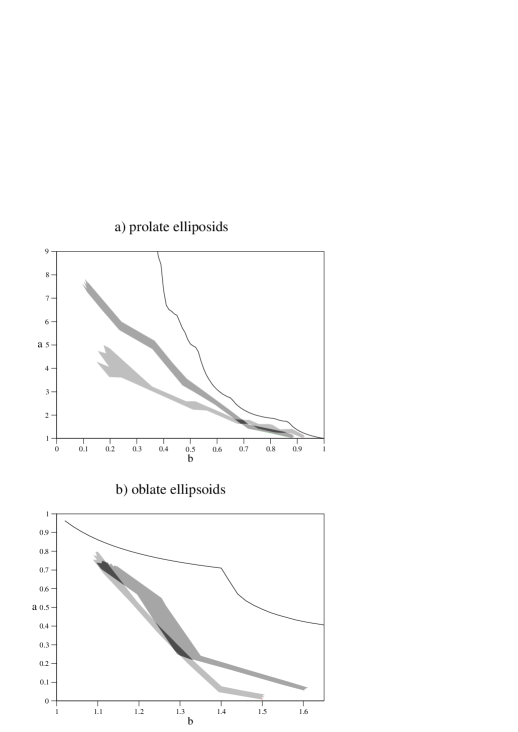
Figure 2: Phase diagrams for a) prolate and b) oblate hard ellipsoids of revolution on a simple cubic lattice. Solid lines refer to the closest packing for parallel ellipsoids. Within the light grey areas an order-disorder phase transition occurs, while the medium grey areas indicate where the numerical solution of the OZ/PY equations starts to diverge. For a more detailed discussion see text of Secs. IV.1 and IV.2.

IV.2 Numerical solution of the OZ equation using the PY approximation

In App. E, we show that the correct static structure factors $S_{\lambda\lambda^{\prime}}({\bf q})$, even for $K\subset S^{2}$, can be obtained by solving the OZ/PY equations for $\Omega,\Omega^{\prime}\in S^{2}$. We have chosen this option since it avoids the use of the projectors $R^{K}$ and $P^{K}$ (cf. Sec. III.2 and App. B). We also solved both equations for $\Omega,\Omega^{\prime}\in K$ as described in Sec. III.2, but it turned out that the results are worse. The reason is probably the fact that the cut-off $l_{max}$, at which the matrix equations are truncated, leads to a rather crude approximation for $R^{K}$ and $P^{K}$. For example, some of the truncated projectors are significantly non-idempotent.

The numerical solution of the OZ/PY equations is performed by the iterative procedure described below usually for lattices of size $32\times 32\times 32$, periodic boundary conditions and $l_{\text{max}}=4$. The correlation function matrices ${\bf G}_{xyz}\equiv{\bf G}_{{\bf x}_{nn^{\prime}}}\equiv{\bf G}_{nn^{\prime}}$ have, by symmetry and periodicity, only to be tabulated for $0\leq x\leq y\leq z\leq 16$, and the same for the discrete Fourier transformed matrices ${\bf S}({\bf q})$.

For some systems characterized by $(a,b)$, we have solved the OZ/PY equations additionally for $l_{\text{max}}=2$ and $l_{\text{max}}=6$. All the correlators we have investigated explicitely remain qualitatively unchanged, while the correlation lengths of these correlators become larger for increasing $l_{max}$. For some of the systems showing no convergence of the iteration scheme because of diverging correlation lengths for $l_{\text{max}}=4$ and $32\times 32\times 32$ lattice sites, system sizes up to $128\times 128\times 128$ have been used, but for none of these bigger system sizes convergence could be achieved.

After each numerical inversion or Fourier transform the symmetries are checked to be within certain error margins, and then each matrix is subjected to every symmetry operation under which it must be invariant. From all these symmetry-transformed matrices the average is calculated to rule out rounding errors to become too large.

Before starting the iterative procedure, the input quantities are calculated:

(a) For each pair $(a,b)$ of ellipsoid axes, the $f$-function matrix elements $f^{r}_{ll^{\prime}m}$ in the $r$-frame C. G. Gray, K. E. Gubbins (1984) according to Eq. (76) have to be calculated for all even $l\leq l^{\prime}\leq 2\,l_{\text{max}}$ and $0\leq m\leq\text{max}(l,l^{\prime})$. By Eqs. (72), the remaining elements are obtained. Then, these are transformed back to the laboratory frame. For the numerical integration a $400\times 200\times 200$–grid has been used.

(b) The values $\langle\hat{Y}_{41}\rangle$, $\langle\hat{Y}_{61}\rangle$ and $\langle\hat{Y}_{81}\rangle$ are taken from the MC simulation for the same pair $(a,b)$ or an appropriate extrapolation beyond the MC cubic phase boundary, where needed. Then, Eqs. (II.2) yield the canonical averages of the spherical harmonics, which are coupled to give the matrices ${\bf d}$ and ${\bf D}$, due to Eqs. (66b) and (66c).

The iterative procedure is now as follows:

(a) As input for the OZ equation in the $n$-th iteration step, we use the matrices ${\bf c}^{(n)^{\prime}}_{xyz}$, which will be specified below. According to Eqs. (31b) and  (32b), the matrices ${\bf c}^{\circ,(n)^{\prime}}_{xyz}$ are obtained by just cancelling the first columns and rows. The matrix elements $c^{\circ,(n)^{\prime}}_{xyz,\lambda\lambda^{\prime}}$ are then calculated for $0\leq x,y,z<32$ and subsequently Fourier transformed to yield $c^{\circ,(n)^{\prime}}_{pqr,\lambda\lambda^{\prime}}$. As very first input we choose ${\bf c}^{(1)^{\prime}}_{xyz=0}={\bf 0}$, ${\bf c}^{(1)^{\prime}}_{xyz}={\bf f}_{xyz}$ otherwise.

(b) The matrices ${\bf h}^{\circ,(n)^{\prime}}_{pqr}$ in the $n$-th iteration step are calculated from

$${\bf h}^{\circ,(n)^{\prime}}_{pqr}=\left(\left({\bf 1}-\frac{1}{4\pi}{\bf c}^{\circ,(n)^{\prime}}_{pqr}{\bf D}\right)^{-1}_{\bf 1}\right)^{\circ}{\bf c}^{\circ,(n)^{\prime}}_{pqr}\,,\quad n\geq 1\,.$$ (59)

They generally will not fulfill the constraint ${\bf h}^{\circ,(n)^{\prime}}_{xyz=0}={\bf 0}$. Therefore, we define matrices ${\bf h}^{\circ,(n)}_{pqr}={\bf h}^{\circ,(n)^{\prime}}_{pqr}-{\bf h}^{\circ,(n)^{\prime}}_{xyz=0}$, which fulfill the constraint. Substituting ${\bf h}^{\circ,(n)}_{pqr}$ into the OZ equation yields matrices ${\bf c}^{\circ,(n)^{\prime\prime}}_{pqr}$, from which ${\bf c}^{\circ,(n)^{\prime\prime}}_{xyz=0}$ is obtained. Then the final $n$-th approximation of the direct correlation function is chosen to be

$${\bf c}^{(n)}_{xyz}=\left\{\begin{array}[]{cc}\alpha\,{\bf c}^{(n)^{\prime\prime}}_{xyz}+(1-\alpha)\,{\bf c}^{(n)^{\prime}}_{xyz}\,,&xyz=0\,,\\ {\bf c}^{(n)^{\prime}}_{xyz}\,,&\text{otherwise}\,.\end{array}\right.$$ (60)

Note that the self part of the direct correlation function can definitely be determined in the form $\circ$ only (see Eq. (50)). In Eq. (60), $0<\alpha<1$ is a mixing parameter.

(c) ${\bf h}^{\circ,(n)}_{xyz}$ is obtained from ${\bf h}^{\circ,(n)}_{pqr}$ by Fourier transform and Eq. (B) yields ${\bf h}^{(n)}_{xyz}$ for $xyz\neq 0$. Then, ${\bf g}^{(n)}_{xyz}$ can be calculated following App. B. Using Eq. (III.1), ${\bf g}^{(n)}_{xyz}$ and ${\bf c}^{(n)}_{xyz}$ for $xyz\neq 0$, one obtains new direct correlation function matrices, which are mixed to a fraction of $\alpha$ with the matrices ${\bf c}^{(n)}_{xyz}$ to give ${\bf c}^{(n+1)^{\prime}}_{xyz}$, while ${\bf c}^{(n+1)^{\prime}}_{xyz=0}={\bf c}^{(n)}_{xyz=0}$ is chosen.

This prodedure is repeated until a fix point for the matrices has been reached. Typically, $\alpha=0.1$ is chosen to avoid divergence. Convergence is assumed if all elements of ${\bf h}^{\circ,(n)^{\prime}}_{xyz=0}$ have submerged a certain treshold, which is chosen to be $10^{-13}$ times the maximum absolute value of any matrix element $h^{\circ,(n)^{\prime}}_{xyz,\lambda\lambda^{\prime}}$. Additionally, the average of all non-zero matrix elements of ${\bf c}^{(n+1)}_{xyz}-{\bf c}^{(n)}_{xyz}$ must be below $\alpha$ times a second treshold, which is calculated in the same manner as the $h$-treshold, but by taking also the $ll^{\prime}=0$ matrix elements into account. It is interesting that Eq. (50) cannot be used for the calculation of ${\bf c}^{\circ,(n)}_{xyz=0}$, since this always leads to a divergence.

After the iteration has converged, also Eq. (50) can be checked to be true. For some systems, only a mixing parameter of $\alpha=0.05$ or $\alpha=0.02$ leads to convergence. For some of these critical systems the mixing is not enough for the direct correlation function, but also the new total correlation function has to be accepted only to a fraction of $\alpha$. The medium grey areas in Figs. 2 are the areas where the iterative procedure above, for a mixing paramter $\alpha=0.02$ applied to both the new direct and the new total correlation functions, turns from convergent to divergent, or begins to yield unphysical negative diagonal structure factors (see the next section for explanation).

Finally, Eq. (38) is used to calculate the static structure factors.

IV.3 Numerical results for the correlation functions

Results obtained from the numerical solution of the OZ/PY equations and the MC simulations are presented in Figures 3-13 for five different pairs of $(a,b)$, including prolate and oblate ellipsoids. We have restricted the illustrations of correlators in direct and reciprocal space to the matrix elements $(l=l^{\prime}=2,m=m^{\prime}=0,1,2)$, $(l=2,l^{\prime}=4,m=m^{\prime}=0,1,2)$ and $(l=l^{\prime}=4,m=m^{\prime}=0,1,2,3,4)$.

Log-lin representations of the direct space orientational correlators $G_{xyz,\lambda\lambda^{\prime}}$ are shown along lattice directions of high symmetry, i.e. $(x,y,z)=n\,(0,0,1)$, $(x,y,z)=n\,(0,1,1)$ and $(x,y,z)=n\,(1,1,1)$ for $n=0,1,\ldots,8$ (part a) of Figs. 3-13). Along these directions, all $G_{xyz,\lambda\lambda^{\prime}}$ are real by the symmetries (27) for the chosen $\lambda\lambda^{\prime}$. Note that the PY/OZ results could in principle be displayed up to $n=16$ and that a step $\Delta n=1$ corresponds to different lengths in direct space, namely $1$, $\sqrt{2}$ and $\sqrt{3}$ for the different lattice directions. In these illustrations, the values $n$ are chosen as abscissas. For each $m=m^{\prime}$ and each lattice direction, a separate picture is provided and a logarithmic plotting has been chosen for positive and negative values of $G_{xyz,\lambda\lambda^{\prime}}$ separately, i.e. the negative values are presented as $-\log\,|G_{xyz,\lambda\lambda^{\prime}}|$. This plotting shows that the direct space correlations decay exponentially in most cases. The respective values of $xyz,\lambda\lambda^{\prime}$ are included, too. Note that the scatter of the MC data for some $\lambda\lambda^{\prime}$ and large enough values of $n$ is due to the error margins.

Similarly to direct space, only correlators $S_{\lambda\lambda^{\prime}}({\bf q})$ along highly symmetric reciprocal lattice directions are displayed, i.e. $(p,q,r)=\xi(0,0,\pi)$, $(p,q,r)=\xi(0,\pi,\pi)$ and $(p,q,r)=\xi(\pi,\pi,\pi)$ for $\xi=0\ldots 1$, which are the correlators from the Brillouin zone center to its edge in the respective direction (part b) of Figs. 3-13). In these figures, $\xi$ is chosen as abscissa and the curves for all three reciprocal lattice directions have been put into one illustration for each pair $\lambda\lambda^{\prime}$, which is included in each picture. The curves are distinguished by the symbols $\Delta$ ($(0,0,\pi)$-direction), $\Sigma$ ($(0,\pi,\pi)$-direction) and $\Lambda$ ($(\pi,\pi,\pi)$-direction). All $S_{\lambda\lambda^{\prime}}({\bf q})$ which are shown are real by the symmetries (28). Additionally, by Eq. (37), the diagonal elements $S_{2m2m}({\bf q})$ and $S_{4m4m}({\bf q})$ are positive. The numerically determined correlators $S_{\lambda\lambda^{\prime}}({\bf q})$ have been interpolated by cubic splines with the correct boundary condition of vanishing gradients for $\xi=0$ and $\xi=1$. Note the different scales of the illustrations for different $\lambda\lambda^{\prime}$.

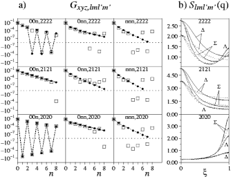
Figure 3: a) Log-lin-representation of the direct space orientational correlators $G_{xyz,2m2m}$ along highly symmetric lattice directions (solid circles = OZ/PY results, squares = MC results; dashed lines are a guide to the eye), b) orientational structure factors $S_{2m2m}({\bf q})$ along the respective reciprocal lattice directions (solid lines = OZ/PY results, dotted lines = MC results). These results are for oblate hard ellipsoids with axes $a=0.4$, $b=1.2$ on a sc lattice and $m=0,1,2$. For further explanation see text of Sec. IV.3.

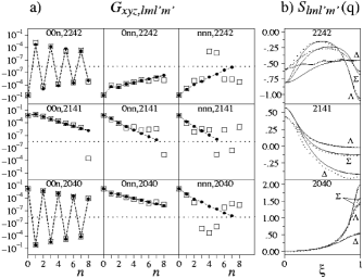
Figure 4: Same as Figure 3, but for $l=2$, $l^{\prime}=4$.

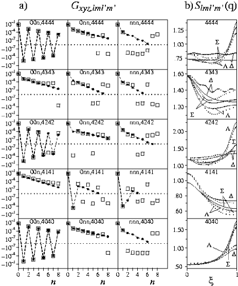
Figure 5: Same as Figure 3, but for $l=l^{\prime}=4$ and $m=0,1,2,3,4$.

Let us start by discussing the results shown in Figs. 3-5 for oblate hard ellipsoids with axes $a=0.4$ and $b=1.2$, corresponding to a packing fraction of $\phi\approx 0.3$. This system is quite close to the MC phase boundary shown in Fig. 2 b), but not close enough to find a tendency to a divergence of some of the $S_{\lambda\lambda^{\prime}}({\bf q})$. Notice the almost perfect agreement of the OZ/PY and MC orientational correlators in direct space, in case where the MC results are large enough. In fact, such an agreement appears for all investigated oblate ellipsoid systems, for which MC results are available, except for the system with $a=0.72$, $b=1.1$. Relatively long ranged oscillations appear for all correlators along the fourfold lattice direction $[0,0,1]$ having even $m=m^{\prime}$. The other correlators along the same direction decay faster and monotonously without oscillation, and also the correlators along the other directions decay without oscillations. Note that for $a=0.4$ and $b=1.2$ the ellipsoids can only interact via their nearest neighbours, which are localized along the fourfold lattice directions. Therefore, it is tempting to assume that the oscillations are primarily related to a direct particle interaction via nearest neighbours along a certain lattice direction. For denser oblate and some prolate systems, the oscillations extend up to many lattice constants, indicating the tendency to build up a medium range orientational order. For the structure factors $S_{\lambda\lambda^{\prime}}({\bf q})$, the agreement of OZ/PY and MC results is satisfactory. The most significant deviations appear for $l=l^{\prime}=2$ near ${\bf q}={\bf 0}$. The oscillations exhibited by some of the $G_{xyz,\lambda\lambda^{\prime}}$ manifest themselves in some maxima at the Brillouin zone edge, mainly for correlators $S_{2m2m}({\bf q})$ and $S_{4m4m}({\bf q})$ with $m$ even, but also for the correlators $S_{2040}({\bf q})$. Increasing $a$ and/or $b$ for oblate systems, the OZ/PY results for some of these zone-edge maxima show a tendency to diverge, accompanied by a simultaneous divergence mainly of the remaining $l=l^{\prime}=2$ correlators at the zone center.

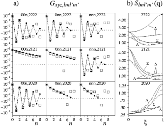
Figure 6: Same as Figure 3, but for prolate hard ellipsoids with axes $a=1.6$, $b=0.6$.

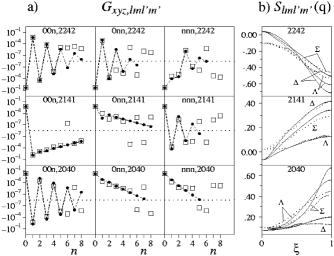
Figure 7: Same as Figure 3, but for $l=2$, $l^{\prime}=4$ and prolate hard ellipsoids with axes $a=1.6$, $b=0.6$.

Next, we have chosen the prolate ellipsoid system with axes $a=1.6$, $b=0.6$, having a packing fraction of $\phi\approx 0.3$, for which some results are shown in Figs. 6 and 7. For this system, oscillations appear additionally along the two other lattice directions (i.e. $[0,1,1]$ and $[1,1,1]$), which confirm the assumption that they may be caused by direct interaction via nearest neighbours for appropriate values of $b$ and not too large $a$. Again, the MC results in direct space match the analytical results very well, though latter overestimate some of the correlation lengths. This is clearly seen, for example, from the decrease of the correlators $G_{00n,2121}$ for increasing $n$, which is different for MC and OZ/PY results. The much too large OZ/PY results for the correlators $S_{2222}({\bf q})$ at the zone boundary along the $\Delta$-direction are perhaps also due to this overestimation. OZ/PY pretends an intersection of the curves for $S_{2040}({\bf q})$ along lattice directions $\Lambda$ and $\Sigma$ at $\xi\approx 0.8$, which is not present in the MC results. Note that the correlators $G_{0nn,2141}$ and $G_{nnn,2242}$ deviate significantly from the regular decrease inherent to other correlators.

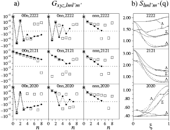
Figure 8: Same as Figure 3, but for prolate hard ellipsoids with axes $a=2.0$, $b=0.48$.

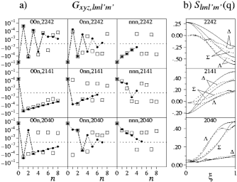
Figure 9: Same as Figure 3, but for $l=2$, $l^{\prime}=4$ and prolate hard ellipsoids with axes $a=2.0$, $b=0.48$.

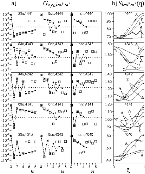
Figure 10: Same as Figure 3, but for $l=l^{\prime}=4$, $m=0,1,2,3,4$ and prolate hard ellipsoids with axes $a=2.0$, $b=0.48$.

Increasing $a$ to $2.0$ and decreasing $b$ to $0.48$ leads to $\phi\approx 0.24$ and the results of Figs. 8-10. Now, only one of the $l=l^{\prime}=2$ direct space correlators still shows pure oscillating behavior ($G_{0nn,2222}$), and also for the other values of $l,l^{\prime}$ the number of oscillating direct space correlators has decreased. Interestingly, some correlators oscillate for small values of $n$ and then start to decay monotonously (for example $G_{00n,2020}$, $G_{00n,2222}$, $G_{00n,2242}$), while others oscillate from $n=2$ on (for example $G_{0nn,2020}$, $G_{0nn,2040}$). Though not few of the direct space MC correlators differ by sign from the OZ/PY correlators (for example $G_{011,2121}$), the results still match satisfactory. Indeed, for some of the correlators $S_{4m4m}({\bf q})$ OZ/PY predicts crossings of the curves for different lattice directions, which are also present in the MC results. Coming back to the direct space orientational correlators, more and more of them have become non-regular functions of $n$, and also significant deviations from the almost exponential decay, which is present in many of the direct space correlators of the other systems discussed above, are encountered (see, e.g., $G_{0nn,2121}$). But the MC results for the correlators $G_{00n,4141}$, for example, prove that these non-regularities are not just an artefact of the analytical approach. Surprisingly, the OZ/PY correlator $G_{033,4141}\approx-2.97\times 10^{-9}$ is to small to be displayed in the pictures, though the surrounding correlators (i.e. $G_{0nn,4141}$, n = 0,1,2,4,5,6) clearly are not.

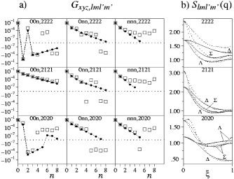
Figure 11: Same as Figure 3, but for prolate hard ellipsoids with axes $a=3.6$, $b=0.24$.

Now we pass to more and more elongated prolate ellipsoids and investigate what happens. In the limit of this process one obtains the hard-needle system, which is discussed, e.g., in C. Renner, H. Löwen, J. L. Barrat (1995). Ellipsoids with axes $a=3.6$ and $b=0.24$ have a huge aspect ratio of $X_{0}=\frac{a}{b}=15$. Of course, the packing fraction of these ellipsoids on the sc lattice is quite low, about $10\%$, but the frustration effect of the rigid lattice may provide completely new effects in comparison to a liquid. As shown in Fig. 11, the behavior of the correlators $G_{xyz,2m2m}$ is more regular in comparison to $a=2.0$ and $b=0.48$. Oscillations have disappeared completely. The OZ/PY results clearly underestimate the $S_{2m2m}({\bf q})$–correlators for small ${\bf q}$. This is also the case for the $S_{2m2m}({\bf q})$–correlators of all other investigated systems in the neighbourhood of $a=3.6$, $b=0.24$.

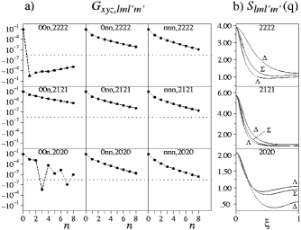
Figure 12: Same as Figure 3, but for prolate hard ellipsoids with axes $a=4.8$, $b=0.24$.

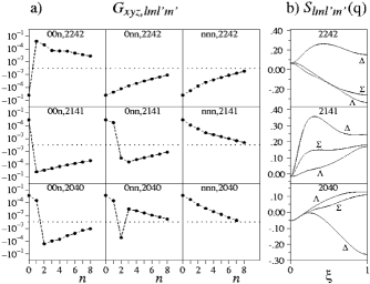
Figure 13: Same as Figure 3, but for $l=2$, $l^{\prime}=4$ and prolate hard ellipsoids with axes $a=4.8$, $b=0.24$.

The last system we present consists of ellipsoids of axes $a=4.8$ and $b=0.24$, for which it is $X_{0}=20$ and $\phi\approx 16\%$. The results of Figs. 12 and 13 belong to this pair $(a,b)$. The correlators in direct space essentially show up monotonous decay, and the correlation lengths have clearly increased in comparison to the elliposids of axes $a=3.6$ and $b=0.24$. Unfortunately, this system lies beyond the MC phase boundary (see Fig. 2a), so that no MC results are available. Despite of the monotonous behavior of most correlators, the $G_{00n,2020}$–correlators, for example, still show non-regular behavior, which vanishes for the most part switching to $a=5.6$ and $b=0.24$ (these results are not shown here). In Fig. 12, the beginning of a divergence of the $S_{2121}({\bf q}={\bf 0})$–correlator is seen, the corresponding value of the ($a=5.6,b=0.24$)-system being $\approx 20$. Also, what can be seen from Fig. 13, the $l=2$, $l^{\prime}=4$ correlators have got significant structure, and they seem not to diverge like the $l=l^{\prime}=2$ correlators.

V Discussion and conclusions

Our main goal has been the study of static orientational correlation functions for a molecular crystal in its disordered phase. For this, we have derived the OZ equation, well-known in liquid theory, for a rigid periodic lattice with internal orientational degrees of freedom. As a closure relation we have adopted the PY approximation. As pointed out, there are differences of the present approach to that for liquids. One of them is the fact that the OZ equation only involves the direct and total correlation functions $c^{\circ}_{nn^{\prime}}(\Omega,\Omega^{\prime})$ and $h^{\circ}_{nn^{\prime}}(\Omega,\Omega^{\prime})$, whereas the PY approximation relates $c_{nn^{\prime}}(\Omega,\Omega^{\prime})$ and $h_{nn^{\prime}}(\Omega,\Omega^{\prime})$. The functions with the superscript $\circ$ do not contain a constant part with respect to $\Omega$ or $\Omega^{\prime}$. Another important difference is the one-particle orientational distribution function $\rho^{(1)}(\Omega)$. In the isotropic phase of a molecular liquid it is $\rho^{(1)}(\Omega)=\frac{1}{4\pi}$, but due to the anisotropy of a crystal $\rho^{(1)}(\Omega)$ exhibits a nontrivial $\Omega$-dependence. In order to solve the OZ/PY equations, one has to calculate $\rho^{(1)}(\Omega)$ separately. In our case, we have performed MC simulations. Analytical approaches are also possible, e.g. for fixed $a$ one could perform a kind of virial expansion for small $b$.

Despite these differences, the form of the OZ equation for a molecular crystal is quite similar to that for molecular liquids C. G. Gray, K. E. Gubbins (1984). In order to explore the applicability of the lattice OZ equation in combination with the PY approximation, we have solved these equations for hard ellipsoids of revolution on a simple cubic lattice. Due to the orientational degrees of freedom, the orientational correlators $G_{nn^{\prime},\lambda\lambda^{\prime}}$ in direct space or $S_{\lambda\lambda^{\prime}}({\bf q})$ in reciprocal space, with $\lambda=(lm)$, are tensorial quantities. Accordingly, the self consistent numerical solution of the OZ/PY equations requires a truncation at $l_{\text{max}}$. We mainly have chosen $l_{\text{max}}=4$. As a result, we have found orientational correlators which have less structure in direct and reciprocal space than for liquid systems. Nevertheless, there are some interesting features depending on the length $a$ and $b$ of the ellipsoid axes. For oblate ellipsoids and prolate ones of large enough $b$, some of the direct space orientational correlators exhibit oscillations in certain lattice directions. Since the oscillations have period two they lead to maxima of $S_{\lambda\lambda^{\prime}}({\bf q})$ at the Brillouin zone edge for some $\lambda\lambda^{\prime}$. Although no long range orientational order exists, the oscillatory behavior originates from an alternating reordering of the ellipsoids on a finite length scale, which can extend up to many lattice constants.

Decreasing for prolate ellipsoids $b$ and increasing $a$ leads to a disappearance of almost all of these significant oscillations. In this case, the correlators $S_{2m2m}({\bf q})$ take their absolute maxima at the Brillouin zone center (cf. Figs. 11 and 12), indicating nematic-like fluctuations, while the same behavior is not found to the same extent for the other correlators (i.e. $S_{2m4m}({\bf q})$ (cf. Fig. 13) and $S_{4m4m}({\bf q})$ (cf. Fig. 10)). The behavior of the correlators $S_{2m2m}({\bf q})$ resembles a liquid of ellipsoids with aspect ratio larger than about two which forms a nematic phase D. Frenkel, B. M. Mulder, J. P. Mc Tague (1984). Surprisingly, increasing $a$ for fixed $b$ more and more the OZ/PY results for $S_{2m2m}({\bf q})$ lead to a divergence at ${\bf q}={\bf 0}$, which indicates the tendency to establish a long range nematic-like order. This finding demonstrates that PY theory can yield the onset of a phase transition to an ordered phase as it was already found before for a liquid of hard ellipsoids M. Letz, A. Latz (1999).

Some correlators for appropriately long prolate ellipsoids show up highly irregular behavior in direct space, which is nevertheless consistent with MC results (where available) and therefore has to be taken serious. We suppose the frustration effect of the lattice to be the reason for this non-regular behavior.

Comparison of the PY results with those from MC simulations shows a satisfactory agreement. But the quality of this agreement is less good as it is, e.g. for a liquid of hard spheres. The reason for this may lie in the PY approximation. For a liquid its physical content has been elucidated by Percus J. K. Percus (1962) (see also ref. J.-P. Hansen, I. R. McDonald (1990)) by use of a grand canonical ensemble. Since in a molecular crystal the particles are fixed, it is not obvious how this reasoning can be used. Of course, it might be interesting to investigate whether other closure relations J.-P. Hansen, I. R. McDonald (1990) or the turn to much higher $l_{\text{max}}$ can lead to an improvement.

To conclude, we have demonstrated that an extension of the OZ equation in combination with the PY approximation to molecular crystals leads to satisfactory results compared with MC data.

Appendix A Calculation of $h^{K}_{nn^{\prime}}(\Omega,\Omega^{\prime})$ from $h^{K,\circ}_{nn^{\prime}}(\Omega,\Omega^{\prime})$, $n\neq n^{\prime}$

In Apps. A-D, we discuss the most general case $K\subseteq S^{2}$. If $K=S^{2}$, the superscripts $K$ which are used have to be dropped to be consistent with the rest of the paper.

Using definiton (52), we have with Eq. (53a)

$$h^{K}_{nn^{\prime}}(\Omega,\Omega^{\prime})=h^{K,\circ}_{nn^{\prime}}(\Omega,\Omega^{\prime})+\frac{1}{|K|}\int\limits_{K}h^{K}_{nn^{\prime}}(\Omega,\Omega^{\prime})\,d\Omega+\frac{1}{|K|}\int\limits_{K}h^{K}_{nn^{\prime}}(\Omega,\Omega^{\prime})\,d\Omega^{\prime}-\frac{1}{|K|^{2}}\iint\limits_{KK}h^{K}_{nn^{\prime}}(\Omega,\Omega^{\prime})\,d\Omega\,d\Omega^{\prime}$$ (61)

If we take $\iint_{K}\rho^{(1)}(\Omega)\,\ldots\,\rho^{(1)}(\Omega^{\prime})\,d\Omega\,d\Omega^{\prime}$ on both sides of Eqs. (61), it remains due to Eqs. (15)

$$\frac{1}{|K|^{2}}\iint\limits_{KK}h^{K}_{nn^{\prime}}(\Omega,\Omega^{\prime})\,d\Omega\,d\Omega^{\prime}=\iint\limits_{KK}\rho^{(1)}(\Omega)\,h^{K,\circ}_{nn^{\prime}}(\Omega,\Omega^{\prime})\,\rho^{(1)}(\Omega^{\prime})\,d\Omega\,d\Omega^{\prime}\,.$$ (62)

Only $\int_{K}\ldots\,\rho^{(1)}(\Omega^{\prime})\,d\Omega^{\prime}$ applied to both sides of Eq. (61) yields

$$\frac{1}{|K|}\int\limits_{K}h^{K}_{nn^{\prime}}(\Omega,\Omega^{\prime})\,d\Omega^{\prime}=\frac{1}{|K|^{2}}\iint\limits_{KK}h^{K}_{nn^{\prime}}(\Omega,\Omega^{\prime})d\Omega\,d\Omega^{\prime}-\int\limits_{K}h^{K,\circ}_{nn^{\prime}}(\Omega,\Omega^{\prime})\,\rho^{(1)}(\Omega^{\prime})\,d\Omega^{\prime}$$ (63)

(analogously, $\int_{K}\rho^{(1)}(\Omega)\,\ldots\,d\Omega$ must be applied in the same manner). Then, (62) can be used with the first term on the rhs of (63), and finally we find that

$$h^{K}_{nn^{\prime}}(\Omega,\Omega^{\prime})=h^{K,\circ}_{nn^{\prime}}(\Omega,\Omega^{\prime})-\int\limits_{K}h^{K,\circ}_{nn^{\prime}}(\Omega,\Omega^{\prime})\,\rho^{(1)}(\Omega^{\prime})\,d\Omega^{\prime}-\int\limits_{K}\rho^{(1)}(\Omega)\,h^{K,\circ}_{nn^{\prime}}(\Omega,\Omega^{\prime})\,d\Omega$$

$$+ \iint\limits_{KK}\rho^{(1)}(\Omega)\,h^{K,\circ}_{nn^{\prime}}(\Omega,\Omega^{\prime})\,\rho^{(1)}(\Omega^{\prime})\,d\Omega\,d\Omega^{\prime}=\iint\limits_{KK}\left(\delta\,(\Omega|\Omega^{\prime\prime})-\rho^{(1)}(\Omega^{\prime\prime})\right)h^{K,\circ}_{nn^{\prime}}(\Omega^{\prime\prime},\Omega^{\prime\prime\prime})\left(\delta\,(\Omega^{\prime\prime\prime}|\Omega^{\prime})-\rho^{(1)}(\Omega^{\prime\prime\prime})\right)d\Omega^{\prime\prime}\,d\Omega^{\prime\prime\prime}\,.$$ (64)

Therefore, $h^{K}_{nn^{\prime}}(\Omega,\Omega^{\prime})$ is determined by $h^{K,\circ}_{nn^{\prime}}(\Omega,\Omega^{\prime})$ via Eq. (A). It is easy to prove that this $h^{K}_{nn^{\prime}}(\Omega,\Omega^{\prime})$ is the only one leading to the given $h^{K,\circ}_{nn^{\prime}}(\Omega,\Omega^{\prime})$ and simultaneously fulfilling Eqs. (15), i.e. $h^{\circ,K}_{nn^{\prime}}(\Omega,\Omega^{\prime})$ determines $h^{K}_{nn^{\prime}}(\Omega,\Omega^{\prime})$ uniquely.

Appendix B Calculation of the matrix elements $g^{K}_{nn^{\prime},\lambda\lambda^{\prime}}$, $n\neq n^{\prime}$

For the PY approximation in matrix form (III.1), the matrix elements $g^{K}_{nn^{\prime},\lambda\lambda^{\prime}}=1^{K}_{\lambda\lambda^{\prime}}+h^{K}_{nn^{\prime},\lambda\lambda^{\prime}}$ are needed. In the following, it is convenient to introduce the projection operator $P^{K}=(P^{K})^{2}=(P^{K})^{\dagger}$, defined on $S^{2}\times S^{2}$ as

$$P^{K}(\Omega,\Omega^{\prime}) = \left\{\begin{array}[]{c}\delta(\Omega|\Omega^{\prime})\,,\quad\Omega,\Omega^{\prime}\in K,\\ 0\,,\text{ otherwise}\end{array}\right.$$ (65c)

$$P^{K}_{\lambda\lambda^{\prime}} = i^{l^{\prime}-l}\int\limits_{K}Y_{\lambda}^{*}(\Omega)\,Y_{\lambda^{\prime}}(\Omega)\,d\Omega\,,$$ (65d)

and

$$d(\Omega,\Omega^{\prime}) =4\pi\,\rho^{(1)}(\Omega)\,\delta(\Omega|\Omega^{\prime})$$ (66a)

$$d_{\lambda\lambda^{\prime}} =4\pi\,i^{l^{\prime}-l}\int\limits_{K}\rho^{(1)}(\Omega)\,Y_{\lambda}^{*}(\Omega)\,Y_{\lambda^{\prime}}(\Omega)\,d\Omega.$$ (66b)

Using (66), the $$\lambda D(\Omega,\Omega^{\prime})$$ transform of (see Eq. (18)) can be represented as

$$D_{\lambda\lambda^{\prime}}=d_{\lambda\lambda^{\prime}}-d_{\lambda,00}\,d_{00,\lambda^{\prime}}$$ (66c)

Though defined on $S^{2}\times S^{2}$, $d=d^{K}$ can be assumed, since $d(\Omega,\Omega^{\prime})=0$ on $(S^{2}\times S^{2})\setminus(K\times K)$. The inverse function for $d$ on $K$ is $\frac{1}{4\pi}\frac{\delta(\Omega|\Omega^{\prime})}{\rho^{(1)}(\Omega)}$. Note that for $K=S^{2}$ one has $P^{S^{2}}_{\lambda\lambda^{\prime}}=\delta_{\lambda,00}\,\delta_{00,\lambda^{\prime}}$.

Now we calculate $g^{K}_{nn^{\prime},\lambda\lambda^{\prime}}$. First, the matrix elements $1^{K}_{\lambda\lambda^{\prime}}$ are given

$$1^{K}_{\lambda\lambda^{\prime}}=i^{l^{\prime}-l}\iint\limits_{KK}Y_{\lambda}^{*}(\Omega)\,Y_{\lambda^{\prime}}(\Omega^{\prime})\,d\Omega\,d\Omega^{\prime}=4\pi\,P^{K}_{\lambda,00}\,P^{K}_{00,\lambda^{\prime}}\,.$$ (67)

Next, Eq. (A) is used. The matrices ${\bf h}^{K,\circ}_{nn^{\prime}}$ are delivered by the OZ equation. According to (67), the matrix belonging to $\iint_{K}\rho^{(1)}(\Omega)\,h^{K,\circ}_{nn^{\prime}}(\Omega,\Omega^{\prime})\,\rho^{(1)}(\Omega^{\prime})\,d\Omega\,d\Omega^{\prime}$ is

$$\left(\iint\limits_{KK}\rho^{(1)}(\Omega)\,h^{K,\circ}_{nn^{\prime}}(\Omega,\Omega^{\prime})\,\rho^{(1)}(\Omega^{\prime})\,d\Omega\,d\Omega^{\prime}\right)_{\lambda\lambda^{\prime}}$$

$$=4\pi\,P^{K}_{\lambda,00}\,P^{K}_{00,\lambda^{\prime}}\iint\limits_{KK}\rho^{(1)}(\Omega)\,h^{K,\circ}_{nn^{\prime}}(\Omega,\Omega^{\prime})\,\rho^{(1)}(\Omega^{\prime})\,d\Omega\,d\Omega^{\prime}\,,$$ (68)

where by use of (66b) one easily computes that (using the summation rule)

$$\iint\limits_{KK}\rho^{(1)} (\Omega)\,h^{K,\circ}_{nn^{\prime}}(\Omega,\Omega^{\prime})\,\rho^{(1)}(\Omega^{\prime})\,d\Omega\,d\Omega^{\prime}$$

$$=\frac{1}{4\pi}\,d_{00,\lambda}\,h^{K,\circ}_{nn^{\prime},\lambda\lambda^{\prime}}\,d_{\lambda^{\prime},00}\,.$$ (69)

The matrix elements $(\int_{K}h^{K,\circ}_{nn^{\prime}}(\Omega,\Omega^{\prime})\,\rho^{(1)}(\Omega^{\prime})\,d\Omega^{\prime})_{\lambda\lambda^{\prime}}$ are also straightforward. Since the angular function depends not on $\Omega^{\prime}$, $\sqrt{4\pi}\,P^{K}_{00,\lambda^{\prime}}$ must occur, as in Eq. (67). The dependence on $\Omega$ and the integrals are represented by $\sqrt{4\pi}^{-1}\,h^{K,\circ}_{nn^{\prime},\lambda\lambda^{\prime\prime}}\,d_{\lambda^{\prime\prime},00}$, so that we finally have

$$\left(\int\limits_{K}h^{K,\circ}_{nn^{\prime}}(\Omega,\Omega^{\prime})\,\rho^{(1)}(\Omega^{\prime})\,d\Omega^{\prime}\right)_{\lambda\lambda^{\prime}}=h^{K,\circ}_{nn^{\prime},\lambda\lambda^{\prime\prime}}\,d_{\lambda^{\prime\prime},00}\,P^{K}_{00,\lambda^{\prime}}\,.$$ (70)

Altogether, the matrix elements $h^{K}_{nn^{\prime},\lambda\lambda^{\prime}}$, which must be completed by (67) to give $g^{K}_{nn^{\prime},\lambda\lambda^{\prime}}$, are

$$h^{K}_{nn^{\prime},\lambda\lambda^{\prime}} =h^{K,\circ}_{nn^{\prime},\lambda\lambda^{\prime}}-\,h^{K,\circ}_{nn^{\prime},\lambda\lambda^{\prime\prime}}\,d_{\lambda^{\prime\prime},00}\,P^{K}_{00,\lambda^{\prime}}-P^{K}_{\lambda,00}\,d_{00,\lambda^{\prime\prime}}\,h^{K,\circ}_{nn^{\prime},\lambda^{\prime\prime}\lambda^{\prime}}+P^{K}_{\lambda,00}\,d_{00,\lambda^{\prime\prime}}\,h^{K,\circ}_{nn^{\prime},\lambda^{\prime\prime}\lambda^{\prime\prime\prime}}\,d_{\lambda^{\prime\prime\prime},00}\,P^{K}_{00,\lambda^{\prime}}$$

$$=\left(P^{K}_{\lambda\lambda^{\prime\prime}}-P^{K}_{\lambda,00}d_{00,\lambda^{\prime\prime}}\right)h^{K,\circ}_{nn^{\prime},\lambda^{\prime\prime}\lambda^{\prime\prime\prime}}\left(P^{K}_{\lambda^{\prime\prime\prime}\lambda^{\prime}}-P^{K}_{00,\lambda^{\prime}}d_{\lambda^{\prime\prime\prime},00}\right)$$ (71)

Appendix C Calculation of $f^{K}_{nn^{\prime},\lambda\lambda^{\prime}}$, $n\neq n^{\prime}$

Contrary to the lattice correlation functions, $f_{nn^{\prime}}(\Omega,\Omega^{\prime})$ is not affected by the lattice and refers exclusively to what happens between two particles. Therefore, it is advantageous to use the $r$-frame for the calculation of the matrix elements, i.e. the coordinate system in which the connecting line of the particles coincides with the $z$-axis, and later to transform them back to the laboratory system. For $K=S^{2}$ in the $r$-frame, the matrix elements have similar properties as in R. Schilling, T. Scheidsteger (1997):

$$f^{r}_{nn^{\prime},lm,l^{\prime}m^{\prime}}=f^{r}_{nn^{\prime},ll^{\prime}m}\,\delta_{mm^{\prime}}\,,\quad\quad f^{r}_{nn^{\prime},ll^{\prime}m}=(-1)^{l+l^{\prime}}f^{r^{*}}_{nn^{\prime},ll^{\prime}m}\,,\quad\quad f^{r}_{nn^{\prime},ll^{\prime}m}=f^{r}_{nn^{\prime},ll^{\prime}-m}\,.$$ (72)

In the following, the abbreviation $Q_{lm}(\theta)=(-1)^{m}\left(\frac{2l+1}{4\pi}\right)^{\frac{1}{2}}\left(\frac{(l-m)!}{(l+m)!}\right)^{\frac{1}{2}}\sin\theta\,P_{lm}(\cos\theta)$ is used, where we define $P_{l,-m}(\cos\theta)=(-1)^{m}\frac{(l-m)!}{(l+m)!}\,P_{lm}(\cos\theta)$ to cover all possible values of $m$. Then it is

$$f^{r}_{nn^{\prime},ll^{\prime}m}=i^{l^{\prime}-l}\int\limits_{0}^{2\pi}\int\limits_{0}^{2\pi}\int\limits_{0}^{\pi}\int\limits_{0}^{\pi}f^{r}(|{\bf x}_{nn^{\prime}}|,\theta_{r},\theta_{r}^{\prime},\phi_{r}^{\prime}-\phi_{r})\,Q_{lm}(\theta_{r})\,Q_{l^{\prime}m}(\theta_{r}^{\prime})\,\text{e}^{im(\phi_{r}^{\prime}-\phi_{r})}\,d\theta_{r}\,d\theta_{r}^{\prime}\,d\phi_{r}\,d\phi_{r}^{\prime}$$ (73)

Switching to the new variables $\phi_{1}=\phi_{r}^{\prime}-\phi_{r}$ and $\phi_{2}=\phi_{r}^{\prime}+\phi_{r}$ brings about a functional determinant factor of $\frac{1}{2}$:

$$f^{r}_{nn^{\prime},ll^{\prime}m}=\frac{1}{2}\,i^{l^{\prime}-l}\int\limits_{0}^{4\pi}\int\limits_{-\Psi(\phi_{2})}^{\Psi(\phi_{2})}\int\limits_{0}^{\pi}\int\limits_{0}^{\pi}f^{r}(|{\bf x}_{nn^{\prime}}|,\theta_{r},\theta_{r}^{\prime},\phi_{1})\,Q_{lm}(\theta_{r})\,Q_{l^{\prime}m}(\theta_{r}^{\prime})\,\text{e}^{im\phi_{1}}\,d\theta_{r}\,d\theta_{r}^{\prime}\,d\phi_{1}\,d\phi_{2}\,,$$ (74)

where $\Psi(\phi_{2})=\phi_{2}$, $0\leq\phi_{2}\leq 2\pi$, $\Psi(\phi_{2})=4\pi-\phi_{2}$, $2\pi\leq\phi_{2}\leq 4\pi$. Now, the symmetries $f^{r}(|{\bf x}_{nn^{\prime}}|,\theta_{r},\theta_{r}^{\prime},\phi_{1})=f^{r}(|{\bf x}_{nn^{\prime}}|,\theta_{r},\theta_{r}^{\prime},-\phi_{1})=f^{r}(|{\bf x}_{nn^{\prime}}|,\theta_{r},\theta_{r}^{\prime},2\pi-\phi_{1})$ can be used:

$$f^{r}_{nn^{\prime},ll^{\prime}m} =i^{l^{\prime}-l}\int\limits_{0}^{4\pi}\int\limits_{0}^{\Psi(\phi_{2})}\underbrace{\int\limits_{0}^{\pi}\int\limits_{0}^{\pi}f^{r}(|{\bf x}_{nn^{\prime}}|,\theta_{r},\theta_{r}^{\prime},\phi_{1})\,Q_{lm}(\theta_{r})\,Q_{l^{\prime}m}(\theta_{r}^{\prime})\,\cos(m\phi_{1})\,d\theta_{r}\,d\theta_{r}^{\prime}\,}_{\circledast}d\phi_{1}\,d\phi_{2}$$

$$=2\,i^{l^{\prime}-l}\int\limits_{0}^{2\pi}\int\limits_{0}^{\phi_{2}}\circledast\;d\phi_{1}\,d\phi_{2}=2\,i^{l^{\prime}-l}\int\limits_{0}^{2\pi}\int\limits_{\phi_{1}}^{2\pi}\circledast\;d\phi_{2}\,d\phi_{1}=2\,i^{l^{\prime}-l}\int\limits_{0}^{2\pi}(2\pi-\phi_{1})\,\circledast\;d\phi_{1}=2\pi\,i^{l^{\prime}-l}\int\limits_{0}^{2\pi}\circledast\;d\phi_{1}$$

$$=4\pi\,i^{l^{\prime}-l}\int\limits_{0}^{\pi}\int\limits_{0}^{\pi}\int\limits_{0}^{\pi}f^{r}(|{\bf x}_{nn^{\prime}}|,\theta_{r},\theta_{r}^{\prime},\phi_{1})\,Q_{lm}(\theta_{r})\,Q_{l^{\prime}m}(\theta_{r}^{\prime})\,\cos(m\phi_{1})\,d\theta_{r}\,d\theta_{r}^{\prime}\,d\phi_{1}\,.$$ (75)

For particles of inversion symmetry, only the ($ll^{\prime}$ even) matrix elements do not vanish, and by using $f^{r}(|{\bf x}_{nn^{\prime}}|,\theta_{r},\theta_{r}^{\prime},\phi_{1})=f^{r}(|{\bf x}_{nn^{\prime}}|,\theta_{r},\pi-\theta_{r}^{\prime},\pi+\phi_{1})=\ldots$ for that case we find that

$$f^{r}_{nn^{\prime},ll^{\prime}m}=16\pi\,i^{l^{\prime}-l}\int\limits_{0}^{\pi}\int\limits_{0}^{\frac{\pi}{2}}\int\limits_{0}^{\frac{\pi}{2}}f^{r}(|{\bf x}_{nn^{\prime}}|,\theta_{r},\theta_{r}^{\prime},\phi_{1})\,Q_{lm}(\theta_{r})\,Q_{l^{\prime}m}(\theta_{r}^{\prime})\,\cos(m\phi_{1})\,d\theta_{r}\,d\theta_{r}^{\prime}\,d\phi_{1}\,.$$ (76)

Finally, having transformed back to the laboratory frame and the matrix elements $f_{nn^{\prime},\lambda\lambda^{\prime}}$ in hand, they can be projected due to ${\bf f}^{K}_{nn^{\prime}}={\bf P}^{K}\,{\bf f}_{nn^{\prime}}\,{\bf P}^{K}$.

Appendix D Calculation of $c^{K}_{nn^{\prime}}(\Omega,\Omega^{\prime})$, $n\neq n^{\prime}$, for hard particles

The appendices D and E are given in terms of angular functions only. The discussion in terms of matrices is much more complicated.

For hard particles, the values of $c^{K}_{nn^{\prime}}(\Omega,\Omega^{\prime})$ in the areas of overlap remain undetermined by Eq. (45), and the question arises if these values are also uniquely determined by $c^{K,\circ}_{nn^{\prime}}(\Omega,\Omega^{\prime})$. That this indeed is true will be proven below.

Most important for the following considerations is that no space angle $\Omega^{\prime}_{0}\in K$ can be found for which the pair $(n\Omega,n^{\prime}\Omega^{\prime}_{0})$ has overlap for all $\Omega\in K$. Otherwise, it would be $\Omega^{\prime}_{0}\notin K$. Note that, contrary to the case of overlap, for appropriate size of the particles and special values of $\Omega^{\prime}_{0}\in K$, the pair $(n\Omega,n^{\prime}\Omega^{\prime}_{0})$ has no overlap for all $\Omega\in K$. Given a solution $c^{K}_{nn^{\prime}}(\Omega,\Omega^{\prime})$ for which $c^{K,\circ}_{nn^{\prime}}(\Omega,\Omega^{\prime})=(R^{K}\,c^{K}_{nn^{\prime}}\,R^{K})(\Omega,\Omega^{\prime})$, it is $c^{K}_{nn^{\prime}}(\Omega,\Omega^{\prime})=0$, if $(n\Omega,n^{\prime}\Omega^{\prime})$ has no overlap. Eqs. (52), (53a) and the symmetries of the correlation functions given in Sec. II.2 show that

$$c^{K}_{nn^{\prime}}(\Omega,\Omega^{\prime})=c^{K,\circ}_{nn^{\prime}}(\Omega,\Omega^{\prime})+\hat{c}^{K}_{nn^{\prime}}(\Omega)+\hat{c}^{K}_{n^{\prime}n}(\Omega^{\prime})-\hat{c}^{K}_{nn^{\prime}}\,.$$ (77)

Let us fix $\Omega^{\prime}=\Omega^{\prime}_{1}\in K$ and let $K(\Omega^{\prime}_{1})\subset K$ be the area such that $(n\Omega,n^{\prime}\Omega^{\prime}_{1})$ has no overlap for all $\Omega\in K(\Omega^{\prime}_{1})$. Then it follows from Eq. (77)

$$\hat{c}^{K}_{nn^{\prime}}(\Omega)=-c^{K,\circ}_{nn^{\prime}}(\Omega,\Omega^{\prime}_{1})-\hat{c}^{K}_{n^{\prime}n}(\Omega^{\prime}_{1})+\hat{c}^{K}_{nn^{\prime}}\,.$$ (78)

for all $\Omega\in K(\Omega^{\prime}_{1})$, because of $c^{K}_{nn^{\prime}}(\Omega,,\Omega^{\prime}_{1})=0$. Since $c^{K,\circ}_{nn^{\prime}}(\Omega,\Omega^{\prime}_{1})$ is known, we have found $\hat{c}^{K}_{nn^{\prime}}(\Omega)$ on $K(\Omega^{\prime}_{1})$ up to a constant depending on $\Omega^{\prime}_{1}$. Next we choose $\Omega^{\prime}=\Omega^{\prime}_{2}\in K$ and $\Omega^{\prime}_{2}\neq\Omega^{\prime}_{1}$. Then $\hat{c}^{K}_{nn^{\prime}}(\Omega)$ is obtained for $\Omega\in K(\Omega^{\prime}_{2})$ up to a constant depending on $\Omega^{\prime}_{2}$. This can be continued by choosing $\Omega^{\prime}_{i}$, $i=1,2,\ldots,M$ such that $\cup_{i}\,K(\Omega^{\prime}_{i})=K$. In that case one can construct $\hat{c}^{K}_{nn^{\prime}}(\Omega)$ on $K$, for example in the form $\hat{c}^{\circ,K}_{nn^{\prime}}(\Omega)$ having vanishing constant part. The same is done for $\hat{c}^{\circ,K}_{n^{\prime}n}(\Omega^{\prime})$. Finally, we have

$$c^{K}_{nn^{\prime}}(\Omega,\Omega^{\prime})=c^{K,\circ}_{nn^{\prime}}(\Omega,\Omega^{\prime})+\hat{c}^{K,\circ}_{nn^{\prime}}(\Omega)+\hat{c}^{K,\circ}_{n^{\prime}n}(\Omega^{\prime})-\hat{\hat{c}}^{K}_{nn^{\prime}}\,,$$ (79)

where $\hat{\hat{c}}^{K}_{nn^{\prime}}$ follows immediately if (79) is used with any $\Omega,\Omega^{\prime}$ such that $(n\Omega,n^{\prime}\Omega^{\prime})$ has no overlap.

Appendix E Some remarks on how the case $K\subset S^{2}$ can be treated

In this appendix, we want to answer two questions concerning the case of hard core particles, whose geometry leads to $K\subset S^{2}$. First, assuming finite interaction if the “hard cores” of such particles overlap, i.e.

$$V_{nn^{\prime}}(\Omega,\Omega^{\prime})=V<\infty\,\text{ (overlap)}\,,$$ (80)

what happens to the solutions $h^{V}_{nn^{\prime}}(\Omega,\Omega^{\prime})$ and $c^{V}_{nn^{\prime}}(\Omega,\Omega^{\prime})$ of the OZ/PY equations (43a) and (44), together with Eqs. (A) and (32a), which are defined on $S^{2}\times S^{2}$, if we take the limit $V\longrightarrow\infty\,$? Second, does a $S^{2}\times S^{2}$-solution $h^{\infty}_{nn^{\prime}}(\Omega,\Omega^{\prime})$ and $c^{\infty}_{nn^{\prime}}(\Omega,\Omega^{\prime})$ of the OZ/PY equations for $V=\infty$ lead to the same static structure factors as the solution $h^{K}_{nn^{\prime}}(\Omega,\Omega^{\prime})$ and $c^{K}_{nn^{\prime}}(\Omega,\Omega^{\prime})$ of Sec. III.2?

The first question can be answered using the fact that the function $D^{V}(\Omega,\Omega^{\prime})$ (cf. Eq. (18)) and the Mayer function Eq. (45) behave continuously if we take the limit $V\longrightarrow\infty$:

$$\lim_{V\to\infty}D^{V}(\Omega,\Omega^{\prime}) =D^{\infty}(\Omega,\Omega^{\prime})$$ (81a)

$$\lim_{V\to\infty}f_{nn^{\prime}}^{V}(\Omega,\Omega^{\prime}) =f_{nn^{\prime}}^{\infty}(\Omega,\Omega^{\prime})$$ (81b)

This is true for $D^{V}(\Omega,\Omega^{\prime})$ since the one-particle density $\rho^{(1)}(\Omega)$ varies continuously with $V$. If also all other functions exist in the limit $V=\infty$ and if the limit interchanges with integration, we can write down Eqs. (43a), (44), (A) and (32a) including the functions $h^{V}_{nn^{\prime}}(\Omega,\Omega^{\prime})$, $h^{V,\circ}_{nn^{\prime}}(\Omega,\Omega^{\prime})$, $c^{V}_{nn^{\prime}}(\Omega,\Omega^{\prime})$, $c^{V,\circ}_{nn^{\prime}}(\Omega,\Omega^{\prime})$, $D^{V}(\Omega,\Omega^{\prime})$ and $f^{V}_{nn^{\prime}}(\Omega,\Omega^{\prime})$ for $V<\infty$ and take this limit. Then it is easy to see that the limiting direct and total correlation functions are a set of functions $h^{\infty}_{nn^{\prime}}(\Omega,\Omega^{\prime})$, $c^{\infty}_{nn^{\prime}}(\Omega,\Omega^{\prime})$, i.e. they solve the OZ/PY equations for $V=\infty$ on $S^{2}\times S^{2}$. Note that, as $h^{V}_{nn^{\prime}}(\Omega,\Omega^{\prime})$, $h^{\infty}_{nn^{\prime}}(\Omega,\Omega^{\prime})$ fulfills the constraints given by Eqs. (15).

Now we investigate if a solution $h^{\infty}_{nn^{\prime}}(\Omega,\Omega^{\prime})$ and $c^{\infty}_{nn^{\prime}}(\Omega,\Omega^{\prime})$ leads to the correct static structure factors Eqs. (37), (38) for $V=\infty$. For this, since $D^{\infty}(\Omega,\Omega^{\prime})=(D^{\infty}\,R^{K})(\Omega,\Omega^{\prime})=(R^{K}\,D^{\infty})(\Omega,\Omega^{\prime})=(R^{K}\,D^{\infty}\,R^{K})(\Omega,\Omega^{\prime})$, with $R^{K}(\Omega,\Omega^{\prime})$ due to Eq. (53), we have to prove that $(R^{K}\,h^{\infty,\circ}_{nn^{\prime}}\,R^{K})(\Omega,\Omega^{\prime})=h^{K,\circ}_{nn^{\prime}}(\Omega,\Omega^{\prime})$, $\Omega,\Omega^{\prime}\in K$, where the former symbol $\circ$ refers to removed constant parts with respect to $S^{2}$ and the latter with respect to $K$. This can be done as follows.

a) It is tempting to assume that the functions $h^{\infty}_{nn^{\prime}}(\Omega,\Omega^{\prime})$ and $c^{\infty}_{nn^{\prime}}(\Omega,\Omega^{\prime})$ restricted to $K$ match the functions $h^{K}_{nn^{\prime}}(\Omega,\Omega^{\prime})$ and $c^{K}_{nn^{\prime}}(\Omega,\Omega^{\prime})$ of Sec. III.2. Then, the PY approximation (44) restricted to $K$ is fulfilled trivially. Additionaly, the restricted function $h^{\infty}_{nn^{\prime}}(\Omega,\Omega^{\prime})$ fulfills the constraints of Eqs. (15) (rewritten for $K$ instead of $S^{2}$), since these integrals do not change if one restricts the integration domains to $K$ (because of $\rho^{(1)}(\Omega)=0$ on $\bar{K}$).

b) Because of

$$\int\limits_{K} \left(\delta(\Omega|\Omega^{\prime})-\frac{1}{K}\right)\left\{\int\limits_{S^{2}}\left(\delta(\Omega^{\prime}|\Omega^{\prime\prime})-\frac{1}{4\pi}\right)f(\Omega^{\prime\prime})\,d\Omega^{\prime\prime}\right\}d\Omega^{\prime}$$

$$=\int\limits_{K}\left(\delta(\Omega|\Omega^{\prime})-\frac{1}{K}\right)f(\Omega^{\prime})\,d\Omega^{\prime}$$ (82)

is the removal of the constant parts of a function with respect to $S^{2}$ and a subsequent restriction to $K$ and removal of the constant parts with respect to $K$ equivalent to restricting the function to $K$ first and then to remove the constant parts with respect to $K$.

c) Next we notice that the OZ equation (43a) for $S^{2}\times S^{2}$ decouples for $V=\infty$ on $K\times K$ completely from $\bar{K}$, as does the OZ equation of Sec. III.2.

d) If we write down this decoupled OZ equation with its solution $h^{\infty,\circ}_{nn^{\prime}}(\Omega,\Omega^{\prime})$ and $c^{\infty,\circ}_{nn^{\prime}}(\Omega,\Omega^{\prime})$, restrict it to $K\times K$ and apply the projection operator $R^{K}(\Omega,\Omega^{\prime})$ from both sides, it involves the functions $(R^{K}\,h^{\infty,\circ}_{nn^{\prime}}\,R^{K})(\Omega,\Omega^{\prime})$ and $(R^{K}\,c^{\infty,\circ}_{nn^{\prime}}\,R^{K})(\Omega,\Omega^{\prime})$. Due to b), this is the OZ equation on $K\times K$, written with the functions $h^{\infty}_{nn^{\prime}}(\Omega,\Omega^{\prime})$ and $c^{\infty}_{nn^{\prime}}(\Omega,\Omega^{\prime})$, which are restricted to $K$ and have removed constant parts with respect to $K$.

Now we have shown that the initial assumption made in a) was right. Therefore, to solve the OZ/PY equations for the case $K\subset S^{2}$, one can solve these equations also on $S^{2}$ for $V=\infty$, since the irrelevant $\bar{K}$-parts of the involved functions are projected out. We have also made plausible that the limiting process from finite to hard core interaction leads to such a solution on $S^{2}$, and that therefore the structure factors behave continuously for $V\longrightarrow\infty$. This is exactly what one expects by intuition.

References

• J.-P. Hansen, I. R. McDonald (1990) J.-P. Hansen, I. R. McDonald, Theory of Simple Liquids (Academic Press, San Diego, 1990), reprint 2nd ed.
• C. G. Gray, K. E. Gubbins (1984) C. G. Gray, K. E. Gubbins, Theory of Molecular Fluids, vol. 1 (Clarendon Press, Oxford, 1984).
• J. Ram, R. C. Singh, Y. Singh (1994) J. Ram, R. C. Singh, Y. Singh, Phys. Rev. E 49, 5117 (1994).
• M. Letz, A. Latz (1999) M. Letz, A. Latz, Phys. Rev. E 60, 5865 (1999).
• J. D. Wright (2001) J. D. Wright, Molecular Crystals (Cambrigde University Press, Cambridge, 2001).
• J. N. Sherwood (1979) J. N. Sherwood, ed., The Plastically Crystalline State (John Wiley & Sons, Chichester, 1979).
• M. H. Müser (1998) M. H. Müser, Ferroelectrics 208, 293 (1998).
• R. M. Lynden-Bell, K. H. Michel (1994) R. M. Lynden-Bell, K. H. Michel, Rev. Mod. Phys. 66, 721 (1994).
• M. Yvinec, R. Pick (1980) M. Yvinec, R. Pick, J. Physique 41, 1045, 1053 (1980).
• W. Breymann, R. Pick (1988) W. Breymann, R. Pick, Europhys. Lett. 6, 227 (1988).
• W. Breymann, R. Pick (1989) W. Breymann, R. Pick, J. Chem. Phys. 91, 3119 (1989).
• W. Breymann, R. Pick (1994) W. Breymann, R. Pick, J. Chem. Phys. 100, 2232 (1994).
• R. Schilling, T. Scheidsteger (1997) R. Schilling, T. Scheidsteger, Phys. Rev. E 56, 2932 (1997).
• T. Franosch, M. Fuchs, W. Götze, M. R. Mayr, A. P. Singh (1997) T. Franosch, M. Fuchs, W. Götze, M. R. Mayr, A. P. Singh, Phys. Rev. E 56, 5659 (1997).
• F. C. von der Lage, H. A. Bethe (1947) F. C. von der Lage, H. A. Bethe, Phys. Rev. 71, 612 (1947).
• J. Vieillard-Baron (1972) J. Vieillard-Baron, J. Chem. Phys. 56, 4729 (1972).
• A. Saupe (1964) A. Saupe, Z. Naturforsch. A 19A, 161 (1964).
• C. Renner, H. Löwen, J. L. Barrat (1995) C. Renner, H. Löwen, J. L. Barrat, Phys. Rev. E 52, 5091 (1995).
• D. Frenkel, B. M. Mulder, J. P. Mc Tague (1984) D. Frenkel, B. M. Mulder, J. P. Mc Tague, Phys. Rev. Lett. 52, 287 (1984).
• J. K. Percus (1962) J. K. Percus, Phys. Rev. Lett. 8, 462 (1962).