Critical properties of an aperiodic model for interacting polymers

Abstract

We investigate the effects of aperiodic interactions on the critical behavior of an interacting two-polymer model on hierarchical lattices (equivalent to the Migadal-Kadanoff approximation for the model on Bravais lattices), via renormalization-group and tranfer-matrix calculations. The exact renormalization-group recursion relations always present a symmetric fixed point, associated with the critical behavior of the underlying uniform model. If the aperiodic interactions, defined by s ubstitution rules, lead to relevant geometric fluctuations, this fixed point becomes fully unstable, giving rise to novel attractors of different nature. We present an explicit example in which this new attractor is a two-cycle, with critical indices different from the uniform model. In case of the four-letter Rudin-Shapiro substitution rule, we find a surprising closed curve whose points are attractors of period two, associated with a marginal operator. Nevertheless, a scaling analysis indicates that this attractor may lead to a new critical universality class. In order to provide an independent confirmation of the scaling results, we turn to a direct thermodynamic calculation of the specific-heat exponent. The thermodynamic free energy is obtained from a transfer matrix formalism, which had been previously introduced for spin systems, and is now extended to the two-polymer model with aperiodic interactions.

1 Introduction

In some recent publications [1]-[4], we have used renormalization-group (RG) and transfer-matrix (TM) techniques to investigate the effects of aperiodically distributed (but not disordered) interactions on the critical behavior of ferromagnetic spin models. In a real-space renormalization calculation for simple hierarchical structures, we have written exact recursion relations in order to show that relevant geometric (aperiodic) fluctuations play a very similar role to disorder. These calculations lead to the formulation of an exact extension for deterministic, aperiodic interactions of the well-known Harris criterion for the relevance of disorder [5], in a form coincident with Luck’s heuristic, general derivation of this extension [6]. Also, we have shown that relevant geometric fluctuations give rise to distinct critical exponents, associated with the appearance of new attractors in parameter space. The independent transfer-matrix calculations have confirmed these results and provided deeper insight on more refined details of the thermodynamics of aperiodic spin systems, such as log-periodic oscillations of thermodynamic functions.

Now we consider a model of two directed polymers on a diamond hierarchical lattice, with an aperiodic, layered distribution of interaction energies, according to various substitution rules (see [7, 8] for extensive reviews of substitution sequences and their applications to statistical models). Although the qualitative description of the critical behavior is essentially similar, the exact renormalization-group recursion relations in parameter space turn out to be much simpler as compared to the calculations for spin systems. The case of two-letter substitution rules is particularly simple. For irrelevant geometric fluctuations, the critical behavior is governed by a symmetric fixed point, with no changes with respect to the uniform case. For relevant fluctuations, we show that this symmetric fixed point becomes fully unstable, and the critical behavior is associated with a novel two-cycle attractor of saddle-point character. However, for more complex substitution rules, such as the Rudin-Shapiro sequence of four letters (which is known to mimic Gaussian random fluctuations in a sense [8]) there appears a surprisingly rich structure in the four-dimensional parameter space. Besides the expected symmetric fixed point, there are non-diagonal fixed points and continuous lines of two-cycle attractors, associated with a marginal operator, which might give rise to non-universal critical exponents. A scaling analysis indicates that this structure is responsible for a novel critical universality class. In order to check these results, we resorted to an independent thermodynamic calculation, on the basis of a transfer matrix scheme.

The layout of this paper is as follows. In Section 2, we define the polymer model, and present some renormalization-group calculations for two- and four-letter (Rudin-Shapiro) substitution rules. We show the existence of some surprising structures in parameter space, and, in particular, discuss a number of scaling results for the critical behavior. We then proceed to formulate an extension of the transfer matrix scheme for a two-polymer model. Although this technique has already been used for spin systems, its extension for this new situation requires a considerable amount of analytical work, as described in Sections 4 and 5. In Section 3, we just formulate the transfer-matrix scheme for a two-polymer model. In Section 4, we study in great detail the algebraic structure of the transfer matrices, in order to unveil, in Section 5, the existence of a recursion relation for the eigenvalues of the transfer matrices associated with two successive generations of the hierarchical structure. In Section 6, we use the recursion relations in order to write down explicit thermodynamic functions. In Section 7 we present the results for aperiodic models, which are compared to the renormalization-group predictions.

2 The interacting polymer model

The binding-unbinding phase transition in a disordered model of two directed and interacting polymers on a hierarchical lattice has been investigated by Mukherji and Bhattacharjee [9], and we follow these authors on the definition of the model. We simply place two directed polymers on a diamond hierarchical. They start at one end of the lattice and stretch continuously to the other end (the root sites). There is an attractive interaction, $-\epsilon$, whenever a bond of the lattice is shared by a monomer of each polymer. This energy can be made to depend on the position of the bond along a branch, in a random or deterministic fashion. Note that, although seemingly artificial, the model is nothing else than a bona-fide Migdal-Kadanoff approximation for the same interacting problem on a genuine Bravais lattice.

In the basic cell of a diamond lattice, with $q$ branches and $p$ bonds per branch, there are configurations of energy $-p\epsilon$, where the two polymers occupy the same $p$ bonds of a branch, and configurations of zero energy, where the polymers stretch along different branches. Using the Boltzmann factor $y=\exp\left(\beta\epsilon\right)$ and the combinatorial coefficient $C_{q}^{2}=q\left(q-1\right)/2$, it is easy to write the RG recursion relation

$$y^{\prime}=\frac{1}{q}y^{p}+\frac{q-1}{q}.$$ (1)

Taking $p=2$, for example, we see that besides the trivial fixed points, $y^{\ast}=1$ and $\infty$, associated with zero and infinite temperatures, there is a nontrivial fixed point, $y^{\ast}=q-1$, which is physically acceptable for $q>2$ (there is no phase transition on the simple diamond lattice with $q=2$ branches). Also, from the linearization of the recursion relation about the nontrivial fixed point, we have the thermal eigenvalue

$$\Lambda=\frac{2\left(q-1\right)}{q}.$$ (2)

In order to obtain the specific-heat exponent, $\alpha$, one should note that, as the polymers are one-dimensional objects, the thermodynamic extensivity of this model relates to the polymer length, instead of the volume. Thus, the important density is the free energy per monomer, which is assumed to behave according to the fundamental scaling relation

$$f\left(y^{\prime}\right)=pf\left(y\right).$$ (3)

From this relation, we have the critical exponent associated with the specific heat,

$$\alpha=2-\frac{\ln p}{\ln\Lambda}.$$ (4)

This quantity will be used to characterize the possible universality classes of the model, depending on $q$, $p$ and the presence of aperiodically distributed interactions.

Consider, for example, for $p=2$, a layered distribution of interactions [1], $\epsilon_{a}$ and $\epsilon_{b}$, chosen according to the two-letter period-doubling sequence,

$$a\rightarrow ab,\qquad b\rightarrow aa.$$ (5)

In Figure 1 we give an example of the construction of a simple diamond lattice with this kind of aperiodicity, starting from the letter $a$. Along each branch the interaction energies are distributed according to the letters of the aperiodic sequence generated by the recursive application of the rule. The same arguments as used in the last paragraph to derive Eq. (1) for the uniform case, lead to a pair of recursion relations,

$$y_{a}^{\prime}=\frac{1}{q}y_{a}y_{b}+\frac{q-1}{q},$$ (6)

and

$$y_{b}^{\prime}=\frac{1}{q}y_{a}^{2}+\frac{q-1}{q},$$ (7)

where $y_{a,b}=\exp\left(\beta\epsilon_{a,b}\right)$, and $\epsilon_{a,b}>0$ is the interaction energy at bonds of types $a$ and $b$, respectively. For $y_{a}=y_{b}=y$, we recover the recursion relation associated with the uniform model.

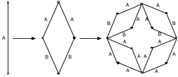
Figure 1: Initial stages of the construction of a Migdal-Kadanoff hierarchical lattice with $q=2$ branches and $p=2$ bonds per branch, and layered aperiodic interactions according to the period doubling rule, $a\rightarrow ab$, $b\rightarrow aa$ (letters $a$ and $b$ indicate the two possible values of the interaction energy, $\epsilon_{a}$ and $\epsilon_{b}$).

It is easy to see that, for $q>2$, there is no physically acceptable nontrivial fixed point, except the symmetric fixed point, $y_{a,b}^{\ast}=y^{\ast}=q-1$. The linearization of the recursion relations (6) and (7) in the neighborhood of this symmetric fixed point leads to the matrix form

$$\left(\begin{array}[]{c}\Delta y_{a}^{\prime}\\ \Delta y_{b}^{\prime}\end{array}\right)=\frac{y^{\ast}}{q}\left(\begin{array}[]{cc}1&1\\ 2&0\end{array}\right)\left(\begin{array}[]{c}\Delta y_{a}\\ \Delta y_{b}\end{array}\right),$$ (8)

with eigenvalues $\Lambda_{1}=2y^{\ast}/q=2\left(q-1\right)/q$, and $\Lambda_{2}=-y^{\ast}/q=-(q-1)/q$. Therefore, if $q>2$, we have $\Lambda_{1}>1$ and $\left|\Lambda_{2}\right|<1$, which shows that the geometric fluctuations are completely irrelevant in this case (since $\Lambda_{1}$ is the same eigenvalue associated with the non-trivial fixed point of the underlying uniform model, and the behavior is irrelevant along the other direction).

We now turn to a more interesting case. Consider a diamond lattice with $p=3$ bonds and $q$ branches. Suppose that the (layered) interactions are chosen according to a period-$3$ two-letter sequence, $a\rightarrow abb$ and $b\rightarrow aaa$. The new recursion relations are given by

$$y_{a}^{\prime}=\frac{1}{q}y_{a}y_{b}^{2}+\frac{q-1}{q},$$ (9)

and

$$y_{b}^{\prime}=\frac{1}{q}y_{a}^{3}+\frac{q-1}{q}.$$ (10)

For $q>3$, there is just a single nontrivial fixed point, at a symmetric location,

$$y_{a}^{\ast}=y_{b}^{\ast}=y^{\ast}=-\frac{1}{2}+\frac{1}{2}\sqrt{4q-3}.$$ (11)

The linearization in the neighborhood of this fixed point leads to the matrix equation

$$\left(\begin{array}[]{c}\Delta y_{a}^{\prime}\\ \Delta y_{b}^{\prime}\end{array}\right)=\frac{\left(y^{\ast}\right)^{2}}{q}\left(\begin{array}[]{cc}1&2\\ 3&0\end{array}\right)\left(\begin{array}[]{c}\Delta y_{a}\\ \Delta y_{b}\end{array}\right),$$ (12)

with eigenvalues

$$\Lambda_{1}=3\frac{y^{\ast 2}}{q}=\frac{3}{2q}\left[2q-1-\sqrt{4q-3}\right],$$ (13)

and

$$\Lambda_{2}=-2\frac{y^{\ast 2}}{q}=-\frac{1}{q}\left[2q-1-\sqrt{4q-3}\right].$$ (14)

For $3<q<3+\sqrt{5}$, it is easy to see that $\Lambda_{1}>1$, and $\left|\Lambda_{2}\right|<1$. As in the case of the simple diamond lattice with $p=2$ bonds, geometric fluctuations are irrelevant and the critical behavior is identical to the uniform case. However, for $q>3+\sqrt{5}=5.236068...$, we have $\left|\Lambda_{2}\right|>1$, and the symmetric fixed point becomes fully unstable, and, therefore, cannot be reached from arbitrary initial conditions (the values of $\epsilon_{a}$ and $\epsilon_{b}$). For example, for $q=5$, we have $y_{a}^{\ast}=y_{b}^{\ast}=y^{\ast}=1.561552...$, with eigenvalues $\Lambda_{1}=2.140568...$ and $\Lambda_{2}=0.951363...<1$. For $q=6$, however, we have $y_{a}^{\ast}=y_{b}^{\ast}=y^{\ast}=1.791287...$, with eigenvalues $\Lambda_{1}=2.573958...$ and $\Lambda_{2}=1.143981...>1$. But, as in the case of spin models on hierarchical lattices [2], there is a two-cycle in parameter space. It is easy to numerically locate this cycle at $\left(y_{a}^{\ast},y_{b}^{\ast}\right)=\left(1.419001...,2.267305...\right)$ and $\left(2.049103...,1.309541...\right)$, with eigenvalues of the linearized second iterate given by $\Lambda_{1}=2.624300...>1$ and $\Lambda_{2}=0.772598...<1$. A new critical universality class is therefore expected to be defined by this attractor.

The behavior in parameter space is much more interesting if we consider the Rudin-Shapiro, four-letter substitution rule, $a\rightarrow ac$, $b\rightarrow dc$, $c\rightarrow ab$, $d\rightarrow db$. Consider a simple diamond lattice with $p=2$ bonds and $q$ branches. It is straightforward to write four algebraic recursion relations,

$$y_{a}^{\prime}=y_{a}y_{c}/q+\left(q-1\right)/q,\qquad y_{b}^{\prime}=y_{d}y_{c}/q+\left(q-1\right)/q,$$ (15)

$$y_{c}^{\prime}=y_{a}y_{b}/q+\left(q-1\right)/q,\qquad y_{d}^{\prime}=y_{d}y_{b}/q+\left(q-1\right)/q,$$ (16)

which lead to the symmetric fixed point

$$y_{a}^{\ast}=y_{b}^{\ast}=y_{c}^{\ast}=y_{d}^{\ast}=y^{\ast}=q-1.$$ (17)

From the linearization about this fixed point, we have the eigenvalues

$$\Lambda_{1}=2\frac{q-1}{q},\quad\Lambda_{2}=\sqrt{2}\frac{q-1}{q},\quad\Lambda_{3}=-\sqrt{2}\frac{q-1}{q},\quad\Lambda_{4}=0.$$ (18)

The introduction of aperiodic interactions becomes relevant for the simple diamond lattice if $q>2+\sqrt{2}=3.41...$, which corresponds to $\left|\Lambda_{2}\right|=\left|\Lambda_{3}\right|>1$.

Recursion relations (15) and (16) are so simple that we can perform a number of detailed calculations. In particular, it is easy to show the existence of additional, non-diagonal fixed points, given by

$$y_{a,d}^{\ast}=\frac{1}{4\left(q-1\right)}\left[q\left(q^{2}-2q+2\right)\pm q\sqrt{\left(q^{2}-2\right)\left(q^{2}-4q+2\right)}\right],$$ (19)

$$y_{b,c}^{\ast}=q-\frac{q-1}{y_{d,a}^{\ast}}.$$ (20)

The Jacobian matrix associated with the linear form in the neighborhood of these fixed points can be written as

$$\frac{1}{q}\left(\begin{array}[]{cccc}y_{c}^{\ast}&0&y_{a}^{\ast}&0\\ 0&0&y_{d}^{\ast}&y_{c}^{\ast}\\ y_{b}^{\ast}&y_{a}^{\ast}&0&0\\ 0&y_{d}^{\ast}&0&y_{b}^{\ast}\end{array}\right).$$ (21)

Besides two trivial eigenvalues, $\Lambda_{3}=0$ and $\Lambda_{4}=-1$, there is an additional pair of eigenvalues ($\left|\Lambda_{1}\right|>1$ and $\left|\Lambda_{2}\right|<1$) given by the solutions of the quadratic equation

$$2q^{4}\Lambda^{2}-4q^{2}\left(q^{2}+q-1\right)\Lambda+q^{4}+8q^{3}-4q^{2}-8q+4=0.$$ (22)

As $\left|\Lambda_{4}\right|=1$, we have a typical case of marginal behavior, which cannot be analysed without resorting to higher-order calculations. However, the marginal operator does not give rise to a line of fixed points, as could be expected. Instead, with an additional algebraic effort, it is possible to show the existence of a continuous line whose points are two-cycles, by solving the polynomial equations

$$y_{a,b,c,d}=y_{a,b,c,d}^{\prime\prime}\left(y_{a},y_{b},y_{c},y_{d}\right),$$ (23)

where $y^{\prime\prime}$ is the second iterate of the recursion relations. Given any $q>2+\sqrt{2}$, these equations lead to a pair of one-parameter algebraic curves, which meet smoothly and form a single, non-intersecting closed curve, containing the non-diagonal fixed points. Any point belonging to this closed curve is mapped into another point on the curve upon one iteration of the recursion relations, and back to itself upon a further one. We have used algebraic computation to check this result very thoroughly. As an example, for $q=4$, we have the equations

$$y_{a}=3\frac{t+4}{4t-3},$$ (24)

$$y_{b}=-3\frac{70t^{2}+71t-114\pm g(t)}{t\left[6t^{2}-137t+78\pm g(t)\right]},$$ (25)

$$y_{c}=-\frac{6t^{2}-128t+114\pm g(t)}{3t\left(t+4\right)}$$ (26)

and

$$y_{d}=t,$$ (27)

with

$$g(t)=(36t^{4}-2220t^{3}+15529t^{2}-27132t+12296)^{1/2},$$ (28)

and the parameter $t$ taking values between $1.5142\ldots$ and $5.4112\ldots$. In Figure 2 we show a three-dimensional projection of this attractor. The linearization of the second iterates about any point of the curve leads to the eigenvalues $0$, $-1$, and a conjugate pair, $\left|\Lambda_{1}\right|>1$ and $\left|\Lambda_{2}\right|<1$ (the values of which do not depend on the point about which linearization is being carried out). The effects of the marginal eigenvalues on the specific-heat exponent, related to the existence of an extended attractor in parameter space, have to be checked very carefully, so we turn to the direct thermodynamic analysis of the free-energy singularity.

Figure 2: Three-dimensional projection of the attractor of the RG recursion relations for the Rudin-Shapiro aperiodic sequence, in a lattice with $p=2$ and $q=4$. The non-diagonal fixed points are shown as circles.

Before proceeding to the transfer-matrix calculations, however, it is worth remarking that, from a broad renormalization-group perspective, relevance and irrelevance of aperiodic distributions of couplings is related to the existence or not of a second eigenvalue with modulus larger than unity. The general structure of the recursion relations can be used to derive a relevance criterion which is ultimately based on the geometry of the lattice (that is, the values of $p$ and $q$), and some measure of the “strength” of the aperiodic fluctuations, such as the wandering exponent [6].

3 Transfer matrix formulation

One of us has successfully used a transfer matrix (TM) technique to obtain the thermodynamic properties of several spin models on fractal lattices [3, 4]. The essential step of this scheme consists in the derivation of maps relating the eigenvalues of the transfer matrices associated with two subsequent generations, $G$ and $G+1$. In a certain sense, this formalism is equivalent to a method used by Derrida et al. [10] to establish a map for the free energy, although it enables the calculation of a correlation length, which turns out to be very useful to locate the critical temperature (in spin systems).

In order to introduce the transfer matrix formulation, let us define the model in a mathematically more precise way. Again, we will consider a simple diamond hierarchical lattice (remembering that it has $q$ branches and $p$ bonds per branch in each basic cell). At a generation $G$ of the hierarchical construction, the lattice has $q^{G}$ branches, each of them formed by $p^{G}$ bonds. A polymer $A,$ extending from one root site to the other, is formed by $p^{G}$ connected monomers, and represented by a directed continuous path between the two root sites. A given monomer, labeled $i$ ($0\leq i\leq p^{G}-1$), occupies one of the $q^{G}$ available branches at the $i$th position along the path. We may define a numbering for the $q^{G}$ branches of the lattice, and let the variables $a_{i}$ indicate which one is occupied by the $i$th monomer; clearly, $1\leq a_{i}\leq q^{G}$, with analogous definitions for the other polymer, $B$. The two polymers interact at position $i$, with energy $-\epsilon_{i}<0$, if the $i$th monomers of the two distinct polymers occupy the same bond (note that the energy depends only on the position $i$, since we will consider layered interactions). If the $i$th monomers occupy distinct bonds, the interaction energy vanishes.

This definition of the two-polymer model can be summarized by the Hamiltonian

$$\mathcal{H}_{G}=-\sum_{i=0}^{p^{G}-1}\epsilon_{i}\delta\left(a_{i},b_{i}\right),$$ (29)

where $\delta\left(a_{i},b_{i}\right)$ indicates a Kronecker delta.

In Figure 3, we illustrate the simplest case, for $G=1$, $p=2$ and $q=2$. Note that, in fact, we are considering a periodic chain of $N$ hierarchical cells, each one grown up to generation $G$. For a single cell, as each monomer can independently occupy any of the $q$ branches, there are $q^{p}$ possible configurations for each position $i$ (remember that, as $p=2$, $i$ can have only two values in each cell), so that a total of $16$ possible states can be devised for this specific situation. However, we have to take into account that each polymer is required to form a continuous path between the root sites, so that several configurations have to be excluded. Formally, we may calculate the partition function including these forbidden configurations, if we introduce in the Hamiltonian an additional term of the form $\eta\sum_{i}V_{i}(a_{i},a_{i+1},b_{i},b_{i+1})$, with $\eta\rightarrow\infty$, such that $V_{i}=0$ for the acceptable configurations, and $V_{i}>0$ whenever $a_{i}$, $a_{i+1}$ and $b_{i}$, $b_{i+1}$ are not properly constrained. The explicit form of this potential is somewhat cumbersome, and will not be given here.

Figure 3: Periodic chain of $N$ hierarchical cells joined by the root sites, each consisting on the first generation of a diamond lattice with $p=2$ and $q=2$. This is the initial stage of the construction of the transfer-matrix formalism for the interacting polymer model.

Although it is straightforward to write a partition function for the particular case illustrated in Figure 3,

$$Z_{1}=\left(2e^{\beta\epsilon_{0}}e^{\beta\epsilon_{1}}+2\right)^{N},$$ (30)

the calculation of $Z_{G}$, for arbitrary values of $G$, and hence of the thermodynamic properties of the model, represents a much more difficult task. This is the reason to invoke the transfer matrix technique. However, this problem of interacting polymers, with interaction energies depending on monomer positions along the bonds, requires a completely new definition of the transfer matrices.

For the sake of simplicity, we restrict the presentation of the formalism to the homogeneous (uniform) system, which requires a smaller number of different types of elementary TM’s. It is straightforward to work out an extension for the more complex situation of a model with aperiodic interactions.

With the inclusion of the infinite-energy term, Eq. (29) can be written in the symmetrized form,

$$\mathcal{H}_{G}=-\frac{\epsilon}{2}\sum_{i=0}^{p^{G}-1}\left[\delta\left(a_{i},b_{i}\right)+\delta\left(a_{i+1},b_{i+1}\right)\right]+\eta\sum_{i=0}^{p^{G}-1}V_{i}\left(a_{i},a_{i+1},b_{i},b_{i+1}\right),$$ (31)

where we impose periodic boundary conditions, $a_{p^{G}}=a_{0}$ and $b_{p^{G}}=b_{0}$. Now we define the $q^{2G}\times q^{2G}$ matrices,

$$(\mathbf{M}_{G}^{(i)})_{a_{i}b_{i};a_{i+1}b_{i+1}}=\exp\left\{\frac{\beta\epsilon}{2}\left[\delta(a_{i},b_{i})+\delta(a_{i+1},b_{i+1})\right]+\beta\eta V_{i}(a_{i},a_{i+1},b_{i},b_{i+1})\right\},$$ (32)

and recall that the index $i$ ranges from $0$ to $p^{G}-1$ (the length of each polymer in generation $G$ is $p^{G}$ ). Also, it should be remarked that, in the double indices of $\mathbf{M}_{G}^{(i)}$, each term $a_{i}b_{i}$ must be interpreted as a tensor product of the variables $a_{i}$ and $b_{i}$, each of them taking $q^{G}$ independent values. The Boltzmann weights at each $\mathbf{M}_{G}^{(i)}$ relate to the attracting energy between two monomers and to whether the $i$th monomer, placed at the bond $a_{i}\left(b_{i}\right)$, can be linked to the $(i+1)$th monomer at the bond $a_{i+1}(b_{i+1})$, without violating the continuity constraint. The definition of the TM’s in Eq. (32) leads to the formal identification of the partition function with the trace of a product of TM’s,

$$Z_{G}=\Tr\prod_{i=0}^{p^{G}-1}\mathbf{M}_{G}^{(i)}\equiv\Tr\mathbf{M}_{G}.$$ (33)

Note that in this equation we considered $N=1$, since periodic boundary conditions have already been enforced.

In the following we will show that $\mathbf{M}_{G}$ has just one non-zero eigenvalue, which we call $\eta_{G}$, and which is obviously its trace. For the sake of clarity, we state now the result that $\eta_{G}$ is given by a recursion relation,

$$\eta_{G}=q\left[\eta_{G-1}^{2}+(q-1)\chi_{G-1}^{4}\right],$$ (34)

with

$$\chi_{G}=q^{\left(2^{G}-1\right)},$$ (35)

and $\eta_{0}=y^{2}$. The next two sections are devoted to the derivation of this result, and some readers may be interested on skipping directly to Section 6, where we establish recursion relations for the relevant thermodynamic functions.

4 Detailed structure of the matrices

The essential difficulty in the evaluation of $Z_{G}$ has been shifted into the calculation of the eigenvalues of a product of different kinds of TM’s, $\mathbf{M}_{G}^{(i)}.$ In order to emphasize the main ideas of the method, let us explore in greater detail the structure of the matrices in the case illustrated in Figure 3, where now the partition function is just the one given by Eq. (30), with $\epsilon_{1}=\epsilon_{2}$ (remember we are considering uniform interactions for the time being). Defining now $y=\exp\left(\beta\epsilon/2\right),$ we note that the TM’s $\mathbf{M}_{G=1}^{(i)}$ assume the two distinct forms,

$$\mathbf{M}_{1}^{(1)}=\left(\begin{array}[]{cccc}y^{2}&y&y^{2}&y\\ y&1&y&1\\ y^{2}&y&y^{2}&y\\ y&1&y&1\end{array}\right)=\left(\begin{array}[]{cc}1&1\\ 1&1\end{array}\right)\otimes\left(\begin{array}[]{cc}y^{2}&y\\ y&1\end{array}\right)\equiv\mathbf{L}_{1}^{(1)}\otimes\mathbf{J}_{1}^{(1)},$$ (36)

and

$$\mathbf{M}_{1}^{(0)}=\left(\begin{array}[]{cccc}y^{2}&0&0&0\\ 0&1&0&0\\ 0&0&y^{2}&0\\ 0&0&0&1\end{array}\right)=\left(\begin{array}[]{cc}1&0\\ 0&1\end{array}\right)\otimes\left(\begin{array}[]{cc}y^{2}&0\\ 0&1\end{array}\right)\equiv\mathbf{L}_{1}^{(0)}\otimes\mathbf{J}_{1}^{(0)},$$ (37)

depending on whether the bonds at sites $i$ and $i+1$ meet at single vertex, where all 4 bonds are connected, or at two vertices, where the bonds are connected pairwise. Comparing Eqs. (36) and (37), we note that several matrix elements in Eq. (36), which are equal to $y$ and $1$, are replaced by $0$’s in Eq. (37). They result from the presence of the term $\exp(-\beta\eta)\rightarrow 0$ in the Boltzmann weights, indicating that the polymer that arrives at a vertex where only two bonds meet cannot jump to a bond not incident to that vertex. For this simple situation, Eq. (33) reduces to

$$Z_{G=1}=\Tr\left(\mathbf{M}_{1}^{(1)}\mathbf{M}_{1}^{(0)}\right)=\Tr\left(\mathbf{L}_{1}^{(1)}\mathbf{L}_{1}^{(0)}\otimes\mathbf{J}_{1}^{(1)}\mathbf{J}_{1}^{(0)}\right).$$ (38)

The four eigenvalues of $\mathbf{M}_{1}=\mathbf{M}_{1}^{(1)}\mathbf{M}_{1}^{(0)}$ are given by the independent products of the eigenvalues of $\mathbf{L}_{1}^{(1)}\mathbf{L}_{1}^{(0)}$ (which are $2$ and $0$) and those of $\mathbf{J}_{1}^{(1)}\mathbf{J}_{1}^{(0)}$ (which are $y^{4}+1$ and $0).$ Thus, $\mathbf{M}_{1}^{(1)}\mathbf{M}_{1}^{(0)}$ has one single non-vanishing eigenvalue, which is $\Lambda=2\left(y^{4}+1\right)$.

Restricting the analysis to $p=2,$ we can show that a similar result is valid for any $q,$ as $\mathbf{M}_{1}^{(1)}$ and $\mathbf{M}_{1}^{(0)}$ are expressed in terms of Kronecker products of matrices with the same structure as those which are present in Eqs. (36) and (37). All elements of the $q\times q$ matrix $\mathbf{L}_{1}^{(1)}$ are equal to unity; $(\mathbf{J}_{1}^{(1)})_{1,1}=y^{2},$ $(\mathbf{J}_{1}^{(1)})_{1,l}=(\mathbf{J}_{1}^{(1)})_{l,1}=y$ for $l=2$,…,$q$, while all other elements are set to unity; $\mathbf{L}_{1}^{(0)}$ is the identity $q\times q$ matrix, while $\mathbf{J}_{1}^{(0)}$ is a diagonal matrix with $y^{2}$ in the first entry, and $1$ along the rest of the diagonal. The only non-vanishing eigenvalue is $\Lambda=q\left(y^{4}+q-1\right)$, which confirms the previous result for $q=2.$

Figure 4: Second stage of the construction of the transfer-matrix formalism. Now, each cell on the periodic chain is a diamond lattice of the second generation.

If we go into the next generation, $G=2$ (see Figure 4), the basic cell of length $2^{2}$ is associated with three different types of matrices, $\mathbf{M}_{2}^{(j)}$, $j=0,1,2$. They describe, respectively, the situations where the bonds at position $i$ meet with those at position $i+1$ at $1$, $2$ or $4$ distinct vertices, each one with connectivity $2q^{2},$ $2q$ and $2q^{0}.$ For $q=2,$ these matrices are

$$\mathbf{M}_{2}^{(2)}=\left(\begin{array}[]{cc}1&1\\ 1&1\end{array}\right)\otimes\left(\begin{array}[]{cc}1&1\\ 1&1\end{array}\right)\otimes\left(\begin{array}[]{cccc}y^{2}&y&y&y\\ y&1&1&1\\ y&1&1&1\\ y&1&1&1\end{array}\right),$$ (39)

$$\mathbf{M}_{2}^{(1)}=\left(\begin{array}[]{cc}1&0\\ 0&1\end{array}\right)\otimes\left(\begin{array}[]{cc}1&1\\ 1&1\end{array}\right)\otimes\left(\begin{array}[]{cccc}y^{2}&y&0&0\\ y&1&0&0\\ 0&0&1&1\\ 0&0&1&1\end{array}\right),$$ (40)

and

$$\mathbf{M}_{2}^{(0)}=\left(\begin{array}[]{cc}1&0\\ 0&1\end{array}\right)\otimes\left(\begin{array}[]{cc}1&0\\ 0&1\end{array}\right)\otimes\left(\begin{array}[]{cccc}y^{2}&0&0&0\\ 0&1&0&0\\ 0&0&1&0\\ 0&0&0&1\end{array}\right).$$ (41)

The presence of $0$’s in Eqs. (40) and (41), and the form of the matrices for larger values of $q$ follow from the same kind of arguments already used to discuss the generation $G=1.$ To evaluate the partition function $Z_{2}$ it is necessary to identify the order in which the factors $\mathbf{M}_{2}^{(1)},\mathbf{M}_{2}^{(2)}$ and $\mathbf{M}_{2}^{(3)}$ are multiplied to form the matrix $\mathbf{M}_{2}.$ This can be easily realized if we recall the association of the different matrix types with the various kinds of vertices along the hierarchical lattice. We thus have

$$\mathbf{M}_{2}=\mathbf{M}_{2}^{(0)}\mathbf{M}_{2}^{(1)}\mathbf{M}_{2}^{(0)}\mathbf{M}_{2}^{(2)},$$ (42)

from which it is straightforward to calculate $Z_{2}$.

Let us now obtain the structure of the matrices $\mathbf{M}_{G}$ for any $G.$ This follows from Eq. (33), from the hierarchical structure of the lattice, and from the detailed discussion of the form of matrices $\mathbf{M}_{1}^{(i)}$ and $\mathbf{M}_{2}^{(i)}$. The first important property related to the structure of the lattice is that, along each branch, there are sites with different connectivities, and they appear according to a well-defined sequence. The difference in connectivities results in local variations of degrees of freedom, since the polymers can choose among different numbers of branches. The inner sites can be of $G$ types, the connectivities of which are $2$, $2q$, $2q^{2}$, …, $2q^{G-1}$, while the root sites have connectivity $2q^{G}$. We identify the type of a site by the variable $s$, such that the connectivity of a particular site is $2q^{s}$. Let $S_{G}$ be the sequence of $p^{G}$ numbers that identifies the order in which the several kinds of sites appear along a branch in generation $G.$ For instance, $S_{1}=\{0,1\}$ and $S_{2}=\{0,1,0,2\}$. We note that $S_{G}$ can be obtained by the concatenation of two sequences $S_{G-1}$, replacing the last symbol $(G-1)$ by $G$. Also, we observe that $S_{G}$ contains $2^{G-1}$ symbols $0,$ $2^{G-2}$ symbols $1$, and so forth, until one single symbol $G-1$ (at the central position) and one symbol $G$ at the rightmost position. As Eq. (42) suggests, the matrix associated with a site of type $s$ is $\mathbf{M}_{G}^{(s)},$ so that $\mathbf{M}_{G}$ decomposes into a product of elementary matrices in a well defined order,

$$\mathbf{M}_{G}=\mathbf{M}_{G}^{(0)}\mathbf{M}_{G}^{(1)}\mathbf{M}_{G}^{(0)}\mathbf{M}_{G}^{(2)}\mathbf{M}_{G}^{(0)}\mathbf{M}_{G}^{(1)}\mathbf{M}_{G}^{(0)}\mathbf{M}_{G}^{(3)}...\mathbf{M}_{G}^{(0)}\mathbf{M}_{G}^{(G)},$$ (43)

We now study the structure of the $q^{2G}\times q^{2G}$ matrices $\mathbf{M}_{G}^{(i)}.$ Each of them can be expressed by the Kronecker product of two $q^{G}\times q^{G}$ matrices, $\mathbf{L}_{G}$ and $\mathbf{J}_{G},$ so that

$$\mathbf{M}_{G} = \left[\mathbf{L}_{G}^{(0)}\mathbf{L}_{G}^{(1)}\mathbf{L}_{G}^{(0)}\mathbf{L}_{G}^{(2)}\mathbf{L}_{G}^{(0)}\mathbf{L}_{G}^{(1)}\mathbf{L}_{G}^{(0)}\mathbf{L}_{G}^{(3)}...\mathbf{L}_{G}^{(0)}\mathbf{L}_{G}^{(G)}\right]$$ (44)

$$\otimes\left[\mathbf{J}_{G}^{(0)}\mathbf{J}_{G}^{(1)}\mathbf{J}_{G}^{(0)}\mathbf{J}_{G}^{(2)}\mathbf{J}_{G}^{(0)}\mathbf{J}_{G}^{(1)}\mathbf{J}_{G}^{(0)}\mathbf{J}_{G}^{(3)}...\mathbf{J}_{G}^{(0)}\mathbf{J}_{G}^{(G)}\right]$$

$$\equiv \mathbf{Q}_{G}\otimes\mathbf{R}_{G},$$

where the sequence $S_{G}$ controls the numbering order in both $\mathbf{Q}_{G}$ and $\mathbf{R}_{G}$. Then, we notice from Eqs. (39-41) that each $\mathbf{L}_{G}^{(i)}$ can be further expressed by the Kronecker product of $G$ matrices of order $q$, each of which is either the unit $q\times q$ matrix $\mathbf{I}$ or the constant $q\times q$ matrix $\mathbf{K},$ with all elements set to unity.

The factor $\mathbf{K}$ expresses allowed transitions of the polymer from a given branch to neighboring ones, while $\mathbf{I}$ indicates a restriction for the polymer to change from a branch to others. So, it is easy to see that $\mathbf{L}_{G}^{(G)}$, which describes the site with connectivity $2q^{G},$ is formed by the product of $G$ matrices $\mathbf{K},$ while $\mathbf{L}_{G}^{(0)}$, related to sites with connectivity $2q^{0},$ is formed by products of matrices $\mathbf{I}$ only. If we define $\mathbf{A}^{\otimes G}$ to be the Kronecker product of $G$ matrices $\mathbf{A},$ then we can write the general form of the matrices $\mathbf{L}_{G}^{(g)}$ as

$$\mathbf{L}_{G}^{(g)}=\mathbf{I}^{\otimes(G-g)}\otimes\mathbf{K}^{\otimes g}.$$ (45)

Also, it should be noted that, for $g<G$, the matrices $\mathbf{L}_{G}^{(g)}$ and $\mathbf{L}_{G-1}^{(g)}$ are related by

$$\mathbf{L}_{G}^{(g)}=\mathbf{I}\otimes\mathbf{L}_{G-1}^{(g)}.$$ (46)

The matrices $\mathbf{J}_{G}^{(i)}$ cannot be further decomposed in terms of Kronecker products, but they can be expressed as

$$\mathbf{J}_{G}^{(g)}=\mathbf{L}_{G}^{(g)}+\mathbf{H}_{G}^{(g)},$$ (47)

where $\mathbf{H}_{G}^{(g)}$ is given by

$$\left(\mathbf{H}^{(g)}_{G}\right)_{ij}=\cases{y^{2}-1&if $i=j=1$\\ y-1&if $i=1$,\rm{ } $j\in\left\{2,\ldots,q^{g}\right\}$\\ y-1&if $i\in\left\{2,\ldots,q^{g}\right\}$ ,\rm{ } $j=1$\\ 0&otherwise.}.$$ (48)

If $g<G$, it is also possible to see that

$$\mathbf{H}_{G}^{(g)}=\mathbf{H}_{G-1}^{(g)}\oplus 0\oplus 0\oplus\ldots\oplus 0,$$ (49)

where $0$ indicates the null $q^{G-1}\times q^{G-1}$ matrix, which appears $q-1$ times in the direct sum. This expression can also be written as

$$\mathbf{H}_{G}^{(g)}=\left(\begin{array}[]{ccccc}1&0&0&\ldots&0\\ 0&0&0&&0\\ 0&0&0&&0\\ \vdots&&&\ddots&\vdots\\ 0&0&0&\ldots&0\end{array}\right)\otimes\mathbf{H}_{G-1}^{(g)},$$ (50)

where the first matrix is of order $q$. Combining this last equation with Eq. (46), we obtain

$$\mathbf{J}_{G}^{(g)}=\mathbf{I}\otimes\mathbf{L}_{G-1}^{(g)}+\mathbf{H}_{G}^{(g)}=\left(\begin{array}[]{ccccc}\mathbf{J}_{G-1}^{(g)}&0&0&\ldots&0\\ 0&\mathbf{L}_{G-1}^{(g)}&0&\ldots&0\\ 0&0&\mathbf{L}_{G-1}^{(g)}&\ldots&0\\ \vdots&\vdots&\vdots&\ddots&\vdots\\ 0&0&0&\ldots&\mathbf{L}_{G-1}^{(g)}\end{array}\right),$$ (51)

which is valid for $g<G.$ In this expression, the $0$’s represent null matrices of order $q^{G-1}$, so that $\mathbf{J}_{G}^{(g)}$ is a block-diagonal matrix, with one $\mathbf{J}_{G-1}^{(g)}$ block and $q-1$ blocks $\mathbf{L}_{G-1}^{(g)}$ in the diagonal.

The particular structure of the matrices $\mathbf{L}_{G}^{(g)}$ and $\mathbf{J}_{G}^{(g)}$ leads to a recurrence relation for the only non-zero eigenvalue of $\mathbf{M}_{G}$ in terms of the corresponding eigenvalue of $\mathbf{M}_{G-1}$. This will be shown in the next Section.

5 Eigenvalues of the matrix $\mathbf{M}_{G}$

The eigenvalues of $\mathbf{M}_{G}$ are given by all distinct products of the eigenvalues of $\mathbf{Q}_{G}$ and $\mathbf{R}_{G}$. Let us first consider the eigenvalues of $\mathbf{Q}_{G}$. According to Eq. (44), $\mathbf{Q}_{G}$ is expressed by usual matrix products of matrices which are themselves Kronecker products of only two types of matrices, $\mathbf{I}$ and $\mathbf{K}$. Then it is easy to show that

$$\mathbf{Q}_{G}=\mathbf{K}\otimes\mathbf{K}^{2}\otimes\mathbf{K}^{4}\otimes\ldots\otimes\mathbf{K}^{2^{G-2}}\otimes\mathbf{K}^{2^{G-1}}.$$ (52)

Using the relation

$$\mathbf{K}^{n}=q^{n-1}\mathbf{K},$$ (53)

and the identity

$$\sum_{g=1}^{G-1}\left(2^{g}-1\right)=2^{G}-G-1,$$ (54)

it is possible to write Eq. (52) as

$$\mathbf{Q}_{G}=\left(\prod_{g=0}^{G-1}q^{2^{g}-1}\right)\mathbf{K}^{\otimes G}.$$ (55)

The rank of $\mathbf{K}$ is unity, and its only one non-zero eigenvalue is $q.$ It follows that $q^{G}$ is the only non-zero eigenvalue of $\mathbf{K}^{\otimes G}$, so that $\chi_{G}$, the eigenvalue of $\mathbf{Q}_{G}$, is given by

$$\chi_{G}=q^{\left(2^{G}-1\right)}.$$ (56)

Now, let us calculate the eigenvalues of $\mathbf{R}_{G}$, defined through Eq. (44). First, we write $\mathbf{R}_{G}$ in the form

$$\mathbf{R}_{G}=\prod_{l=1}^{2^{G}}\mathbf{J}_{G}^{\left(S_{G}\right)_{l}}=\left(\prod_{l=1}^{2^{G}-1}\mathbf{J}_{G}^{\left(S_{G}\right)_{l}}\right)\mathbf{J}_{G}^{\left(G\right)},$$ (57)

where $\left(S_{G}\right)_{l}$ represents the $l$th number in the sequence $S_{G}$. Then, we note that the matrix $\mathbf{J}_{G}^{\left(G\right)}$ can be written as

$$\mathbf{J}_{G}^{\left(G\right)}=\left(\begin{array}[]{ccccc}\mathbf{J}_{G-1}^{\left(G-1\right)}&\mathbf{E}_{G-1}&\mathbf{E}_{G-1}&\ldots&\mathbf{E}_{G-1}\\ \mathbf{F}_{G-1}&\mathbf{L}_{G-1}^{\left(G-1\right)}&\mathbf{L}_{G-1}^{\left(G-1\right)}&\ldots&\mathbf{L}_{G-1}^{\left(G-1\right)}\\ \mathbf{F}_{G-1}&\mathbf{L}_{G-1}^{\left(G-1\right)}&\mathbf{L}_{G-1}^{\left(G-1\right)}&\ldots&\mathbf{L}_{G-1}^{\left(G-1\right)}\\ \vdots&\vdots&\vdots&\ddots&\vdots\\ \mathbf{F}_{G-1}&\mathbf{L}_{G-1}^{\left(G-1\right)}&\mathbf{L}_{G-1}^{\left(G-1\right)}&\ldots&\mathbf{L}_{G-1}^{\left(G-1\right)}\end{array}\right),$$ (58)

where all elements of the $q^{G-1}\times q^{G-1}$ matrix $\mathbf{E}_{G-1}$ are equal to unity, with exception of those of the first row, which are equal to $y$. The matrix $\mathbf{F}_{G-1}$ is the transpose of $\mathbf{E}_{G-1}.$ For $g<G$, we recall that Eq. (51) uncovers the block-diagonal structure of $\mathbf{J}_{G}^{(g)}$, so that

$$\prod_{l=1}^{2^{G}-1}\mathbf{J}_{G}^{\left(S_{G}\right)_{l}}=\left(\begin{array}[]{cccc}\prod_{l=1}^{2^{G}-1}\mathbf{J}_{G}^{\left(S_{G}\right)_{l}}&0&\ldots&0\\ 0&\prod_{l=1}^{2^{G}-1}\mathbf{L}_{G}^{\left(S_{G}\right)_{l}}&\ldots&0\\ \vdots&\vdots&\ddots&\vdots\\ 0&0&\ldots&\prod_{l=1}^{2^{G}-1}\mathbf{L}_{G}^{\left(S_{G}\right)_{l}}\end{array}\right),$$ (59)

with $q$ blocks of order $q^{G-1}$ in the diagonal. Let us now introduce the notation

$$\Pi_{\mathbf{J}}=\prod_{l=1}^{2^{G}-1}\mathbf{J}_{G-1}^{\left(S_{G}\right)_{l}},$$ (60)

with the analogous definition for the product of the matrices $\mathbf{L}_{G}^{\left(g\right)}$. Making use of Eqs. (58) and (59), we obtain

$$\mathbf{R}_{G}=\left(\begin{array}[]{ccccc}\Pi_{\mathbf{J}}\mathbf{J}_{G-1}^{\left(G-1\right)}&\Pi_{\mathbf{J}}\mathbf{E}_{G-1}&\Pi_{\mathbf{J}}\mathbf{E}_{G-1}&\ldots&\Pi_{\mathbf{J}}\mathbf{E}_{G-1}\\ \Pi_{\mathbf{L}}\mathbf{F}_{G-1}&\Pi_{\mathbf{L}}\mathbf{L}_{G-1}^{\left(G-1\right)}&\Pi_{\mathbf{L}}\mathbf{L}_{G-1}^{\left(G-1\right)}&\ldots&\Pi_{\mathbf{L}}\mathbf{L}_{G-1}^{\left(G-1\right)}\\ \Pi_{\mathbf{L}}\mathbf{F}_{G-1}&\Pi_{\mathbf{L}}\mathbf{L}_{G-1}^{\left(G-1\right)}&\Pi_{\mathbf{L}}\mathbf{L}_{G-1}^{\left(G-1\right)}&\ldots&\Pi_{\mathbf{L}}\mathbf{L}_{G-1}^{\left(G-1\right)}\\ \vdots&\vdots&\vdots&\ddots&\vdots\\ \Pi_{\mathbf{L}}\mathbf{F}_{G-1}&\Pi_{\mathbf{L}}\mathbf{L}_{G-1}^{\left(G-1\right)}&\Pi_{\mathbf{L}}\mathbf{L}_{G-1}^{\left(G-1\right)}&\ldots&\Pi_{\mathbf{L}}\mathbf{L}_{G-1}^{\left(G-1\right)}\end{array}\right).$$ (61)

Let us consider the entries of this matrix. Take, for instance,

$$\Pi_{\mathbf{L}}\mathbf{L}_{G-1}^{\left(G-1\right)} = \left(\prod_{l=1}^{2^{G}-1}\mathbf{L}_{G-1}^{\left(S_{G}\right)_{l}}\right)\mathbf{L}_{G-1}^{\left(G-1\right)}$$ (62)

$$= \left(\prod_{l=1}^{2^{G-1}}\mathbf{L}_{G-1}^{\left(S_{G}\right)_{l}}\right)\left(\prod_{l=2^{G-1}+1}^{2^{G}-1}\mathbf{L}_{G-1}^{\left(S_{G}\right)_{l}}\right)\mathbf{L}_{G-1}^{\left(G-1\right)}.$$

The first factor is clearly $\mathbf{Q}_{G-1}$, as the sequence $S_{G}$ is equivalent to $S_{G-1}$ until the position $l=2^{G-1}$. However, $S_{G}$ is also identical to $S_{G-1}$ between the positions $l=2^{G-1}+1$ and $l=2^{G}-1$, according to the rule to generate $S_{G}$ from $S_{G-1}$. Thus, this factor, multiplied by $\mathbf{L}_{G-1}^{(G-1)}$, also leads to $\mathbf{Q}_{G-1}$,

$$\Pi_{\mathbf{L}}\mathbf{L}_{G-1}^{\left(G-1\right)}=\mathbf{Q}_{G-1}^{2}.$$ (63)

Following the same arguments, it is possible to show that

$$\Pi_{\mathbf{J}}\mathbf{J}_{G-1}^{\left(G-1\right)}=\mathbf{R}_{G-1}^{2},$$ (64)

so that

$$\mathbf{R}_{G}=\left(\begin{array}[]{ccccc}\mathbf{R}_{G-1}^{2}&\Pi_{\mathbf{J}}\mathbf{E}_{G-1}&\Pi_{\mathbf{J}}\mathbf{E}_{G-1}&\ldots&\Pi_{\mathbf{J}}\mathbf{E}_{G-1}\\ \Pi_{\mathbf{L}}\mathbf{F}_{G-1}&\mathbf{Q}_{G-1}^{2}&\mathbf{Q}_{G-1}^{2}&\ldots&\mathbf{Q}_{G-1}^{2}\\ \Pi_{\mathbf{L}}\mathbf{F}_{G-1}&\mathbf{Q}_{G-1}^{2}&\mathbf{Q}_{G-1}^{2}&\ldots&\mathbf{Q}_{G-1}^{2}\\ \vdots&\vdots&\vdots&\ddots&\vdots\\ \Pi_{\mathbf{L}}\mathbf{F}_{G-1}&\mathbf{Q}_{G-1}^{2}&\mathbf{Q}_{G-1}^{2}&\ldots&\mathbf{Q}_{G-1}^{2}\end{array}\right).$$ (65)

Now we recall that $\mathbf{R}_{G}$ is a product of the matrices $\mathbf{J}_{G}^{(g)}$, including $\mathbf{J}_{G}^{(G)}$. The rank of this last matrix is unity, as one sees from Eq. (58). Using the Frobenius inequality for the rank of matrices [11], we then see that the rank of $\mathbf{R}_{G}$ is also unity. Then, the only non-zero eigenvalue $\lambda_{G}$ equals the trace of $\mathbf{R}_{G},$ so that

$$\lambda_{G}=\Tr\mathbf{R}_{G-1}^{2}+(q-1)\Tr\mathbf{Q}_{G-1}^{2}.$$ (66)

However, it is clear that $\Tr\mathbf{R}_{G-1}^{2}\equiv\lambda_{G-1}^{2}$. Also, from Eq. (56), we have $\Tr\mathbf{Q}_{G-1}^{2}\equiv$ $\chi_{G-1}^{2}$, so that

$$\lambda_{G}=\lambda_{G-1}^{2}+(q-1)\chi_{G-1}^{2}.$$ (67)

As $\lambda_{0}=y^{2}$, this equation gives rise to a recursion relation for the eigenvalues of $\mathbf{R}_{G}$. If we call $\eta_{G}$ the only non-zero eigenvalue of $\mathbf{M}_{G}$, we may write

$$\eta_{G}=\chi_{G}\lambda_{G}=\chi_{G}\left[\lambda_{G-1}^{2}+(q-1)\chi_{G-1}^{2}\right].$$ (68)

From Eq. (33), one sees that $Z_{G}=\eta_{G}$, since the trace is just this non-zero eigenvalue. Now, using Eq. (56), we have

$$\chi_{G}=q\chi_{G-1}^{2},$$ (69)

from which we are finally led to the map

$$\eta_{G}=q\left[\eta_{G-1}^{2}+(q-1)\chi_{G-1}^{4}\right].$$ (70)

6 Thermodynamic functions

If we take the Boltzmann constant $k_{B}=1$, the free energy per monomer of the system may be written as

$$f_{G}=-\frac{T}{2^{G}}\ln Z_{G}=-\frac{T}{2^{G}}\ln\eta_{G}.$$ (71)

Defining an auxiliary map, $K_{G}=\chi_{G}^{2}/\eta_{G}$, we have

$$f_{G}=f_{G-1}-\frac{T}{2^{G}}\ln\left(1+(q-1)K_{G-1}^{2}\right)-\frac{T}{2^{G}}\ln 2,$$ (72)

where

$$K_{G}=\frac{qK_{G-1}^{2}}{1+(q-1)K_{G-1}^{2}}.$$ (73)

The recursive iteration of Eqs. (72) and (73), with the initial conditions $f_{0}=-\epsilon$ and $K_{0}=\exp(-\beta\epsilon)$, leads to the free energy per monomer for any generation $G$, which converges to a well-defined free-energy in the thermodynamic limit, $G\rightarrow\infty$. Maps for additional thermodynamic functions, as the entropy and the specific heat, can be obtained by taking the derivative of Eqs. (72) and (73) with respect to temperature. For the entropy per monomer, for example, we obtain

$$s_{G}=s_{G-1}+\frac{1}{2^{G}}\ln\left(1+(q-1)K_{G-1}^{2}\right)+\frac{T}{2^{G}}\frac{2(q-1)K_{G-1}}{1+(q-1)K_{G-1}^{2}}\frac{\partial K_{G-1}}{\partial T}+\frac{1}{2^{G}}\ln 2,$$ (74)

where

$$\frac{\partial K_{G}}{\partial T}=\frac{2qK_{G-1}}{\left(1+(q-1)K_{G-1}^{2}\right)^{2}}\frac{\partial K_{G-1}}{\partial T}.$$ (75)

Figure 5: Entropy and specific heat for a uniform model, in a lattice with $p=2$ and $q=4$, calculated using the transfer-matrix technique. In this figure $\epsilon/k_{B}=1$.

As an example, in Figure 5 we show the results for the entropy and specific heat of a uniform model on the lattice with $p=2$ and $q=4$. Numerical analysis shows there is a genuine singularity, associated with a divergence of the specific heat at a critical temperature. Note the interesting behavior of the system above the transition temperature, with a constant entropy per monomer, and, consequently, zero specific heat. On physical grounds, this result should have been anticipated, since the polymers are completely unbound on the high-temperature phase, and the maximum amount of disorder is attained independently of temperature. The RG approach, however, does not yield such a global picture of the thermodynamics, which is possible only in the TM framework.

To check the reliability of the method, and its compatibility with the RG results, we may compare the critical temperature and exponent it yields with those predicted by the renormalization-group calculation. For any value of $q$, the fixed point $y^{\ast}=q-1$, with $y=\left(\exp\beta\epsilon\right)$, gives the critical temperature

$$T_{C}=\frac{\epsilon}{k_{B}}\frac{1}{\ln\left(q-1\right)},$$ (76)

with a critical exponent given by Eqs. (4) and (2). For $q=4$ and $\epsilon/k_{B}=1$, we have $T_{C}=0.910239\ldots$ and $\alpha=0.290488\ldots$.The numerical analysis of data in Figure 4 leads to $T_{C}\simeq 0.910239$ and $\alpha\simeq 0.2905$, which confirms the accuracy of the method.

Now we remark that the models we are interested in include more than one interaction energy, depending on the position $i$ along the path between the root sites. The basic steps of the TM scheme can be adapted in order to obtain the corresponding maps, although much attention has to be paid to all of the details. For instance, if we consider an aperiodic model with the presence of two distinct interaction energies, which are placed along the lattice according to the period-doubling sequence $a\rightarrow ab$, $b\rightarrow aa$, the method requires the definition of two matrices $\mathbf{M}_{G}^{a}$ and $\mathbf{M}_{G}^{b}$, the eigenvalues of which are $\eta_{G}^{(a)}$ and $\eta_{G}^{(b)}$. The maps for $\eta_{G}^{(a)}$ and $\eta_{G}^{(b)}$ are written as

$$\eta_{G}^{(a)}=q\left[\eta_{G-1}^{(a)}\eta_{G-1}^{(b)}+(q-1)\chi_{G-1}^{4}\right],$$ (77)

and

$$\eta_{G}^{(b)}=q\left[\left(\eta_{G-1}^{(a)}\right)^{2}+(q-1)\chi_{G-1}^{4}\right].$$ (78)

Note that each one of these eigenvalues gives rise to a different partition function, associated with the choice of $a$ or $b$ as the initial letter to be iterated according to the inflation rule. We are always interested on sequences generated by the recursive application of the rule to the initial letter $a$.

If the aperiodicity is induced by the four-letter Rudin-Shapiro sequence, $a\rightarrow ac$, $b\rightarrow dc$, $c\rightarrow ab$, $d\rightarrow db$, the set of four maps for the eigenvalues are given by

$$\eta_{G}^{(a)}=q\left[\eta_{G-1}^{(a)}\eta_{G-1}^{(c)}+(q-1)\chi_{G-1}^{4}\right],$$ (79)

$$\eta_{G}^{(b)}=q\left[\eta_{G-1}^{(c)}\eta_{G-1}^{(d)}+(q-1)\chi_{G-1}^{4}\right],$$ (80)

$$\eta_{G}^{(c)}=q\left[\eta_{G-1}^{(a)}\eta_{G-1}^{(b)}+(q-1)\chi_{G-1}^{4}\right],$$ (81)

and

$$\eta_{G}^{(d)}=q\left[\eta_{G-1}^{(b)}\eta_{G-1}^{(d)}+(q-1)\chi_{G-1}^{4}\right].$$ (82)

The free energy per monomer, along with its temperature derivatives, can be similarly defined, so that the singularity at the phase transition can be analysed directly.

7 Discussions and results

As discussed in Sec. 2, the RG analysis of the uniform model indicates the presence of a second-order phase transition for $q>2$, with the specific-heat critical exponent given by Eq. (4). In case of irrelevant aperiodicity, that is, when the diagonal fixed point has just one relevant eigenvalue, $\alpha$ is given by the same expression. For the period-$3$ sequence, however, the diagonal fixed point is completely unstable, and the two-cycle should be responsible for the critical behavior, as in the case of the spin models [2]. In this case, the scaling analysis must be somewhat adapted to take into account that two renormalization-group iterations are needed in order that the system goes back to the vicinity of one of the two points that are part of the two-cycle [10]. The result is simply that the specific-heat critical exponent is now given by

$$\alpha=2-2\frac{\ln p}{\ln\Lambda},$$ (83)

where $\Lambda$ is the leading eigenvalue of the linearized second-iterate of the RG recursion relations about any one of the two points of the attractor. Results of this analysis have already been given elsewhere [1], and will not be repeated here.

For the model with Rudin-Shapiro aperiodic interactions, we remarked above that there exist two non-diagonal fixed points together with the curve composed of two-cycles, and that the linearization of the second iterates of the recursion relations about any point on the two-cycles curve gives the same eigenvalues. For each $q>2+\sqrt{2}$, we may therefore determine numerically which value of $\alpha$ Eq. (83) predicts, and then compare it with the direct analysis of the singularity which comes from the TM method. It is also possible to obtain $\alpha$ in the usual way, linearizing the recursion relations (first iterate) about the non-diagonal fixed points, using the leading eigenvalue that comes from the solution of Eq. (22). The coincidence of the values is already an important hint of the correctness of scaling predictions, and we have indeed verified it for several choices of $q$.

Figure 6: Specific heat of the model with Rudin-Shapiro aperiodicity, in a lattice with $p=2$ and $q=4$, calculated using the transfer-matrix technique. In this figure $\epsilon_{d}$ is 100 times greater than the other energies.

In Figure 6 we show the TM results for the specific heat in a lattice with $q=4$, with a certain choice of interaction energies. The first interesting feature is the appearance of log-periodic oscillations in the low-temperature phase, as in spin models [3]. This is a natural consequence of the discrete scale-invariance of the aperiodic sequence (due to its self-similar character), which implies a natural rescaling factor in the renormalization group [12]. Several different values of the interaction energies must be separately analysed, and the net result is an exponent $\alpha=0.252\pm 0.08$. Two points must be carefully stressed: first, that some choices for the energies ($\epsilon_{a}=\epsilon_{d}$ and $\epsilon_{b}=\epsilon_{c}$, for instance) give rise to an effectively periodic model, because of the symmetries of the Rudin-Shapiro rule, and should therefore be kept out of the analysis; second, $\alpha$ does not show any important dependence on the values (provided they are not of the form that makes the model effectively periodic, of course), which points to a true “aperiodic universality class” associated with the Rudin-Shapiro geometrical perturbation of the model.Now, for $q=4$, the scaling result is $\alpha=0.253692\ldots$, in striking agreement with the TM value. The same scenario is present for several other values of $q$ we have tested, what leads us to believe in the correctness of the methods.

In conclusion, we have presented detailed renormalization-group and transfer-matrix calculations for a class of interacting polymer models on diamond-like hierarchical lattices, with aperiodically distributed coupling constants. Although straightforward, the exact renormalization-group analysis has revealed a surprising family of attractors in case of Rudin-Shapiro aperiodicity, and this prompted us to resort to the transfer-matrix formalism to check the scaling results. However, we had to develop a complete reformulation of this method, in order to be able to apply it to the polymer problem. The transfer-matrix calculations have confirmed the results of the simple scaling analysis, but have also revealed peculiarities of the transition that were not accessible to the renormalization-group study. What is most important is to notice that aperiodic perturbations may lead to new universality classes, adding up to the usual criteria of dimensionality and symmetry. In a sense, the breakdown of translation invariance may be relevant to the determination of new universal behaviors, and the particular way in which this invariance is broken must be taken into account. The introduction of disorder, for example, is a way of breaking translation invariance, and there are several instances in which its effects on critical behavior are well-known. Aperiodic distributions of couplings are just another way of accomplishing this, and, although more difficult to implement physically, they are amenable to more controlled calculations, such as those presented in this paper.

References

References

- [1] Haddad T A S and Salinas S R 2002 Physica A 306 98
- [2] Haddad T A S, Pinho S T R and Salinas S R 2000 Phys. Rev. E 61 3330
- [3] Andrade R F S 2000 Phys. Rev. E 61 7196
- [4] Andrade R F S 1999 Phys. Rev. E 59 150
- [5] Harris A B 1974 J. Phys. C: Solid State Phys. 7 1671
- [6] Luck J M 1993 Europhys. Lett. 24 359
- [7] Grimm U and Baake M 1997 “Aperiodic Ising Models”, in Moody R V (ed) The Mathematics of Long Range Aperiodic Order (Amsterdam: Kluwer) p 199
- [8] Queffélec M 1987 Substitution Dynamical Systems - Spectral Analysis, Lecture Notes in Mathematics 1294 (Berlin: Springer)
- [9] Mukherji S and Bhattacharjee S M 1995 Phys. Rev. E 52 1930
- [10] Derrida B, Eckmann J -P and Erzan A 1983 J. Phys. A: Math. Gen. 16 893
- [11] Marcus M and Mink H 1992 A Survey of Matrix Theory and Matrix Inequalities (New York: Dover) p 27
- [12] Sornette D 1998 Phys. Rep. 297 239