Interfacial structure at a two-dimensional wedge filling transition: exact results and a renormalization group study

Abstract

Interfacial structure and correlation functions near a two-dimensional (2D) wedge filling transition are studied using effective interfacial Hamiltonian models. An exact solution for short range binding potentials and results for Kratzer binding potentials show that sufficiently close to the filling transition a new length scale emerges and controls the decay of the interfacial profile relative to the substrate and the correlations between interfacial positions above different positions. This new length scale is much larger than the intrinsic interfacial correlation length, and it is related geometrically to the average value of the interfacial position above the wedge midpoint. The interfacial behavior is consistent with a breather mode fluctuation picture, which is shown to emerge from an exact decimation functional renormalization group scheme that keeps the geometry invariant.

I Introduction

Fluid adsorption in wedge and cone-shaped non-planar geometries has attracted much attention in the last few years Rejmer ; Parry1 ; Parry4 ; Parry2 ; Parry3 . Geometry plays an important role in the surface phase diagram, and new phase transitions as the filling transition arise. Thermodynamic considerations Concus ; Pomeau ; Hauge predict that the gas-liquid interface unbinds from the wedge before the wetting temperature $T_{w}$ corresponding to the substrates. So, the wedge is completely filled by liquid for temperatures higher than the filling temperature $T_{f}<T_{w}$, where $T_{f}$ is given by the condition:

$$\theta(T_{f})=\alpha$$ (1)

and $\theta(T)$ is the temperature-dependent contact angle of a liquid drop on the planar substrate. Capillary wave models show that the filling transition can be critical even though the wetting transition corresponding to the substrate is first order, and that interfacial fluctuations are enhanced with respect to the wetting case Parry4 ; Parry2 . For the 2D wedge filling transition in shallow wedges characterized by an small angle $\alpha$ respect to the $x$ axis (see below), there exists a remarkable covariance relationship between the wedge midpoint probability distribution function $P_{w}^{1}(l_{0})$ in the filling fluctuation regime and the planar $1-$point probability distribution function $P_{\pi}^{1}(l_{0})$ characteristic of a strong-fluctuation regime critical wetting transition:

$$P_{w}^{1}(l_{0};\theta,\alpha)=P_{\pi}^{1}(l_{0};\theta-\alpha)$$ (2)

where $\theta$ is the contact angle of the liquid droplet on the substrate. This expression establishes a connection between two apparently unrelated phenomena, the deep origin of which is still elusive. The covariance relationship has been observed also in acute wedges Abraham1 , Ising model exact calculations Abraham2 and computer simulations Albano . Although the covariance relationship is restricted to the interfacial behavior above the wedge midpoint, some other quantities like the local susceptibility, which is related to the $2-$point correlation function, also showed a modified covariance relationship Parry3 . Consequently, it is interesting to see if the covariance extends to higher-order probability distribution functions.

In this paper we study the structure of the interfacial profile and correlations for 2D wedge filling phenomena. Exact results for the capillary wave effective Hamiltonian theory in the filling fluctuation regime are obtained as an extension of the analysis presented in Ref. Wood . The exact results show the appearance of a new length scale $\xi_{F}$ across the wedge close to the critical filling transition. This scale controls the decay of the interfacial profile, local roughness and correlations, and is related geometrically to the wedge midpoint average interface position. For the local properties, we found a very interesting relationship between the wedge $1-$point probability distribution function and the corresponding functions in the planar geometry, which can enlighten the origin of the wedge covariance.

Regarding the two-point correlation functions, we found a confirmation in the scaling limit of the breather mode picture Parry4 ; Parry2 , which states that the interface is effectively infinitely stiff in the filled region and is driven by fluctuations of the wedge midpoint interfacial position, i.e. critical effects at 2D wedge filling arise simply from local translations in the height of the flat, filled interfacial region.

Finally, we explain the critical behavior of the filling transition in the functional renormalization group approach. As the geometry is fundamental in the understanding of the critical filling transition, we choose a scheme that leaves the wedge geometry invariant. We show that the breather mode picture emerges as a straightforward consequence. The predictions for the critical behavior are in complete agreement with exact solutions.

Our paper is organized as follows. In Section II we describe the continuous transfer matrix formalism and the definition of the wedge $n-$point interfacial probability distribution functions. We apply this formalism to the case of contact binding potentials in Section III and in particular calculate analytically the $1-$point probability distribution function and the $2-$point correlation functions. Some results for Kratzer binding potentials will be presented in Section IV. In Section V we analyse the breather mode picture and derive a relation between two important scaling functions. Section VI is devoted to the development of a renormalization group theory of 2D critical filling transition, which requires a generalization of previous approaches for critical wetting. A brief conclusion is presented in Section VII.

II The formalism

Consider a two-dimensional wedge formed by the intersection of two equal planar substrates at angles $\pm\alpha$ to the horizontal (see Fig.1). We suppose that the wedge is in contact with a bulk vapor phase at saturation conditions, i.e. in equilibrium with the liquid phase, and the substrates preferentially adsorb the liquid phase. Our starting point is the effective interfacial Hamiltonian for shallow wedges:

$$\beta H[l]=\int_{-X/2}^{X/2}dx\left\{\frac{\Sigma}{2}\left(\frac{dy}{dx}\right)^{2}+W(y(x)-\alpha|x|)\right\}$$ (3)

where $y(x)$ is the interfacial local height respect to the horizontal, $X$ is the interfacial horizontal length, $k_{B}T\Sigma$ is the interfacial stiffness, $k_{B}TW(l)$ is the local binding potential and $\beta\equiv 1/k_{B}T$. We impose periodic boundary conditions at the ends, i.e. $y(-X/2)=y(X/2)$.

Figure 1: Schematic illustration of a typical interfacial configuration in the wedge geometry. The relevant correlation length scales $\xi_{x}$ and $\xi_{\perp}(x)$ are also highlighted. Other notation is defined in the text.

Defining the local relative height between the vapor-liquid interface and the substrate $l(x)=y(x)-\alpha|x|$, Eq.(3) can be rewritten as Parry1 :

$$\beta H[l] = X\frac{\Sigma\alpha^{2}}{2}+\int_{-X/2}^{X/2}dx\Bigg{\{}\frac{\Sigma}{2}\left(\frac{dl}{dx}\right)^{2}$$ (4)

$$+ \Sigma\alpha\left(\frac{dl}{dx}\right)(2H(x)-1)+W(l(x))\Bigg{\}}$$

where $H(x)$ is the Heaviside step function. Integrating by parts to eliminate the term proportional to $(dl/dx)$, the effective Hamiltonian can be expressed as

$$\beta H[l] = X\frac{\Sigma\alpha^{2}}{2}+2\Sigma\alpha l(X/2)-2\Sigma\alpha l(0)$$ (5)

$$+ \int_{-X/2}^{X/2}dx\left\{\frac{\Sigma}{2}\left(\frac{dl}{dx}\right)^{2}+W(l(x))\right\}$$

The first two terms in the equation are irrelevant constants for the interfacial properties in the wedge, the third one is the origin of the boost factor that decreases the pinning effect of the binding potential Parry1 , and the fourth one corresponds to the effective Hamiltonian of an equivalent planar interface problem. As the probability distribution of an interfacial configuration is proportional to $\exp(-\beta H)$ we can relate the wedge and planar probability distributions in a straightforward way. In particular, the $n-$point wedge correlation functions can be related to $(n+1)-$point correlation functions in the planar case by adding the wedge midpoint position. However, the presence of the boost factor will alter significally the behavior of the wedge correlation functions with respect to their planar counterparts.

Our approach is based on a standard application of transfer matrix methods Burkhardt . The partition function $Z_{\pi}(l_{1},l_{2},x_{1},x_{2})$ of the interface with fixed endpoints $(x_{1},l_{1})$ and $(x_{2},l_{2})$ with $x_{2}>x_{1}$ in presence of a planar substrate is defined as the following path integral:

$$Z_{\pi}(l_{1},l_{2},x_{1},x_{2}) \equiv Z_{\pi}(l_{1},l_{2};x_{2}-x_{1})=$$

$$=\int{\cal D}l\exp\Bigg{(} - \int_{x_{1}}^{x_{2}}dx\left[\frac{\Sigma}{2}\left(\frac{dl}{dx}\right)^{2}+W(l)\right]\Bigg{)}$$ (6)

The partition function Eq. (6) is the solution of the following Schrödinger equation:

$$\left[\frac{\partial}{\partial x}+W(l_{2})-\frac{1}{2\Sigma}\frac{\partial^{2}}{\partial l_{2}^{2}}\right]Z_{\pi}(l_{1},l_{2};x)=0$$ (7)

with the initial condition:

$$Z_{\pi}(l_{1},l_{2};0)=\delta(l_{2}-l_{1})$$ (8)

where $\delta(x)$ is the Dirac delta function. Formally, the partition function can be expressed as:

$$Z_{\pi}(l_{1},l_{2};x)=\sum_{i}\psi^{*}_{i}(l_{1})\psi_{i}(l_{2})\exp(-E_{i}x)$$ (9)

where $\psi(l)$ and $E_{i}$ are the eigenfunctions and eigenvalues of the time-independent Schrödinger equation:

$$-\frac{1}{2\Sigma}\psi_{n}^{{}^{\prime\prime}}(l)+W(l)\psi_{n}(l)=E_{n}\psi_{n}(l)$$ (10)

with appropriate boundary conditions. In the thermodynamic limit $Z_{\pi}\sim\exp(-\beta fX)$ as $X\to\infty$, where $\beta f=\Sigma(\cos\theta-1)$ is the excess free energy per interfacial length. Consequently, Eq. (9) implies that $E_{0}=\beta f$, so that in the low contact angle limit, $E_{0}\approx-\Sigma\theta^{2}/2$.

The $n$-point distribution functions can be obtained in terms of $Z_{\pi}(l_{1},l_{2};x)$ as:

$$P_{\pi}(1;\ldots;n)=\lim_{X\to\infty}\frac{\prod_{i=0}^{n}Z_{\pi}(l_{i},l_{i+1};x_{i+1}-x_{i})}{Z_{\pi}(l_{-X/2},l_{X/2};X)}$$

$$=\psi_{0}(l_{1})\psi_{0}^{*}(l_{n})\prod_{i=1}^{n-1}Z_{\pi}(l_{i},l_{i+1};x_{i+1}-x_{i})\textrm{e}^{E_{0}(x_{i+1}-x_{i})}$$ (11)

where $i\equiv(l_{i};x_{i})$, $x_{n+1}=-x_{0}\equiv X/2$, and $l_{0}=l_{n+1}=l_{X/2}$. For $n=1$, $P_{\pi}(i)\equiv|\psi_{0}(l_{i})|^{2}$. From Eqs. (11) and (9) it is clear that if the distance between two subsets $\{x_{1},\ldots,x_{m}\}$ and $\{x_{m+1},\ldots,x_{n}\}$ is much greater than the planar correlation length $\xi_{\parallel}\equiv 1/(E_{1}-E_{0})$ (with $E_{1}$ the first excited state eigenvalue), the distribution function factorizes and the two subsets become uncorrelated.

The $n$-point wedge distribution functions $P_{w}(1;\ldots;n)$ can be expressed, in general, in terms of $(n+1)-$point planar distribution functions. So, for a set $\{x_{-m}<\ldots<x_{-1}<0<x_{1}<\ldots x_{n}\}$, they can be expressed as:

$$P_{w}(-m;\ldots;n) = \int_{0}^{\infty}dl_{0}\frac{\textrm{e}^{2\Sigma\alpha l_{0}}}{\langle 0|\textrm{e}^{2\Sigma\alpha l_{0}}|0\rangle}P_{\pi}(-m;\ldots;$$

$$-1;0;1;\ldots;n) = \frac{P_{w}(-1;1)P_{\pi}(-m;\ldots;n)}{P_{\pi}(-1;1)}$$ (12)

where $\langle n|f(l)|m\rangle\equiv\int_{0}^{\infty}dl\psi_{n}(l)f(l)\psi_{m}^{*}(l)$. If $0\leq x_{1}<\ldots<x_{n}$, the expression of $P_{w}(1;\ldots;n)$ is slightly simpler:

$$P_{w}(1;\ldots;n) = \int_{0}^{\infty}dl_{0}\frac{\textrm{e}^{2\Sigma\alpha l_{0}}}{\langle 0|\textrm{e}^{2\Sigma\alpha l_{0}}|0\rangle}P_{\pi}(0;1;\ldots;n)$$ (13)

$$= \frac{P_{w}(1)P_{\pi}(1;\ldots;n)}{P_{\pi}(1)}$$

A similar expression is found if $x_{1}<\ldots<x_{n}\leq 0$. Finally, if $x=0$ is included in the $x$ set, the wedge $n$-point distribution function reduces to:

$$P_{w}(-m;\ldots;n)=\frac{\textrm{e}^{2\Sigma\alpha l_{0}}}{\langle 0|\textrm{e}^{2\Sigma\alpha l_{0}}|0\rangle}P_{\pi}(-m;\ldots;n)$$ (14)

Although this approach is general for arbitrary binding potentials, we will restrict ourselves to some special cases. The first case will be contact potentials, in which $W(l)=0$ for $l>0$, $W(l)=+\infty$ for $l<0$ and at the wall the eigenfunctions fulfill the boundary condition Burkhardt :

$$\frac{\partial}{\partial l}\ln\psi(l)\Bigg{|}_{l=0}=-\tau$$ (15)

where $\tau$ is proportional to the deviation from the critical wetting temperature. For $\tau>0$ the contact angle is related to $\tau$ via $\tau=\Sigma\theta$ Burkhardt . These potentials can be understood as the limiting case of a square-well binding potential when the well width tends to zero. Its importance is threefold. First, this case corresponds to the filling fluctuation regime, that previous studies show to be the relevant one for potentials which decay faster than $1/l$. Secondly, there is an analytical expression for $Z_{\pi}(l_{1},l_{2};x)$ Burkhardt , given by:

$$Z_{\pi}(l_{1},l_{2};x)=\sqrt{\frac{\Sigma}{2\pi x}}\left(\textrm{e}^{-\frac{\Sigma(l_{2}-l_{1})^{2}}{2x}}+\textrm{e}^{-\frac{\Sigma(l_{1}+l_{2})^{2}}{2x}}\right)$$ (16)

$$+ \tau\textrm{e}^{\frac{\tau^{2}x}{2\Sigma}-\tau(l_{1}+l_{2})}\textrm{erfc}\left(\sqrt{\frac{\Sigma}{2\pi x}}(l_{1}+l_{2})-\tau\sqrt{\frac{x}{2\Sigma}}\right)$$

Finally, this case can be compared to more microscopic results, like the exact solutions of the interfacial properties of the corner filling of an Ising model.

Another interesting case is the Kratzer binding potential Grosche :

$$W(l)=-\frac{\phi\theta}{l}+\frac{w}{l^{2}}$$ (17)

where $\phi=(1+\sqrt{1+8\Sigma w})/2$ and we assume Dirichlet boundary conditions at the origin. Previous studies indicate that this class of binding potentials corresponds to the marginal case between the mean-field and fluctuation dominated regimes for the critical filling transition. The Laplace transform of $Z_{\pi}(l_{1},l_{2};x)$, $\tilde{Z}_{\pi}(l_{1},l_{2},E)$, is given by Grosche :

$$\tilde{Z}_{\pi}(l_{1},l_{2},E)=\int_{0}^{\infty}dx\ \textrm{e}^{Ex}Z_{\pi}(l_{1},l_{2};x)$$ (18)

$$= \frac{\sqrt{\frac{E_{0}}{E}}\Gamma\left[\phi\left(1-\sqrt{\frac{E_{0}}{E}}\right)\right]}{\theta\ \Gamma\left[2\phi\right]}W_{\phi\sqrt{\frac{E_{0}}{E}},\phi-1/2}\left(\sqrt{-8\Sigma E}l_{>}\right)$$

$$\times M_{\phi\sqrt{\frac{E_{0}}{E}},\phi-1/2}\left(\sqrt{-8\Sigma E}l_{<}\right)$$

where $E_{0}=-\Sigma\theta^{2}/2$, $l_{>}=\max(l_{1},l_{2})$, $l_{<}=\min(l_{1},l_{2})$, $\Gamma(x)$ is the gamma function, and finally $M_{\kappa,m}(z)$ and $W_{\kappa,m}(z)$ are Whittaker functions, related to confluent hypergeometric functions.

III Exact results for contact binding potentials

In this Section we will obtain and analyze some relevant wedge distribution functions for contact binding potentials. In particular, we will revisit the $1-$point distribution function (considered previously by our group Wood ) and the $2-$point height-height correlation function between the midpoint and any other interfacial positions. Related quantities as the average interfacial profile $\langle l(x)\rangle_{w}$, the local roughness $\xi_{\perp}(x)$ and the correlation length across the wedge $\xi_{x}$ (see Fig.1) will be also obtained.

Some results are already known for the $1-$point distribution functions. The probability distribution function for the midpoint $x=0$ interfacial height is given by Parry1 :

$$P_{w}^{1}(l_{0};\theta,\alpha)\equiv P_{w}(l_{0},0)=2\Sigma(\theta-\alpha)\textrm{e}^{-2\Sigma(\theta-\alpha)l_{0}}$$ (19)

that verifies the remarkable covariance relationship Eq. (2).

For arbitrary $x\geq 0$ the $1-$point distribution function has the expression Wood :

$$P_{w}(l,x) = \Sigma\theta\textrm{e}^{-2\Sigma\theta l}\textrm{erfc}\left(-\sqrt{\frac{\Sigma x}{2}}\theta+\sqrt{\frac{\Sigma}{2x}}l\right)$$ (20)

$$+ \Sigma(\theta-\alpha)\textrm{e}^{2\Sigma(\alpha-\theta)l}\textrm{e}^{2\Sigma\alpha x(\alpha-\theta)}$$

$$\times \textrm{erfc}\left(\sqrt{\frac{\Sigma x}{2}}(\theta-2\alpha)-\sqrt{\frac{\Sigma}{2x}}l\right)$$

$$- \Sigma\alpha\textrm{e}^{-2\Sigma\alpha l}\textrm{e}^{2\Sigma\alpha x(\alpha-\theta)}$$

$$\times \textrm{erfc}\left(\sqrt{\frac{\Sigma x}{2}}(\theta-2\alpha)+\sqrt{\frac{\Sigma}{2x}}l\right)$$

For $x<0$, we have the symmetry $P_{w}(l,x)=P_{w}(l,-x)$, so hereafter we will consider only the case $x\geq 0$.

The moments $\langle l^{n}(x)\rangle_{w}$ can be obtained after some algebra. The average interfacial position profile reads:

$$\langle l(x)\rangle_{w}=\frac{1}{2\Sigma\theta}+\sqrt{\frac{x}{2\pi\Sigma}}\textrm{e}^{-\frac{\Sigma\theta^{2}}{2}x}$$

$$+\left[\frac{\theta}{\theta-\alpha}-\frac{\theta}{\alpha}\right]\frac{\textrm{e}^{2\Sigma\alpha x(\alpha-\theta)}}{4\Sigma\theta}\textrm{erfc}\left(\sqrt{\frac{\Sigma x}{2}}(\theta-2\alpha)\right)$$

$$+\left[\frac{1}{4\Sigma\theta}\left(\frac{\theta}{\theta-\alpha}+\frac{\theta}{\alpha}-2\right)-\frac{\theta x}{2}\right]\textrm{erfc}\left(\sqrt{\frac{\Sigma\theta^{2}}{2}x}\right)$$ (21)

The wedge excess adsorption $\Gamma_{w}$ measured with respect to the planar case can be obtained as:

$$\Gamma_{w}=2(\rho_{l}-\rho_{g})\int_{0}^{\infty}\left(\langle l(x)\rangle_{w}-\frac{1}{2\Sigma\theta}\right)dx$$

$$=\frac{\rho_{l}-\rho_{g}}{2\Sigma^{2}}\left[\frac{1}{\theta(\theta-\alpha)^{2}}-\frac{1}{\theta^{3}}\right]$$ (22)

where $\rho_{g}$ and $\rho_{l}$ are the coexistence densities of the vapor and liquid phases, respectively. Close to the filling transition ($\theta\to\alpha$), $\Gamma_{w}\sim 2(\rho_{l}-\rho_{g})\langle l(0)\rangle_{w}^{2}/\alpha$.

The roughness profile $\xi_{\perp}(x)$ (see Fig.1) is defined as $\sqrt{\langle l^{2}(x)\rangle_{w}-\langle l(x)\rangle_{w}^{2}}$, where $\langle l^{2}(x)\rangle_{w}$ is given by:

$$\langle l^{2}(x)\rangle_{w}=\frac{1}{2\Sigma^{2}\theta^{2}}$$ (23)

$$- \Bigg{(}-\frac{1}{\Sigma(\theta-\alpha)}-\frac{1}{\Sigma\alpha}+\frac{1}{\Sigma\theta}+\theta x\Bigg{)}\sqrt{\frac{x}{2\pi\Sigma}}\textrm{e}^{-\frac{\Sigma\theta^{2}}{2}x}$$

$$+ \left[\frac{\theta^{2}}{(\theta-\alpha)^{2}}-\frac{\theta^{2}}{\alpha^{2}}\right]\frac{\textrm{e}^{2\Sigma\alpha x(\alpha-\theta)}}{4\Sigma^{2}\theta^{2}}\textrm{erfc}\left(\sqrt{\frac{\Sigma x}{2}}(\theta-2\alpha)\right)$$

$$- \Bigg{[}\frac{1}{4\Sigma^{2}\theta^{2}}\left(-\frac{\theta^{2}}{(\theta-\alpha)^{2}}-\frac{\theta^{2}}{\alpha^{2}}+2\right)-\frac{\theta x}{2\Sigma}\Bigg{(}\frac{\alpha}{\theta-\alpha}$$

$$- \frac{\theta-\alpha}{\alpha}\Bigg{)}+\frac{x^{2}\theta^{2}}{2}\Bigg{]}\textrm{erfc}\left(\sqrt{\frac{\Sigma\theta^{2}}{2}x}\right)$$

For general $n$, the following expression can be obtained by induction:

$$\langle l^{n}(x)\rangle_{w}=\langle l^{n}\rangle_{\pi}\Bigg{[}1+\frac{1}{2}\left(\frac{\theta^{n}}{(\theta-\alpha)^{n}}-\frac{\theta^{n}}{\alpha^{n}}\right)\textrm{e}^{2\Sigma\alpha x(\alpha-\theta)}$$

$$\times\textrm{erfc}\left(\sqrt{\frac{\Sigma x}{2}}(\theta-2\alpha)\right)\Bigg{]}+P_{n}(x)\sqrt{\frac{x}{2\pi\Sigma}}\textrm{e}^{-\frac{\Sigma\theta^{2}}{2}x}$$

$$+Q_{n}(x)\textrm{erfc}\left(\sqrt{\frac{\Sigma\theta^{2}}{2}x}\right)$$ (24)

where $\langle l^{n}\rangle_{\pi}=n!/(2\Sigma\theta)^{n}$ and $P_{n}(x)$ and $Q_{n}(x)$ are polynomials in $x$ of order $n-1$ and $n$, respectively.

These expressions are only valid if $\theta>\alpha$ (for smaller values of $\theta$ the interface is unbound from the wedge). For $x\to 0$, Eq. (20) reduces to Eq. (19). On the other hand, for $|x|\to\infty$, $P_{w}(l,x)$ decay to $P_{\pi}(l)\equiv 2\Sigma\theta\exp(-2\Sigma\theta l)$. However, the scale over which this decay occurs depends on the value of $\alpha$. If $\theta\geq 2\alpha$, this scale is the planar correlation length $\xi_{\parallel}\equiv 2/\Sigma\theta^{2}$. However, if $\alpha<\theta<2\alpha$, the decay length is $\xi_{F}\equiv 1/2\Sigma\alpha(\theta-\alpha)$ (our notation differs slightly from the one used in Ref. Wood ). Note that $\xi_{F}$ is always larger than $\xi_{\parallel}$, and diverges on approaching the filling transition. On the other hand, $\xi_{F}$ is related geometrically with the wedge midpoint average interfacial height via $\xi_{F}=\langle l(0)\rangle_{w}/\alpha\approx\langle l(0)\rangle_{w}/\tan\alpha$ for small $\alpha$.

It is amusing to note that Eq. (20) verifies the following differential relation:

$$P_{w}(l,x)+\xi_{F}\left(\frac{\partial P_{w}(l,x)}{\partial x}\right)=L_{\pi}(l,x)$$

$$\equiv P_{\pi}(l)+\frac{1}{\theta}\frac{\partial}{\partial x}\int_{0}^{\infty}dl_{0}l_{0}P_{\pi}(l_{0},0;l,x)$$ (25)

where $L_{\pi}(l,x)$ is for contact binding potentials:

$$L_{\pi}(l,x)=\Sigma\theta\textrm{e}^{-2\Sigma\theta l}\textrm{erfc}\left(-\sqrt{\frac{\Sigma x}{2}}\theta+\sqrt{\frac{\Sigma}{2x}}l\right)$$

$$+2\sqrt{\frac{\Sigma}{2\pi x}}\textrm{e}^{-\left(\sqrt{\frac{\Sigma x}{2}}\theta+\sqrt{\frac{\Sigma}{2x}}l\right)^{2}}$$ (26)

Note that the RHS of Eq. (25) depends only on the planar properties and, consequently, is independent of $\alpha$. It can be shown that Eq. (25) is obtained for any binding potential if the LHS is expanded in powers of $\alpha$ and truncated at the lowest order term, which is independent of $\alpha$. Consequently, this differential field equation implies an infinite hierarchy of integro-differential relationships for the $2-$point planar correlation function. Alternatively Eq. (25) provides an elegant route to the calculation of any moment of the interfacial height. Multiplying Eq. (25) by arbitrary power of $l$ and integrating over all the possible values of $l$, the following differential equations are obtained:

$$\langle l^{n}(x)\rangle_{w}+\xi_{F}\frac{d\langle l^{n}(x)\rangle_{w}}{dx}=\int_{0}^{\infty}dl\ l^{n}L_{\pi}(l,x)$$

$$\equiv\langle l^{n}\rangle_{\pi}+\frac{1}{\theta}\frac{d}{dx}\langle l(0)l^{n}(x)\rangle_{\pi}$$ (27)

where $\langle\ldots\rangle_{w}$ and $\langle\ldots\rangle_{\pi}$ mean the average with the wedge and planar distribution function, respectively. The RHS of Eq. (27) depends only in the planar distribution functions, and consequently decays to $\langle l^{n}\rangle_{\pi}$ for distances larger than $\xi_{\parallel}$. Close to the filling transition, $\xi_{F}\gg\xi_{\parallel}$, and we can approximate Eq. (27) for $x\gtrsim\xi_{F}$ by:

$$\langle l^{n}(x)\rangle_{w}+\xi_{F}\frac{d\langle l^{n}(x)\rangle_{w}}{dx}\approx\langle l^{n}\rangle_{\pi}$$ (28)

that has as a solution $\langle l^{n}(x)\rangle_{w}\approx\langle l^{n}\rangle_{\pi}+(\langle l^{n}(0)\rangle_{w}-\langle l^{n}\rangle_{\pi})\exp(-x/\xi_{F})$. Taking into account that $\langle l^{n}(0)\rangle_{w}\gg\langle l^{n}\rangle_{\pi}$ close to the filling transition, the approximate solution can be simplified even further to $\langle l^{n}(x)\rangle_{w}\approx\langle l^{n}(0)\rangle_{w}\exp(-x/\xi_{F})$ (which is equivalent to set $\langle l^{n}\rangle_{\pi}=0$ in Eq. (28) ). These findings are obviously in agreement with Eq. (24) and the asymptotic behavior of $P_{w}(l,x)$ for large $x$ and $\theta<2\alpha$ Wood .

It is interesting to note that the moments obtained from the actual $1-$point distribution function are the only solutions of Eq. (27) that: (a) decay exponentially within a length scale $\xi_{\parallel}$ for $0<\alpha/\theta\ll 1$ and $x\to\infty$; (b) are analytical as a function of $\alpha$ for $0\leq\alpha<\theta$, in particular at the disorder point. The existence of the relationship Eq. (25), from which covariance for the moments of the interfacial position profile at $x=0$ can be inferred provided the (a) and (b) regularity conditions are fulfilled, leads us to speculate on the existence of a hidden symmetry of the hamiltonian that explains wedge covariance. However, the nature of such a symmetry (if any) is completely unknown.

In the mean-field approximation, the average interfacial position profile for binding potentials characterized by a critical exponent $\alpha_{s}=0$ fulfills the following generalized covariance relationship Greenall :

$$l(x)=l_{\pi}\left(\theta-\left|\frac{dl(x)}{dx}\right|\right)$$ (29)

where $l(x)$ represents the (averaged) interfacial position at $x$, and $l_{\pi}(\theta)$ is the planar (averaged) interfacial position for a given contact angle $\theta$. Making the substitution $l(x)\to\langle l(x)\rangle_{w}$, it is clear from Eq. (21) that this extended covariance is not verified for $x\neq 0$ (even asymptotically when $x\to 0$ or $|x|\to\infty$). However, it is remarkable that there exists an analogous to Eq. (29), given by Eq. (27) for $n=1$.

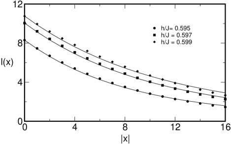
Figure 2: Comparison between $\langle l(x)\rangle_{w}$ obtained in Ref. Albano by Ising model computer simulations for boundary magnetic fields $h/J=0.595$ (circles), $h/J=0.597$ (squares) and $h/J=0.599$ (diamonds); and the approximation given by Eq. (30) (continuous lines). The Ising model parameters are: $\alpha=\pi/4$, the temperature $T=T_{c}/2$ and the bulk magnetic field $H_{bulk}=0$. The boundary magnetic field at the critical filling is $h_{c}/J=0.606$. The lengths $|x|$ and $\langle l(x)\rangle_{w}$ are measured in lattice spacing units. See text for explanation.

To finish our discussion about the $1-$point distribution functions, we compare our results with computer simulations of the 2D Ising model Albano . Close to the filling transition point, we expect that the approximate solution to Eq. (28) for $n=1$ will be generalized for arbitrary $\alpha$ to:

$$\langle l(x)\rangle_{w}\approx\frac{\langle l\rangle_{\pi}}{\cos\alpha}+\left(\langle l(0)\rangle_{w}-\frac{\langle l\rangle_{\pi}}{\cos\alpha}\right)\textrm{e}^{-x/\xi_{F}}$$ (30)

where now $\xi_{F}$ is defined as $\langle l(0)\rangle_{w}/\tan\alpha$. We have tested this approximation with the simulation results reported in Ref. Albano (see Fig. 2). The symbols correspond to the simulation data obtained for an square $64\times 64$ Ising lattice with zero bulk magnetic field and boundary magnetic fields $+h$ for the boundary rows ending at the lower left corner, and $-h$ for the remaining boundary rows. In this geometry, $\alpha=\pi/4$. The temperature is set to $T=T_{c}/2$, where $T_{c}$ is the bulk critical temperature. For this temperature and $\alpha$ the critical filling transition occurs at $h_{c}/J=0.606$. Fig. 2 shows the computer simulation results for $h/J=0.595,0.597$ and $0.599$. We have no direct estimation of $\langle l\rangle_{\pi}$. However, we have obtained $\langle l\rangle_{\pi}$ by fitting the simulation data with $|x|\leq 16$ lattice spacings (in order to minimize the effect of the upper left and lower right heterogeneous wedges) to the Eq. (30). The best fitting values are, in lattice spacing units, $\langle l\rangle_{\pi}=0.314,0.335,0.436$ for $h/J=0.595,0.597,0.599$, respectively. As it can be seen, the fitting to the simulation data is quite good, despite the crude approximations involved in Eq. (30).

Now we want to characterize the $2-$point correlations, in particular the correlations between the interfacial position above the wedge midpoint and the corresponding to an arbitrary $x$, which are given by the following function:

$$\langle(l(x)-\langle l(x)\rangle_{w})(l(0)-\langle l(0)\rangle_{w})\rangle_{w}\equiv$$

$$\langle l(x)l(0)\rangle_{w}-\langle l(x)\rangle_{w}\langle l(0)\rangle_{w}=\frac{1}{2\Sigma}\left(\frac{\partial\langle l(x)\rangle_{w}}{\partial\alpha}\right)$$ (31)

Substituting Eq. (21) into Eq. (31), we obtain:

$$\langle l(x)l(0)\rangle_{w}-\langle l(x)\rangle_{w}\langle l(0)\rangle_{w}=\sqrt{\frac{x}{2\pi\Sigma}}\frac{(2\alpha-\theta)\textrm{e}^{-\frac{\Sigma\theta^{2}}{2}x}}{2\Sigma\alpha(\theta-\alpha)}$$

$$+\frac{1}{8\Sigma^{2}\theta^{2}}\left(\frac{\theta^{2}}{(\theta-\alpha)^{2}}-\frac{\theta^{2}}{\alpha^{2}}\right)\textrm{erfc}\left(\sqrt{\frac{\Sigma\theta^{2}}{2}x}\right)$$

$$+\frac{\textrm{e}^{2\Sigma\alpha x(\alpha-\theta)}}{8\Sigma^{2}\theta}\Bigg{[}\frac{\theta}{(\theta-\alpha)^{2}}+\frac{\theta}{\alpha^{2}}$$

$$+\frac{2\Sigma(\theta-2\alpha)^{2}\theta x}{\alpha(\theta-\alpha)}\Bigg{]}\textrm{erfc}\left(\sqrt{\frac{\Sigma x}{2}}(\theta-2\alpha)\right)$$ (32)

This function decays exponentially to zero for large $x$. However, the characteristic correlation length $\xi_{x}$ (see Fig. 1) depends on $\alpha$: it is $\xi_{\parallel}$ for $\theta>2\alpha$ and $\xi_{F}$ if $\alpha<\theta<2\alpha$. Consequently, the disorder point not only introduce a new length scale for the average interfacial profile, but also for the interfacial fluctuations.

IV Results for the Kratzer binding potentials

The Kratzer binding potential (see Eq. (17)) is the marginal case between the filling mean-field and filling fluctuation regimes. For such potentials the wedge midpoint probability distribution function also obeys wedge covariance Eq. (2):

$$P_{w}^{1}(l_{0};\theta,\alpha)=\frac{[2\Sigma(\theta-\alpha)]^{2\phi+1}l_{0}^{2\phi}}{\Gamma[2\phi+1]}\exp(-2\Sigma(\theta-\alpha)l_{0})$$

$$=P_{\pi}^{1}(l_{0};\theta-\alpha)$$ (33)

It is possible to extend the transfer analysis and obtain exact results for other quantities of interest. Consider, for example, the $1-$point probability distribution function $P_{w}(l,x)$. The Laplace transform $\tilde{P}_{w}(l;E)$ can be expressed as:

$$\tilde{P}_{w}(l;E) = \int_{0}^{\infty}dl_{0}\textrm{e}^{\Sigma(2\alpha-\theta)l_{0}}\frac{(2\Sigma\theta)^{2\phi+1}(l_{0}l)^{\phi}}{\Gamma[2\phi+1]}$$ (34)

$$\times \exp(-\Sigma\theta l)\tilde{Z}_{\pi}(l_{0},l,E-\Sigma\theta^{2}/2)$$

where $\tilde{Z}_{\pi}(l_{0},l,E)$ is given by Eq. (18). This reduces to:

$$\tilde{P}_{w}(l;E)=\frac{l^{\phi}(2\Sigma\theta)^{2\phi+1}\textrm{e}^{-\Sigma\theta l}}{\theta\Gamma[2\phi+1]\Gamma[2\phi]}\kappa\Gamma\left[\phi\left(1-\kappa\right)\right]$$

$$\times\Bigg{\{}\int_{0}^{\infty}l_{0}^{\phi}\textrm{e}^{\Sigma(2\alpha-\theta)l_{0}}W_{\kappa\phi,\phi-\frac{1}{2}}\left(\frac{2\Sigma\theta l_{0}}{\kappa}\right)$$

$$M_{\kappa\phi,\phi-\frac{1}{2}}\left(\frac{2\Sigma\theta l}{\kappa}\right)-\int_{0}^{l}l_{0}^{\phi}\textrm{e}^{\Sigma(2\alpha-\theta)l_{0}}$$

$$\times\Bigg{[}W_{\kappa\phi,\phi-\frac{1}{2}}\left(\frac{2\Sigma\theta l_{0}}{\kappa}\right)M_{\kappa\phi,\phi-\frac{1}{2}}\left(\frac{2\Sigma\theta l}{\kappa}\right)$$

$$-W_{\kappa\phi,\phi-\frac{1}{2}}\left(\frac{2\Sigma\theta l}{\kappa}\right)M_{\kappa\phi,\phi-\frac{1}{2}}\left(\frac{2\Sigma\theta l_{0}}{\kappa}\right)\Bigg{]}\Bigg{\}}$$ (35)

where $\kappa\equiv 1/\sqrt{1-2E/\Sigma\theta^{2}}$. The poles of $\tilde{P}_{w}(l;E)$ in the $E$ real positive semi-axis are the characteristic inverse length scales across the wedge of $P_{w}(l,x)$. Since the second integral is over a finite interval and the integrand does not diverges in that range, no new length scale emerges from it. For the first integral, we take into account that book :

$$\int_{0}^{\infty}x^{\nu-1}\exp(-px)W_{\kappa,\mu}(ax)dx=$$

$$\frac{\Gamma[\mu+\nu+1/2]\Gamma[\nu-\mu+1/2]a^{\mu+\frac{1}{2}}}{\Gamma[\nu-\kappa+1](p+a/2)^{\mu+\nu+\frac{1}{2}}}$$

$$\times_{2}F_{1}\left(\mu+\nu+\frac{1}{2},\mu-\kappa+\frac{1}{2};\nu-\kappa+1;\frac{p-\frac{a}{2}}{p+\frac{a}{2}}\right)$$ (36)

where ${}_{2}F_{1}(a,b,c;x)$ is a hypergeometric function. If $\theta>2\alpha$, the integral does not introduce any new characteristic length . However, for $\alpha<\theta<2\alpha$ a new singularity emerges for $\Sigma(\theta-2\alpha)+\Sigma\theta/\kappa=0$, i.e. $E=2\Sigma\alpha(\theta-\alpha)=1/\xi_{F}$. Remarkably, $\xi_{F}$ has the same expression as for contact binding potentials, and is proportional (but not equal) to $\langle l(0)\rangle_{w}/\alpha$.

From this it follows that the non-thermodynamic singularity occuring at $\theta=2\alpha$ mentioned in the previous Section is not specific to contact potentials. A simple geometrical argument given in Ref. Wood explains why. The most relevant interfacial fluctuations are those where the interface leaves the substrate with a contact angle $\theta$ (relative to the tilted wall) at an arbitrary substrate point. If $\theta>2\alpha$, the other side of the wedge does not play any role and we can anticipate that the only length scale that controls the $1-$point distribution decay is $\xi_{\parallel}$. However, if $\theta<2\alpha$, the interface will eventually reach the other substrate, and consequently we can expect the geometry to play an important role leading to the emergence of a new length scale. Formally, this non-thermodynamic singularity occurs when the following integrals that arise from the spectral expansion of $Z_{\pi}(l_{1},l_{2};x)$:

$$\int_{0}^{\infty}\psi_{0}(l)\exp(2\Sigma\alpha l)\psi^{*}_{p}(l)$$ (37)

become ill-defined. There, $\psi_{p}(l)$ are the scattering eigenstates with eigenvalues $E=p^{2}/2\Sigma$ and $\psi_{0}(l)$ is the ground eigenstate. A straightforward WKB asymptotic analysis for the eigenfunctions shows that, for $p\neq 0$, the integrals given by Eq. (37) become ill-defined for $\theta<2\alpha$ for quite arbitrary choices of binding potential.

As $\theta/\alpha$ decreases, $\xi_{F}$ exceeds the intrinsic interfacial length scales $1/(E_{i}-E_{0})$, and becomes the true correlation length across the wedge $\xi_{x}$ at an another disorder point when $\xi_{F}=\xi_{\parallel}$ (recall that $\xi_{x}=\xi_{\parallel}$ for $\theta/\alpha$ larger than the value at the disorder point). For the case of contact binding potentials both non-thermodynamic singularities occur the same value $\theta=2\alpha$. However, in general, the non-thermodynamic singularities are distinct provided there are at least two bounded eigenstates of Eq. (10). For the pure Coulomb case ($\phi=1$) the second disorder point occurs at $\theta=4\alpha/3$.

Close to the new singularity $\xi_{F}^{-1}$ we found that:

$$P_{w}(l;E)\sim\frac{1}{(\xi_{F}^{-1}-E)^{1+\frac{2\phi\alpha}{2\alpha-\theta}}}\quad E\xi_{F}\to 1^{-}$$ (38)

so $P_{w}(l,x)$ behaves asymptotically for large values of $x$ as $x^{\frac{2\phi\alpha}{2\alpha-\theta}}\exp(-x/\xi_{F})$, provided that $\xi_{\parallel}<\xi_{F}$.

A field equation analogous to Eq. (25) can be found for Kratzer potentials. Transfer matrix calculations for arbitrary binding potentials lead to the relation:

$$\langle 0|\textrm{e}^{2\Sigma\alpha l}|0\rangle\Bigg{\{}\frac{\theta-\alpha}{\theta}\left[P_{w}(l,x)+\xi_{F}\left(\frac{\partial P_{w}(l,x)}{\partial x}\right)\right]$$

$$-\int_{0}^{\infty}dl_{0}\frac{\bar{\psi}_{0}^{\prime}(l_{0})}{\Sigma\theta\bar{\psi}_{0}(l_{0})}P_{w}(l_{0},0;l,x)\Bigg{\}}=L_{\pi}(l,x)$$

$$-\int_{0}^{\infty}dl_{0}\frac{\bar{\psi}_{0}^{\prime}(l_{0})}{\Sigma\theta\bar{\psi}_{0}(l_{0})}P_{\pi}(l_{0},0;l,x)$$ (39)

where $\bar{\psi}_{0}(l_{0})\equiv\psi_{0}(l_{0})\exp(\Sigma\theta l_{0})$ and $\bar{\psi}_{0}^{\prime}(l_{0})$ is its derivative respect to $l_{0}$ (recall that $\psi_{0}(l_{0})$ is the ground state eigenfunction). For Kratzer potentials, $\bar{\psi}_{0}(l_{0})\propto l_{0}^{\phi}$, so Eq. (39) can be expressed as:

$$\left(\frac{\theta}{\theta-\alpha}\right)^{\phi}\frac{\partial P_{w}(l,x)}{\partial\alpha}$$

$$+\frac{\partial}{\partial\alpha}\Bigg{[}\xi_{F}\left(\frac{\theta}{\theta-\alpha}\right)^{\phi}\frac{\partial P_{w}(l,x)}{\partial x}\Bigg{]}=0$$ (40)

As for the contact binding potential case, some interesting quantities can be evaluated from this expression. For example, the wedge adsorption is found to be:

$$\Gamma_{w}=(2\phi+1)(\phi+1)\Gamma^{CP}$$ (41)

where $\Gamma^{CP}$ is the adsorption corresponding to the contact binding potential Eq. (22).

V The breather mode picture

In order to understand the origin of the new correlation length $\xi_{F}$ we identified in previous Sections, we recall the definition of the $2-$point distribution function for $x_{2}>x_{1}\geq 0$, Eq. (13). This expression can be written in the following way:

$$P_{w}^{c}(l_{2},x_{2}|l_{1},x_{1})=P_{\pi}^{c}(l_{2},x_{2}|l_{1},x_{1})\equiv P_{\pi}^{c}(l_{2},x_{2}-x_{1}|l_{1},0)$$ (42)

where $P_{w}^{c}(l_{2},x_{2}|l_{1},x_{1})$ and $P_{\pi}^{c}(l_{2},x_{2}|l_{1},x_{1})$ are, respectively, the wedge and planar conditional probability of the interface being at a relative height $l_{2}$ from the substrate at $x_{2}$, provided that the interface is pinned at a relative height $l_{1}$ at $x_{1}$, defined as:

$$P_{i}^{c}(l_{2},x_{2}|l_{1},x_{1})=\frac{P_{i}(l_{1},x_{1};l_{2},x_{2})}{P_{i}(l_{1},x_{1})}$$ (43)

where the subscript $i$ indicates if this probability is considered in the wedge ($i=w$) or in the planar ($i=\pi$) geometry.

In view of the identity between the wedge and planar conditional probability distribution functions we first consider the of a planar substrate. The conditional probability can be obtained as:

$$P^{c}_{\pi}(l_{2},x|l_{1},0)=\frac{\psi_{0}^{*}(l_{2})}{\psi_{0}^{*}(l_{1})}\textrm{e}^{-\frac{\Sigma\theta^{2}}{2}x}Z_{\pi}(l_{1},l_{2};x)$$ (44)

For contact binding potentials, Eq. (44) can be written explicitely as:

$$P^{c}_{\pi}(l_{2},x|l_{1},0)=\sqrt{\frac{\Sigma}{2\pi x}}\textrm{e}^{-\frac{\Sigma(l_{2}-l_{1}+\theta x)^{2}}{2x}}$$

$$+\textrm{e}^{-2\Sigma\theta l_{2}}\Bigg{[}\sqrt{\frac{\Sigma}{2\pi x}}\textrm{e}^{-\frac{\Sigma(l_{1}+l_{2}-\theta x)^{2}}{2x}}$$

$$+\Sigma\theta\textrm{erfc}\left(\sqrt{\frac{\Sigma}{2\pi x}}(l_{1}+l_{2}-\theta x)\right)\Bigg{]}$$ (45)

If $l_{1}$ is very large compared with $\langle l\rangle_{\pi}\equiv 1/2\Sigma\theta$, we can identify two different behaviors of $P^{c}_{\pi}(l_{2},x|l_{1},0)$ as a function of $l_{2}$ (see Fig. 3). If $x<l_{1}/\theta$, the conditional probability is basically the free interface conditional probability that fluctuates around an average value $\langle l_{2}(x)\rangle=l_{1}-\theta x$, with a standard deviation of the order of $\sqrt{x/\Sigma}$. For $x>l_{1}/\theta$, the conditional probability becomes the $1-$point planar planar distribution function $P_{\pi}(l_{2})=2\Sigma\theta\exp(-2\Sigma\theta l_{2})$, completely uncorrelated to the value of $l_{1}$. The transition between the two regimes occur in an $x$ interval around $x_{t}=l_{1}/\theta$ which has a width of order of $\sqrt{2l_{1}/\Sigma\theta^{3}}\equiv\sqrt{x_{t}\xi_{\parallel}}$. These results are confirmed by the exact evaluation of the first moments of the conditional probability:

$$\langle l_{2}^{n}\rangle^{c}(l_{1},x)=\int_{0}^{\infty}dl_{2}\ l_{2}^{n}P^{c}_{\pi}(l_{2},x|l_{1}0)$$ (46)

The average conditional interfacial profile, which corresponds to $n=1$, is given by:

$$\langle l_{2}\rangle^{c}(l_{1},x)=(l_{1}-\theta x)+\sqrt{\frac{\Sigma}{2\pi x}}\textrm{e}^{-\frac{\Sigma(l_{1}-\theta x)^{2}}{2x}}$$

$$+\left[\frac{1}{4\Sigma\theta}-\frac{l_{1}-x\theta}{2}\right]\textrm{erfc}\left(\sqrt{\frac{\Sigma}{2\pi x}}(l_{1}-\theta x)\right)$$

$$-\frac{\textrm{e}^{2\Sigma\theta l_{1}}}{4\Sigma\theta}\textrm{erfc}\left(\sqrt{\frac{\Sigma}{2\pi x}}(l_{1}+\theta x)\right)$$ (47)

and the conditional roughness $\xi_{\perp}^{c}(l_{1},x)$ is defined as $\sqrt{\langle l_{2}^{2}\rangle^{c}-\langle(l_{2}\rangle^{c})^{2}}$, where $\langle l_{2}^{2}\rangle^{c}(l_{1},x)$ can be written as:

$$\langle l_{2}^{2}\rangle^{c}(l_{1},x)=\left[(l_{1}-\theta x)^{2}+\frac{x}{\Sigma}\right]-\Bigg{(}\frac{1}{\Sigma\theta}-l_{1}+$$

$$\theta x\Bigg{)}\sqrt{\frac{\Sigma}{2\pi x}}\textrm{e}^{-\frac{\Sigma(l_{1}-\theta x)^{2}}{2x}}+\Bigg{[}\frac{x}{2\Sigma}-\frac{1}{4\Sigma^{2}\theta^{2}}+$$

$$\frac{(l_{1}-x\theta)^{2}}{2}\Bigg{]}\textrm{erfc}\left(\sqrt{\frac{\Sigma}{2\pi x}}(l_{1}-\theta x)\right)$$

$$+\left[x\theta+l_{1}-\frac{1}{2\Sigma\theta}\right]\frac{\textrm{e}^{2\Sigma\theta l_{1}}}{2\Sigma\theta}\textrm{erfc}\left(\sqrt{\frac{\Sigma}{2\pi x}}(l_{1}+\theta x)\right)$$ (48)

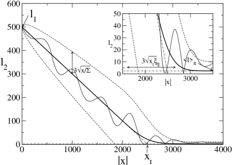
Figure 3: Illustration of a typical interfacial configuration pinned at $l_{1}\gg\langle l\rangle_{\pi}$ for $x=0$ (thin continuous line). We have set $\Sigma=1$ (it defines the length scale), $\theta=0.2$ and $l_{1}=500$. The thick continuous line corresponds to the conditional average profile $\langle l_{2}\rangle^{c}(l_{1},x)$, and the dotted lines correspond to $\max(0,\langle l_{2}\rangle^{c}(l_{1},x)\pm 3\xi_{\perp}^{c}(l_{1},x))$ where $\xi_{\perp}^{c}(l_{1},x)$ is the conditional roughness. Any interfacial configuration has a probability of at least 95% of being between the dotted lines. Inset: an enlargement of the area around $x_{t}=l_{1}/\theta$. Other characteristic length scales are represented. See text for explanation.

We obtain two main conclusions from these results when $l_{1}\gg\langle l\rangle_{\pi}$. First, the interfacial positions are highly correlated to the the central one for $|x|<l_{1}/\theta$. Secondly, the intrinsic interfacial fluctuations are small in this $x$ range compared to the conditional average value. Actually, if we set $l_{1}$ as the length scale, the rescaled conditional probability distribution function $\tilde{P}_{\pi}^{c}(l_{2}/l_{1},x/l_{1}|1,0)\equiv l_{1}P_{\pi}^{c}(l_{2},x|l_{1},0)$ behaves as:

$$\tilde{P}_{\pi}^{c}(l_{2}/l_{1},x/l_{1}|1,0)\to\delta\left(\frac{l_{2}-l_{1}+\theta x}{l_{1}}\right)H(l_{1}-\theta x)$$

$$+\delta\left(\frac{l_{2}}{l_{1}}\right)H(\theta x-l_{1})$$ (49)

when $\Sigma\theta l_{1}\to\infty$. We expect this result to be valid for any potential and also for random bond disorder, since in all these cases the wandering exponent for the free interface $\zeta<1$. this can be checked for the marginal $1/l$ potential. The Laplace transform of the conditional probability distribution as:

$${\cal L}\left[P_{\pi}^{c}(l_{2},x|l_{1},0)\right]\equiv\int_{0}^{\infty}dx\ \textrm{e}^{Ex}P_{\pi}^{c}(l_{2},x|l_{1},0)$$

$$=\frac{\psi_{0}^{*}(l_{2})}{\psi_{0}^{*}(l_{1})}\tilde{Z}_{\pi}(l_{1},l_{2},E-\Sigma\theta^{2}/2)$$ (50)

For $\Sigma\to\infty$ at fixed $E,\theta,l_{1}$ and $l_{2}$ , and taking into account Eq. (18) and that the ground state eigenfunction $\psi_{0}(l)\propto l^{\phi}\exp(-\Sigma\theta l)$, we obtain the following behavior for the Laplace transform of the conditional probability distribution function:

$${\cal L}\left[P_{\pi}^{c}(l_{2},x|l_{1},0)\right]\to\frac{1}{\theta}H(l_{1}-l_{2})\textrm{e}^{E(l_{1}-l_{2})/\theta}-\frac{\delta(l_{2})}{E}\textrm{e}^{El_{1}/\theta}$$ (51)

The Laplace transform can be inverted, leading to Eq. (49).

To proceed, we return to our discussion about the wedge geometry. Due to the presence of the boost factor $\exp(2\Sigma\alpha l)$ in the midpoint probability distribution function, the midpoint interfacial height is almost always further from the substrate than the mean wetting layer thickness $\langle l\rangle_{\pi}$ for any binding potential. If we assume that the conditional probability distribution function is given by Eq. (49), which corresponds to as neglecting the intrinsic interfacial fluctuations around the conditional interfacial profile, we can capture the main features of both the average interfacial profile and the correlations along the wedge for contact binding potentials. Actually, this picture is completely equivalent to the 2D wedge breather mode model Parry4 ; Parry2 .

The average interfacial profile can be written as:

$$\langle l(x)\rangle_{w}=\int_{0}^{\infty}dl_{1}P_{w}(l_{1},0)\left[\int_{0}^{\infty}dl_{2}l_{2}P_{\pi}^{c}(l_{2},x|l_{1},0)\right]$$

$$\approx\int_{\theta x}^{\infty}dl_{1}P_{w}(l_{1},0)(l_{1}-\theta x)=\int_{0}^{\infty}sP_{w}(s+\theta x,0)ds$$ (52)

The behavior of $\langle l(x)\rangle_{w}$ for large $x$ is dominated by the large $l$ asymptotics of $P_{w}(l,0)$. The latter can be obtained by taking into account Eq. (14) for $m=n=0$ and making use of the WKB approximation for the $1-$point planar distribution function:

$$P_{\pi}(l)\sim\frac{1}{\sqrt{1+\frac{2W(l)}{\Sigma\theta^{2}}}}\exp\left(-2\Sigma\theta\int^{l}dt\sqrt{1+\frac{2W(t)}{\Sigma\theta^{2}}}\right)$$

$$\sim\textrm{e}^{-2\Sigma\theta l}\exp\left(-2\int^{l}dt\frac{W(t)}{\theta}\right)\quad l\to\infty$$ (53)

The first thing we can see is that, for large $x$, the decay of $\langle l(x)\rangle_{w}$ in this approximation is controlled by an exponential term $\exp[-2\Sigma\theta(\theta-\alpha)x]$. So, a new length scale $\xi_{F}^{*}$ is defined as $1/2\Sigma\theta(\theta-\alpha)$. Close to the filling transition, $\xi_{F}^{*}=\xi_{F}-1/2\Sigma\alpha\theta\sim\xi_{F}+{\cal O}(1)$.

Depending on the large $l$ behavior of the (attractive) binding potentials, different situations can arise Parry3 . The filling mean field regime is characterized by binding potentials that decay to zero as $1/l^{p}$ where $p<1/\zeta-1$, implying $\zeta<1$ for thermal disorder (the wandering exponent $\zeta=1/2$). A saddle point calculation shows that close to the filling transition $\langle l(0)\rangle_{w}\sim 1/\Sigma(\theta-\alpha)^{p}$. As $\theta\to\alpha$, the relevant length scale in the $x$ direction, $\langle l(0)\rangle_{w}/\theta\gg\xi_{F}^{*}$, so the latter length scale is irrelevant (in fact, intrinsic interfacial fluctuations that we neglected can be more important).

For $p=1$, both length scales become of the same order, and consequently $\langle l(x)\rangle_{w}\sim\langle l(0)\rangle_{w}f(x/\xi_{F}^{*})\exp(-x/\xi_{F}^{*})$, where $f(x)$ diverges at most algebraically, and depends on the detailed structure of the binding potential through the short distance $l$ dependence of $P_{w}(l,0)$. For a pure $1/l$ potential, $f(x)=(1+2x/3+x^{2}/6)$. This expression verifies the differential equation for $\langle l(x)\rangle_{w}$ that arises from Eq. (40) in the scaling limit.

The filling fluctuation regime corresponds to potentials with $p>1$, and is characterized by universal critical exponents and scaling functions. Indeed in the critical regime the scaling behavior is the same as that found for contact binding potentials. For $x\to\infty$, we find that asymptotically $\langle l(x)\rangle_{w}\sim\langle l(0)\rangle_{w}\exp(-x/\xi_{F}^{*})$. This solution agrees with the asymptotics of $\langle l(x)\rangle_{w}$ for contact binding potentials when $\theta\to\alpha$, although with a decay length slightly smaller. However, the behaviour is asymptotically correct if we assume that $\xi_{F}^{*}\equiv\xi_{F}$.

For the correlation functions, we have:

$$\langle l(x)l(0)\rangle_{w}-\langle l(x)\rangle_{w}\langle l(0)\rangle_{w}=\int_{0}^{\infty}dl_{1}l_{1}P_{w}(l_{1},0)\Delta(l_{1},x)$$ (54)

where $\Delta(l_{1},x)$ is defined as:

$$\Delta(l_{1},x)=\int_{0}^{\infty}dl_{2}l_{2}\left[P_{\pi}^{c}(l_{2},x|l_{1},0)-P_{w}(l_{2},x)\right]$$ (55)

In the breather mode approximation, $\Delta(l_{1},x)$ can be obtained as:

$$\Delta(l_{1},x)\approx(l_{1}-\theta x)H(l_{1}-\theta x)-\langle l(x)\rangle_{w}$$ (56)

We find different behaviors depending on the value of $p$. In the filling mean field regime, $\Delta(l_{1},x)$ is negligible in this scale. For the filling fluctuation regime, the correlation function decays as:

$$\langle l(x)l(0)\rangle_{w}-\langle l(x)\rangle_{w}\langle l(0)\rangle_{w}\sim\langle l(0)\rangle_{w}^{2}\left(1+\frac{x}{\xi_{F}^{*}}\right)\textrm{e}^{-\frac{x}{\xi_{F}^{*}}}$$ (57)

and again is in agreement with the behavior of the exact correlation function for contact binding potentials Eq. (32) when $x\to\infty$ and $\theta\to\alpha$ (assuming again that $\xi_{F}^{*}\equiv\xi_{F}$). Finally, for the marginal case $p=1$ the behavior of the correlation function is predicted to be for $x\to\infty$ as $\langle l(0)\rangle_{w}^{2}g(x/\xi_{F}^{*})\exp(-x/\xi_{F}^{*})$, where $g(x)$ is a function that diverges at most algebraically.

Another quantity of interest is the midpoint local susceptibility $\chi_{w}(l)$, defined as:

$$\chi_{w}(l)=\frac{\partial\rho(l)}{\partial h}\Bigg{|}_{h=0}=2(\rho_{l}-\rho_{v})\int_{l}^{\infty}dsP_{w}(s,0)\bar{\Delta}(s)$$ (58)

where $\bar{\Delta}(l)\equiv\int_{0}^{\infty}dx\Delta(l,x)$. In the breather mode approximation and in the filling fluctuation regime, $\bar{\Delta}(s)$ has the following expression:

$$\bar{\Delta}(l)=\frac{1}{\theta}\left(\frac{l^{2}}{2}-\langle l(0)\rangle_{w}^{2}\right)$$ (59)

which is exact for contact binding potentials. This expression, together with the midpoint wedge covariance Eq. (2), leads to the covariance relationship between the local susceptibilities Parry3 :

$$\chi_{w}(l;\theta,\alpha)=\frac{\theta-\alpha}{\theta}\chi_{\pi}(l,\theta-\alpha)$$ (60)

where $\chi_{\pi}(l,\theta)$ is the local susceptibility corresponding to the planar geometry for a contact angle $\theta$.

Finally, we note that the breather mode picture has direct consequences for the scaling of the interfacial profile in the filling fluctuation regime. To see this, recall that the wedge midpoint probability distribution function scales as Parry3 :

$$P_{w}(l)=\frac{1}{\langle l(0)\rangle_{w}}\Lambda\left(\frac{l}{\langle l(0)\rangle_{w}}\right)$$ (61)

where $\Lambda(s)$ is a universal function and, due to covariance, is the same as the scaling function for the corresponding planar $1-$point probability distribution function. Complementing the scaling of the probability distribution function is the position dependence of the interfacial profile, which we anticipate satisfies:

$$\langle l(x)\rangle_{w}=\langle l(0)\rangle_{w}\phi\left(\frac{\theta x}{\langle l(0)\rangle_{w}}\right)$$ (62)

where $\phi(s)$ is another universal function. In the breather mode picture, the interface is infinitely stiff in the filled region implying that the scaling functions $\Lambda(s)$ and $\phi(s)$ are related via:

$$\phi(s)=\int_{s}^{\infty}d\bar{s}\Lambda(\bar{s})(\bar{s}-s)$$ (63)

or equivalently:

$$\phi^{\prime\prime}(s)=\Lambda(s)$$ (64)

A remarkable consequence of this relation is that the behavior of the interfacial profile close to the midpoint is determined by the short distance behavior of the wedge midpoint $1-$point probability distribution function. Since $\Lambda(s)\sim s^{\frac{1}{\zeta}-2}$ as $s\to 0$ Parry3 , we have $\phi(s)\sim 1-|s|+A|s|^{\frac{1}{\zeta}}$ for small $s$. Note that the first two terms are needed to preserve the continuity of the true interfacial profile $\langle y(x)\rangle_{w}$ and its derivative at the wedge midpoint. This result suggests that the interface behaves, for small values of $x$, as a random walk of $x$ as a function of $z$. This prediction is consistent with the behaviour of $\langle l(x)\rangle_{w}$ for contact binding potentials in the scaling limit $\theta\to\alpha$, $\xi_{\parallel}/\xi_{F}\to 0$ but $x/\xi_{F}$ finite.

Finally, note that Eq. (64) is also obeyed by the (non-universal) scaling functions corresponding to the marginal case.

VI Renormalization group approach to the critical filling transition

In this Section we will justify the critical properties of the filling transition using a renormalization group framework. Specifically we will generalize an exact decimation functional renormalization group procedure previously used to study 2D critical wetting Huse ; Lipowsky ; Spohn . Our transfer matrix results show that geometry plays a fundamental role in determining the critical behavior, so we anticipate that the appropiate renormalization group procedure must preserve the wedge shape. This implies that the effective wandering exponent $\zeta$ determining the rescaling of the interfacial height $l$ must be $\zeta=1$. This contrasts with the value $\zeta=1/2$, which is appropiate for free interfaces and also planar wetting transtions. We will see that this choice leads naturally to the breather mode picture of the filling transition, implying that interfacial fluctuations are irrelevant except for those that determine the wedge midpoint interfacial position.

Before introducing the renormalization group scheme, we generalize some of the results of previous Sections. The set of $(2n+1)-$point distribution functions that includes the midpoint interfacial position can be obtained in terms of the planar case counterpart by Eq. (14). If we set $\theta=\alpha$, it is clear from that expression that $P_{w}(-n;\ldots;n)\equiv 0$ at the critical filling transition for any value of $n$. However, all the correlation functions decay at the same rate, since Eq. (14) can be rewritten as:

$$P_{w}(-n;\ldots;n)=P_{w}(0)\frac{P_{\pi}(-n;\ldots;n)}{P_{\pi}(0)}$$ (65)

Consequently, the conditional $(2n+1)-$point probability distribution function remains finite at the filling transition. The only relevant operator (in a renormalization group sense) should be related only to the $1-$point probability distribution function at the midpoint. Taking into account Eq. (11) and the definition of the $2-$point conditional probability distribution function Eq. (44), we can rewrite Eq. (65) as

$$P_{w}(-n;\ldots;n) = P_{w}(0)\prod_{i=0}^{n-1}P_{\pi}^{c}(l_{i+1},x_{i+1}-x_{i}|l_{i},0)$$ (66)

$$\times \prod_{i=-n}^{-1}P_{\pi}^{c}(l_{i},x_{i+1}-x_{i}|l_{i+1},0)$$

where we have chosen the ground state eigenfunction to be real and positive. The $2-$point conditional probability distribution function has a non-trivial limit when $\Sigma\theta l_{1}\to\infty$ (see Eq. (49)). Our goal will be to find a renormalization group scheme in which the $2-$point conditional probability distribution function converges to this limit, and the only relevant operator is related to the wedge midpoint $1-$point distribution function.

Let us consider a discrete version of the interfacial hamiltonian Eq. (3):

$$\beta H=\sum_{i=-n}^{n-1}\left\{\frac{\Sigma}{2}(z_{i+1}-z_{i})^{2}+W(z_{i}-i\alpha)\right\}$$ (67)

where the spacing between sites $a=1$ defines the length unit for $l$, $\Sigma^{-1}$, etc. Using a similar transformation to the continuous case, Eq. (67) can be written as:

$$\beta H[l]=2n\frac{\Sigma\alpha^{2}}{2}+2\Sigma\alpha l_{n}-2\Sigma\alpha l_{0}$$

$$+\sum_{i=-n}^{n-1}\left\{\frac{\Sigma}{2}(l_{i+1}-l_{i})^{2}+\frac{W(l_{i})+W(l_{i+1})}{2}\right\}$$ (68)

where periodic boundary conditions have been applied ($l_{n}=l_{-n}$). To simplify our discussion, we will consider $n\to\infty$ and neglect the boundary effects. The probability of any interfacial configuration is given by:

$$P_{w}(\{l_{i}\})=\frac{\textrm{e}^{-\beta H}}{Z}=\textrm{e}^{2\Sigma\alpha l_{0}+\beta f_{W}}\prod_{i=-\infty}^{\infty}\textrm{e}^{-\beta{\cal\tilde{H}}(l_{i},l_{i+1})}$$ (69)

where ${\cal\tilde{H}}(l_{i},l_{i+1})$ is defined as:

$$\beta{\cal\tilde{H}}(l_{i},l_{i+1})=\beta f_{s}+\frac{\Sigma}{2}(l_{i+1}-l_{i})^{2}+\frac{W(l_{i})+W(l_{i+1})}{2}$$ (70)

where $f_{s}$ is the planar surface free energy per unit length and is related to the contact angle corresponding to the binding potential $W(l)$ via:

$$\beta f_{s}=\frac{1}{2}\ln\left(\frac{\Sigma}{2\pi}\right)-\frac{\Sigma\theta^{2}}{2}$$ (71)

For $\theta=0$, $\beta f_{s}$ converges towards the free interface free energy per unit length. Note that in the continuum limit Eq. (6), this term is absorbed in the path measure. On the other hand, $\beta f_{W}$ is defined as:

$$\beta f_{W}=\lim_{n\to\infty}\left\{\left(-{\ln Z}+2n\frac{\Sigma\alpha^{2}}{2}\right)-2n\beta f_{s}\right\}$$ (72)

that corresponds to the wedge excess free energy (we suppose that this quantity is well-defined). Note that ${\cal\tilde{H}}(l_{i},l_{i+1})$ is invariant under an exchange of its arguments.

Let us now consider a decimation procedure, similar to the one used for the study of 2D critical wetting. We group the sites in blocks of $b$ units, keeping the first one and integrating over all the interfacial positions of the remaining $b-1$ sites in the block. Since the site $i=0$ plays a special role, the sites to be kept in each decimation step are those with $i=jb$, with $j\in\mathbb{Z}$. After that, we rescale $x$ positions by a factor $b$ and $l$ by a factor $b^{\zeta}$, i.e.:

$$x\to x^{\prime}=\frac{x}{b}\quad;\quad l_{i}\to l_{j}^{\prime}=\frac{l_{jb}}{b^{\zeta}}$$ (73)

The new hamiltonian $\beta{\cal\tilde{H}^{\prime}}(l_{j}^{\prime},l_{j+1}^{\prime})$ is defined as:

$$\textrm{e}^{-\beta{\cal\tilde{H}^{\prime}}(l_{j}^{\prime},l_{j+1}^{\prime})}=b^{\zeta}\int_{0}^{\infty}dl_{1}\textrm{e}^{-\beta{\cal\tilde{H}}(b^{\zeta}l_{j}^{\prime},l_{1})}$$

$$\ldots\int_{0}^{\infty}dl_{b-1}\textrm{e}^{-\beta{\cal\tilde{H}}(l_{b-1},b^{\zeta}l_{j+1}^{\prime})}$$ (74)

Note that the renormalized hamiltonian $\beta{\cal\tilde{H}}^{\prime}(l_{1},l_{2})$ is symmetrical under an exchange of its arguments provided that the original $\beta{\cal\tilde{H}}(l_{1},l_{2})$ is also symmetrical (even if it is not defined as Eq. (70)). This procedure is iterated, leading to a sequence of renormalized hamiltonians.

In order to complete the description of the renormalization group (RG) procedure we should give the transformation rules for $\alpha$ and $\beta f_{W}$. First we revisit the planar geometry ($\alpha=f_{W}=0$). We will consider the value of the exponent $\zeta$ arbitrary, unlike in Refs. Huse ; Lipowsky ; Spohn , where $\zeta=1/2$. In general, after an arbitrary number of RG steps, we can write any $\beta{\cal\tilde{H}}(l_{i},l_{i+1})$ as:

$$\beta{\cal\tilde{H}}(l_{i},l_{i+1})=\frac{\Sigma}{2}(l_{i+1}-l_{i})^{2}+\tilde{W}(l_{i},l_{i+1})$$

$$+\frac{1}{2}\ln\left(\frac{\Sigma}{2\pi}\right)-\frac{\Sigma\theta^{2}}{2}$$ (75)

where $\tilde{W}(l_{i},l_{i+1})$ is a symmetric function under exchange of its arguments. Obviously, in principle this function need not decay to zero when both arguments are large (as it does in Eq. (70)). However let us suppose that it decays as $-A/[(l_{i}+l_{i+1})/2]^{p}$ when $l_{i},l_{i+1}\to\infty$. After making a RG step, we would like to find the asymptotic behavior of the renormalized $\tilde{W}^{\prime}(l_{j}^{\prime},l_{j+1}^{\prime})$ for large enough $l_{j}^{\prime}$, $l_{j+1}^{\prime}$. Expanding the RHS of Eq. (74) and keeping terms up to first order in $W$ (since $l_{j}^{\prime}$ and $l_{j+1}^{\prime}$ are large, the values of $l_{1}\ldots l_{b-1}$ that contribute most to the integral are also very large), we find that:

$$\textrm{e}^{-\beta{\cal\tilde{H}^{\prime}}}\approx b^{\zeta}\textrm{e}^{b\frac{\Sigma\theta^{2}}{2}}\int_{0}^{\infty}dl_{1}\sqrt{\frac{\Sigma}{2\pi}}\exp\left(-\frac{\Sigma(b^{\zeta}l_{j}^{\prime}-l_{1})^{2}}{2}\right)$$

$$\ldots\int_{0}^{\infty}dl_{b-1}\sqrt{\frac{\Sigma}{2\pi}}\exp\left(-\frac{\Sigma(l_{b-1}-b^{\zeta}l_{j+1}^{\prime})^{2}}{2}\right)$$

$$\times\Bigg{[}1-W(b^{\zeta}l_{j}^{\prime},l_{1})-W(l_{b-1},b^{\zeta}l_{j+1}^{\prime})$$

$$-\sum_{i=1}^{b-2}W(l_{i},l_{i+1})\Bigg{]}$$ (76)

The lowest order term (corresponding to set $W=0$) can be estimated for large $l_{j}^{\prime},l_{1},\ldots,l_{b-1},l_{j+1}^{\prime}$ by extending the lower integration limits to $-\infty$, and has the value:

$$b^{\zeta}\textrm{e}^{b\frac{\Sigma\theta^{2}}{2}}\int_{-\infty}^{\infty}dl_{1}\sqrt{\frac{\Sigma}{2\pi}}\exp\left(-\frac{\Sigma(b^{\zeta}l_{j}^{\prime}-l_{1})^{2}}{2}\right)$$

$$\ldots\int_{-\infty}^{\infty}dl_{b-1}\sqrt{\frac{\Sigma}{2\pi}}\exp\left(-\frac{\Sigma(l_{b-1}-b^{\zeta}l_{j+1}^{\prime})^{2}}{2}\right)$$

$$=\textrm{e}^{b\frac{\Sigma\theta^{2}}{2}}\sqrt{\frac{\Sigma b^{2\zeta-1}}{2\pi}}\exp\left(-\frac{\Sigma b^{2\zeta-1}(l_{j}^{\prime}-l_{j+1}^{\prime})^{2}}{2}\right)$$ (77)

So, in order that the renormalized binding potential $W^{\prime}$ decays to zero at large values of both its arguments, the interfacial stiffness and the contact angle must transform as:

$$\Sigma\to\Sigma^{\prime}=\Sigma b^{2\zeta-1}\quad;\quad\theta\to\theta^{\prime}=\theta b^{1-\zeta}$$ (78)

Two comments are pertinent at this point. Firstly, the transformation of the interfacial stiffness is also valid for a free interface. Secondly, the change in the contact angle has a geometrical interpretation, since its scaling Eq. (78) corresponds exactly to the change of small angles under the coordinates scaling Eq. (73). Thus it is reasonable to expect that $\alpha$ must change in the same way.

If we take into account the first order in $W$, we can characterize the decay of the renormalized potential at large values of $l_{j}^{\prime}$ and $l_{j+1}^{\prime}$. For simplicity, we consider the case $b=2$. The renormalized binding potential has the following expression:

$$W^{\prime}(l_{j}^{\prime},l_{j+1}^{\prime})\approx\sqrt{\frac{\Sigma}{\pi}}\int_{-\infty}^{0}dl_{1}\textrm{e}^{-\Sigma\left(l_{1}-2^{\zeta}\frac{l_{j}+l_{j+1}}{2}\right)^{2}}$$

$$+\sqrt{\frac{\Sigma}{\pi}}\int_{0}^{\infty}dl_{1}\textrm{e}^{-\Sigma\left(l_{1}-2^{\zeta}\frac{l_{j}+l_{j+1}}{2}\right)^{2}}\Bigg{[}W(2^{\zeta}l_{j}^{\prime},l_{1})$$

$$+W(l_{1},2^{\zeta}l_{j+1}^{\prime})\Bigg{]}=W^{\prime}_{1}(l_{j}^{\prime},l_{j+1}^{\prime})+W^{\prime}_{2}(l_{j}^{\prime},l_{j+1}^{\prime})$$ (79)

The first term $W_{1}^{\prime}$ corresponds to the contribution of the hard wall to the renormalized binding potential, and $W_{2}^{\prime}$ corresponds to the contribution of the original binding potential $W$. The hard wall contribution can be evaluated exactly as:

$$W^{\prime}_{1}(l_{j}^{\prime},l_{j+1}^{\prime})=\frac{1}{2}\textrm{erfc }\left[\sqrt{\frac{2^{2\zeta}\Sigma}{\pi}}\left(\frac{l_{j}^{\prime}+l_{j+1}^{\prime}}{2}\right)\right]$$

$$\approx\frac{\exp\left[-\frac{2^{2\zeta}\Sigma}{\pi}\left(\frac{l_{j}^{\prime}+l_{j+1}^{\prime}}{2}\right)^{2}\right]}{\sqrt{2^{2\zeta}\Sigma}(l_{j}^{\prime}+l_{j+1}^{\prime})}\quad l_{j}^{\prime}+l_{j+1}^{\prime}\to\infty$$ (80)

For $W_{2}^{\prime}$, we take into account the long distance behavior of $W$. After some algebra, the leading order of $W_{2}^{\prime}(l_{j}^{\prime},l_{j+1}^{\prime})$ can be written as:

$$W_{2}^{\prime}(l_{j}^{\prime},l_{j+1}^{\prime})\approx-\frac{2^{1-\zeta p}A}{(\bar{l}_{j}^{\prime})^{p}}\int_{-s_{0}/2}^{\infty}ds\frac{\textrm{e}^{-s^{2}}/\sqrt{\pi}}{\left[1+s/s_{0}\right]^{p}}$$ (81)

where $\bar{l}_{j}^{\prime}\equiv(l_{j}^{\prime}+l_{j+1}^{\prime})/2$ and $s_{0}\equiv\sqrt{\pi}2^{\zeta+1}\bar{l}_{j}^{\prime}$. As $\bar{l}_{j}^{\prime}\to\infty$, the integral tends to 1 and we can see that $W^{\prime}\sim W^{\prime}_{2}\sim A^{\prime}/(\bar{l}_{j}^{\prime})^{p}$, where $A^{\prime}=Ab^{1-\zeta p}$. It is interesting to note that this result is also obtained by the following scaling argument for the binding potential:

$$\frac{A}{l^{p}}\to\frac{A^{\prime}}{(l^{\prime})^{p}}=b\frac{A}{l^{p}}=b\frac{A}{(b^{\zeta}l^{\prime})^{p}}=\frac{Ab^{1-\zeta p}}{(l^{\prime})^{p}}$$ (82)

where we have taken into account that the binding potential is a free energy per $x$ unit length.

This analysis shows that the RG procedure leaves invariant the functional dependence of the asymptotic behavior of the binding potential. Two regimes can be identified. If $p>1/\zeta$, the binding potential strength decreases in each RG step. For $p<1/\zeta$ the binding potential strength grows in each RG step. Finally, the marginal case $p=1/\zeta$ corresponds to the leading asymptotic behavior remaining invariant. For $\zeta=1/2$, which is the relevant value for planar wetting phenomena, this behavior leads to the existence of two and three fluctuation regimes for complete and critical wetting, respectively Fisher . Note that this choice of $\zeta$ keeps the relevant microscopic scale $\xi_{b}\sim\Sigma^{-1}$ invariant. The analysis of the critical wetting from this RG approach can be found in Refs. Huse ; Lipowsky ; Spohn .

A special class of effective hamiltonians are the following:

$$\exp[-\beta{\cal\tilde{H}}(l_{i},l_{i+1})]=Z_{\pi}^{\Sigma,W}[l_{i},l_{i+1};1]\textrm{e}^{-\frac{\Sigma\theta^{2}}{2}}$$ (83)

where $Z_{\pi}^{\Sigma,W}[l_{i},l_{i+1};1]$ is the partition function Eq. (6) with $x=a\equiv 1$ for arbitrary values of the interfacial stiffness and binding potential $W(l)$. Such Hamiltonians can be regarded as those which are generated after one iteration of the renormalization group provided that $b$ very large. Indeed the fixed points found in Refs. Huse ; Lipowsky ; Spohn belong to this class. Taking into account the properties of the path integrals, the renormalized potential after a RG step Eq. (74) can be written as:

$$\exp[-\beta{\cal\tilde{H}^{\prime}}(l_{j}^{\prime},l_{j+1}^{\prime})]=b^{\zeta}Z_{\pi}^{\Sigma,W}[b^{\zeta}l_{j}^{\prime},b^{\zeta}l_{j+1}^{\prime};b]\textrm{e}^{-\frac{b\Sigma\theta^{2}}{2}}$$ (84)

For contact binding potentials Eq. (6) and Kratzer potentials Eq. (18), it can be checked that Eq. (84) corresponds to an effective hamiltonian of the same form as the original since:

$$b^{\zeta}Z_{\pi}^{\Sigma,W}[b^{\zeta}l_{j}^{\prime},b^{\zeta}l_{j+1}^{\prime};b]=Z_{\pi}^{\Sigma^{\prime},W^{\prime}}[l_{j}^{\prime},l_{j+1}^{\prime};1]$$ (85)

where $\Sigma$ and $\theta$ are transformed via Eq. (78) to $\Sigma^{\prime}$ and $\theta^{\prime}$. For Kratzer potentials $w$ must change as $\Sigma^{-1}$, i.e. $w^{\prime}=wb^{1-2\zeta}=w/b$ in order to preserve the invariance of the leading order behavior under renormalization.

Finally to finish our discussion of the RG for planar critical wetting phenomena, we note that the $1-$point distribution function renormalizes as:

$$P_{\pi}^{\prime}(l_{0}^{\prime})=b^{\zeta}P_{\pi}(b^{\zeta}l_{0}^{\prime})$$ (86)

We will require this result later. Returning to our discussion about the RG in the wedge geometry, we need to provide the transformation rules for $\alpha$ and $\beta f_{W}$. We will assume that $\alpha$ changes as $\theta$:

$$\alpha\to\alpha^{\prime}=\alpha b^{1-\zeta}$$ (87)

In order to obtain the transformation rule for $\beta f_{W}$, we consider how the $1-$point midpoint wedge probability distribution function renormalizes:

$$P_{w}^{\prime}(l_{0}^{\prime},0)\equiv P_{\pi}^{\prime}(l_{0}^{\prime})\textrm{e}^{2\Sigma^{\prime}\alpha^{\prime}l_{0}^{\prime}+(\beta f_{w})^{\prime}}$$

$$=b^{\zeta}P_{\pi}(b^{\zeta}l_{0}^{\prime})\textrm{e}^{2\Sigma\alpha b^{\zeta}l_{0}^{\prime}+(\beta f_{w})^{\prime}}=b^{\zeta}P_{w}(b^{\zeta}l_{0}^{\prime},0)$$ (88)

implying that $\beta f_{w}$ remains invariant:

$$\beta f_{w}\to(\beta f_{w})^{\prime}=\beta f_{w}$$ (89)

Finally, we note that if we change the effective hamiltonian by:

$${\beta\cal H}(l_{i},l_{i+1})={\beta\cal\tilde{H}}(l_{i},l_{i+1})\pm[f(l_{i+1})-f(l_{i})]$$ (90)

where the sign is positive for $i\geq 0$ and negative for $i<0$, the probability of an interfacial configuration is now:

$$P_{w}(\{l_{i}\})=\textrm{e}^{2\Sigma\alpha l_{0}+2f(l_{0})+\beta f_{W}}\prod_{i=-\infty}^{\infty}\textrm{e}^{-\beta{\cal H}(l_{i},l_{i+1})}$$ (91)

The renormalization of the hamiltonian Eq. (74) is valid provided:

$$f^{\prime}(l_{i}^{\prime})=f(b^{\zeta}l_{i}^{\prime})+C^{\prime}$$ (92)

Note that any function $f(l_{i})$ (unless it is a constant) breaks the invariance of ${\beta\cal H}$ under exchange of its arguments and consequently introduces a directionality in the $x$ axis. This is perfectly sensible in the wedge geometry, but is not admissible for the planar substrate, where $-x$ is completely equivalent to $x$. A convenient choice for $f(l_{i})$ is:

$$f(l_{i})=\frac{1}{2}\ln P_{\pi}(l_{i})$$ (93)

where $P_{\pi}(l_{i})$ is the $1-$point probability distribution function in the planar geometry, and the condition Eq. (93) is verified due to Eq. (86). It is not difficult to see that $\exp(-{\beta\cal H})$ is the $2-$point conditional probability distribution function. Taking into account this fact and Eq. (88), it is clear that Eq. (91) is exactly the same as Eq. (66).

The one remaining issue to be decided is the relevant value of the exponent $\zeta$. We choose $\zeta=1$, so that the wedge tilt angle $\alpha$ and contact angle $\theta$ remain invariant in each step of the RG.

The procedure is now standard. The RG flow trajectories are constrained to the $\theta-$constant hypersurfaces in functional space. Since we know that the filling transition occurs for $\theta=\alpha$, we first check that this situation corresponds to the critical manifold. Instead of considering an arbitrary potential, we choose as initial effective hamiltonians those of the form given by Eq. (83), in particular with the partition function corresponding to contact binding potentials and those of Kratzer form. When the number of RG steps $n\to\infty$, the probability distribution of an interfacial configuration converges to a fixed point of the form:

$$P_{w}^{*}(\{l_{i}\})\propto l_{0}^{2\phi}\textrm{e}^{(\beta f_{W})^{*}}\prod_{i=-\infty}^{\infty}\textrm{e}^{-{\beta\cal H^{*}}(l_{i},l_{i+1})}$$ (94)

where $(\beta f_{W})^{*}=-\infty$, and $\beta\cal H^{*}$ is defined as:

$$\textrm{e}^{-{\beta\cal H^{*}}(l_{i},l_{i+1})}=\begin{cases}\delta(l_{i+1}-l_{i}+\alpha)H(l_{i}-\alpha)\\ +\delta(l_{i})H(\alpha-l_{i})&i\geq 0\\ \\ \delta(l_{i}-l_{i+1}+\alpha)H(l_{i+1}-\alpha)\\ +\delta(l_{i+1})H(\alpha-l_{i+1})&i<0\end{cases}$$ (95)

It is straightforward to see that Eq. (95) is a fixed point of Eq. (74). Obviously, since $(\beta f_{W})^{*}=-\infty$, the probability distribution for any interfacial configuration is zero. Nevertheless, we will consider Eq. (94) as formally different from zero. The basin of attraction for the $\phi=0$ case is expected to be those hamiltonians with binding potentials that decay faster than $1/l$ (corresponding to the filling fluctuation regime). Hamiltonians that have a binding potential with a leading order $-\phi\alpha/l$ will be attracted to the fixed point Eq. (94) with the same value of $\phi$ for $\theta=\alpha$ (marginal case). Finally, if $lW(l)$ diverges as $l\to\infty$, there is no fixed point and the filling transition is mean-field-like.

If $\theta\neq\alpha$, no matter how small $|\theta-\alpha|$ is, the RG flow drives the hamiltonian away from the critical manifold. For $\theta>0$, $\exp(-{\beta\cal H})$ converges to a fixed point expression Eq. (95) with $\alpha$ replaced by $\theta$. Even though this new fixed point for the conditional probability is different from the the critical fixed point, the flow for the $2-$point conditional probability distribution function will remain close (in some functional sense) to the critical one if $|\theta-\alpha|\ll\alpha$. Consequently, there is no relevant field associated with ${\beta\cal H}$.

On the other hand, the wedge midpoint $1-$point probability distribution function behaves differently. We considered the same initial effective hamiltonians as for the $\theta=\alpha$ case. If $\theta<\alpha$, the distribution has an unphysical exponential growth with $l_{0}$ as $\exp(\Sigma|\theta-\alpha|l_{0})$. The exponential term grows in each RG step, driving the probability distribution function to infinity (however, $\beta f_{w}=-\infty$, so the “real” probability of any interfacial configuration is zero). The attractor at infinity can be regarded as the complete filling fixed point. For $\theta>\alpha$, the wedge midpoint $1-$point probability distribution function becomes more and more peaked around zero as $\Sigma\to\infty$, converging to the low temperature fixed point:

$$P_{w}^{LT}(\{l_{i}\})=\prod_{i=-\infty}^{\infty}\delta(l_{i})$$ (96)

These results imply that there is a relevant field (in the RG sense) associated with $P_{w}(l_{0},0)$. Actually, the only other relevant operator is $h\propto\mu_{c}-\mu$, where $\mu$ is the chemical potential and $\mu_{c}$ the value at gas-liquid coexistence.

Recall that the critical exponents defined at coexistence ($\mu=\mu_{c}$):

$$\langle l(0)\rangle_{w}\sim t^{-\beta_{w}}\quad;\quad\xi_{\perp}(0)\sim t^{-\nu_{\perp}}$$

$$\xi_{x}\sim t^{-\nu_{x}}\quad;\quad\beta f_{W}\sim t^{2-\alpha_{w}}$$ (97)

where $t=T_{f}-T$ and $T_{f}$ is the critical filling temperature. Close to a critical filling fixed point (for any $\phi$), all the relevant scale lengths $\Sigma^{-1}$, $\langle l(0)\rangle_{w}$, $\xi_{x}$, $\xi_{\perp}(0)$, etc. are reduced by a factor $1/b$. To extract the dependence on $t$ we need to know the largest eigenvalue of the linearized RG flow close to the critical fixed point. We argued above that this eigenvalue is associated to the transformation of the $x=0$ term of the hamiltonian ${\beta\cal H}_{0}$. We again considered the special hamiltonians Eq. (83) for contact and Kratzer binding potentials. The expression of ${\beta\cal H}_{0}$ for these potentials is:

$${\beta\cal H}_{0}=2\Sigma(\theta-\alpha)l_{0}-2\phi\ln l_{0}+C$$ (98)

Taking into account how ${\beta\cal H}_{0}$ renormalizes, and its expression at the critical fixed point (see Eq. (94)), it is clear that the largest eigenvalue is $b$, and its associated eigenfunction is proportional to $\Sigma(\theta-\alpha)l_{0}$. As a consequence, the critical exponents $\nu_{\perp}=\nu_{x}=\beta_{w}=1$ for both the filling fluctuation and marginal regimes.

To get the leading singularity for the wedge excess free energy is more complicated. As $\beta f_{w}$ remains invariant under the RG transformations, $2-\alpha_{w}=0$. However, this value does not rule out a logarithmic divergence in $T_{w}-T$. In order to get such a dependence, we use the following thermodynamic relationship:

$$\left(\frac{\partial(\beta f_{w})}{\partial\alpha}\right)_{\Sigma,\theta}=-2\Sigma\langle l(0)\rangle_{w}$$ (99)

where the derivative is made without changing $\Sigma$ or any characteristic of the binding potential (in particular the contact angle). We can rewrite Eq. (99) as:

$$\left(\frac{\partial(\beta f_{w})}{\partial\Sigma(\theta-\alpha)}\right)_{\Sigma,\theta}=2\langle l(0)\rangle_{w}$$ (100)

After a renormalization step, we know that, even when $\Sigma$ and the binding potential have changed, this derivative changes as $1/b$ since $\beta f_{w}$, $\theta$ and $\alpha$ are invariant, and $\Sigma^{-1}$ and $\langle l(0)\rangle_{w}$ decrease by a factor $1/b$. If we regard $\Sigma(\theta-\alpha)$ ($\propto\Sigma$, and recall that $\theta-\alpha$ is invariant under a RG step) as proportional to $t$ when the flow is close to the critical fixed point, Eq. (100) implies that $\beta f_{w}$ diverges logarithmically as $T\to T_{f}$. Furthermore, $\beta f_{w}$ is invariant under renormalization and must vanish as $\alpha\to 0$. Consequently close to the filling transition it must be proportional dependence to $\ln(\theta-\alpha)-\ln(\theta)$.

The critical exponents obtained for the critical filling transition are in complete agreement with exact calculations and scaling arguments Parry3 .

VII Conclusions

The structure of the gas-liquid interface bound at a 2D wedge and close to the filling transition has been studied using exact transfer-matrix methods. These calculations show the emergence of a new correlation length $\xi_{F}$ sufficiently close to the phase boundary ($\alpha<\theta<2\alpha$). The explicit transfer matrix results for correlation functions and interfacial roughness completely support the breather mode picture of fluctuation effects. The same picture also emerges of a renormalization group approach that leaves the wedge geometry invariant. The fact that the only relevant fluctuations are those that translate the midpoint interfacial height leads to a simple relationship between the interfacial structure and midpoint height probability distribution function in the scaling limit. The extension of this approach to higher dimensions and/or different geometries would be very interesting and further work is being carried out in that direction.

Finally it would be instructive to understand the physical origin of the covariance relationship Eq. (2). In the filling fluctuation regime we found that covariance can be inferred from the existence of the differential relation Eq. (25) and some regularity conditions. The very existence of such a field equation is itself indicative that some unknown symmetry relates wetting and filling transitions. Further work is required to elucidate whether any such hidden symmetry exists.

References

(1) K. Rejmer, S. Dietrich and M. Napiorkowski, Phys. Rev. E
60, 4027 (1999).
(2) A. O. Parry, C. Rascón and A. J. Wood, Phys. Rev. Lett.
83, 5535 (1999).
(3) A. O. Parry, C. Rascón and A. J. Wood, Phys. Rev. Lett.
85, 345 (2000).
(4) A. O. Parry, A. J. Wood and C. Rascón, J. Phys.: Condens.
Matter 13, 4591 (2001).
(5) A. O. Parry, M. J. Greenall and A. J. Wood, J. Phys.: Condens.
Matter 14, 1169 (2002).
(6) P. Concus and R. Finn, Proc. Natl. Acad. Sci. USA 63,
292 (1969).
(7) Y. Pomeau, J. Colloid Interface Sci. 113, 5 (1986).
(8) E. H. Hauge, Phys. Rev. A 46, 4994 (1992).
(9) D. B. Abraham, A. O. Parry and A. J. Wood, Europhys.
Lett. 60, 106 (2002).
(10) D. B. Abraham and A. Maciolek, Phys. Rev. Lett. 89,
286101 (2002).
(11) E. V. Albano, A. De Virgiliis, M. Müller and K. Binder,
J. Phys.: Condens. Matter 15, 333 (2003).
(12) A. J. Wood and A. O. Parry, J. Phys. A: Math. Gen. 34, L5
(2001).
(13) T. W. Burkhardt, Phys. Rev. B 40, 6987 (1989) and
references therein.
(14) C. Grosche and F. Steiner, Handbook of Feynman
Path Integrals (Springer, Berlin, 1998).
(15) M. J. Greenall, A. O. Parry and J. M. Romero-Enrique,
in preparation.
(16)Tables of integral transforms, vol. 1, edited
by A. Erdélyi (McGraw-Hill, New York, 1954).
(17) D. A. Huse, Phys. Rev. Lett. 58, 176 (1987).
(18) F. Jülicher, R. Lipowsky and H. Müller-Krumbhaar,
Europhys. Lett. 11, 657 (1990).
(19) H. Spohn, Europhys. Lett. 14, 689 (1991).
(20) R. Lipowsky and M. E. Fisher, Phys. Rev. B 36,
2126 (1987).