Solution of a statistical mechanics model for pulse formation in lasers

Abstract

We present a rigorous statistical-mechanics theory of nonlinear many mode laser systems. An important example is the passively mode-locked laser that promotes pulse operation when a saturable absorber is placed in the cavity. It was shown by Gordon and Fischer ourPRL that pulse formation is a first-order phase transition of spontaneous ordering of modes in an effective “thermodynamic” system, in which intracavity noise level is the effective temperature. In this paper we present a rigorous solution of a model of passive mode locking. We show that the thermodynamics depends on a single parameter, and calculate exactly the mode-locking point. We find the phase diagram and calculate statistical quantities, including the dependence of the intracavity power on the gain saturation function, and finite size corrections near the transition point. We show that the thermodynamics is independent of the gain saturation mechanism and that it is correctly reproduced by a mean field calculation. The outcome is a new solvable statistical mechanics system with an unstable self-interaction accompanied by a natural global power constraint, and an exact description of an important many mode laser system.

I Introduction

Lasers can produce light in continuous wave (cw) or pulsed manners. A special pulsed operation is mode-locking, found shortly after the laser discovery in the early 1960’s PML . Since then, mode-locked lasers became a leading way to produce ultra short pulses reaching today a few femtoseconds, or about two light-wave cycles. In a mode-locked operation, many axial modes in a broad frequency bandwidth are phase locked and thus provide one or multiple pulses in the cavity, giving at the output a light pulse train. The understanding of the conditions under which a laser operates in pulsed regime rather than in continuous wave regime is a question of great interest, both theoretical and practical. This question has been addressed in various studies, being referred to as “the second threshold” (the first one being the lasing itself) in the earlier years Haken ; haken_threshold1 ; new , and recently, in the context of laser with a saturable absorber, as the “self starting” problem Krausz ; threshold2 ; threshold3 ; HausConfirm ; KrauszAnswer ; KrauszConfirm ; threshold4 ; MEstability .

Formation of pulses in lasers relies on the interaction between axial modes. Such an interaction can be provided either by rendering the system time dependent (modulating) or by a suitable nonlinearity in the dynamics of the system. These two methods are commonly referred to as “active” and “passive” mode-locking, respectively. One type of nonlinearity known to encourage pulsed operation is saturable absorption. The light transmissivity through a (fast) saturable absorber is an increasing function of the (instantaneous) input intensity. The saturable absorber destabilizes the laser operation into configurations where most of the power is concentrated in short pulses. In the frequency or mode domain the saturable absorber induces a nonlinear four-wave-mixing interaction between the modes, as does the Kerr effect, with the difference that it is dissipative rather than dispersive.

The dynamics of a laser is always subject to noise. Beside the usual noise sources present in every physical system, there is the inevitable fundamental noise of spontaneous emission. This noise is inherent in lasers, since it always accompanies coherent amplification, on which lasers rely. Therefore a model of a laser that does not take noise properly into account risks missing key features in the physics of a laser system.

The majority of laser theories treat noise as a perturbation, if at all, expecting it to manifest itself as fluctuations in the laser output. However, this approach greatly underestimates the effect of noise. It has been recently shown ourOL that even very weak noise (compared to the intracavity power of the laser) is sufficient, for example, to destabilize a passively mode-locked laser, revealing a dramatic nonperturbative effect of the noise.

We have recently developed ourPRL ; GFOC a new approach for the many interacting mode system, with specific emphasis on aspects of pulse formation in mode-locked lasers. We established an analogy between the behavior of the electromagnetic field (the mode system in a laser) in the presence of noise and equilibrium statistical mechanics, and applied the powerful tools of statistical mechanics to the problem of mode-locking. In particular it was found that the entropy associated with the noise is an essential ingredient in the theory of mode locking. This approach gave an inherent explanation for many experimental phenomena of mode-locked lasers, especially the existence of a threshold and the abruptness of formation of pulses. Passive mode locking was identified with a first-order phase transition in the model statistical mechanics system. Many other theoretical and experimental features CLEO were found, among them, hysteresis, super-heating and super-cooling, successive formation of multiple pulses in the cavity and more.

The results of Ref. ourPRL were based on a mean field analysis of the mode interaction induced by the saturable absorber and on numerical simulations. These indicated a first order phase transition when the effective temperature, i.e. the noise power, or alternatively the intracavity power, is varied. The ordered phase corresponds to a mode locked configuration, while the disordered phase to continuous wave operation.

In this paper we show that the statistical-mechanics treatment of mode locking suggested in ourPRL can be concluded with an exact solution. Using a recursion relation for the partition function, we are able to develop a systematic expansion of the free energy in decreasing powers of the number of degrees of freedom. The first two terms in this expansion are calculated explicitly, allowing us to show that there is indeed a single first order phase transition associated with passive mode locking. All the relevant thermodynamic quantities are obtained, yielding a complete description of mode locking in the context of the present model. We also present an improved mean field analysis, which turns out to be exact in the thermodynamic limit.

We show that the thermodynamics depends on a single parameter, the strength of the saturable absorption multiplied by the intracavity power squared, and divided by the noise strength, and the transition occurs when this parameter crosses an explicit threshold value.

In addition, we demonstrate the universality of the results with respect to the gain saturation mechanism (as long as it is slow). It is well known that gain saturation, that is, the inability of the laser amplifier to amplify the light indefinitely, has a crucial role in understanding the dynamics and stability of lasers Siegman and in particular mode-locked lasers MenyukPMLstability . While in Ref. ourPRL gain saturation was incorporated by introducing a constraint of strictly constant intracavity power, in this paper we present a solution with general (slow) gain saturation mechanism. The relation between the two approaches is similar to that of the canonical and grand-canonical ensembles in textbook statistical mechanics, and the saturable gain acts in manner analogous to the chemical potential. The universality property follows immediately from the thermodynamic equivalence of ensembles. Futhermore, for a given gain saturation function we are able to calculate the dependence of the intracavity power on the external parameters, and in particular its jump at the mode-locking transition, an experimentally-measurable quantity.

As a statistical mechanics problem, the model can be likened to a gas of (complex) spins, with a $|\psi|^{4}$ self interaction, and a global constraint of total amplitude, quite similar to the constraint imposed on spins in the Berlin-Kac spherical model berlin-kac . Normally the statistical mechanics of such systems leads to simple equipartition. Here, however, the energy of self interaction term is negative, and at small enough temperature, or high enough power the instability stemming from the self-interaction drives the system into a pulsed state, where most of the power resides in a single spin. In Fourier (mode or wavenumber $k$) representation the model is equivalent to a classical complex spin chain with a special nonlocal interaction that drives the mode locking transition, which in this representation is a standard ordering transition. Fig. 1 shows the difference between typical mode-locked and non-mode-locked configurations in Fourier space, and in real space in the context of the coarse grained model discussed below.

                                   

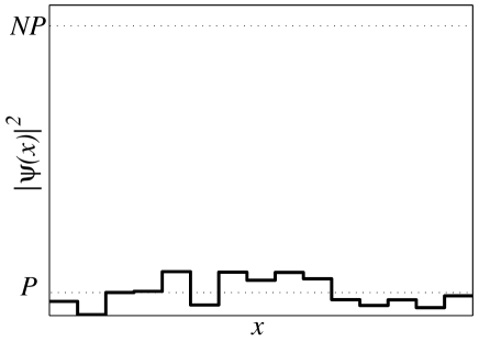
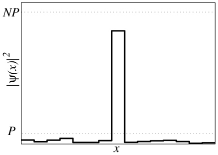
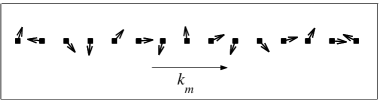
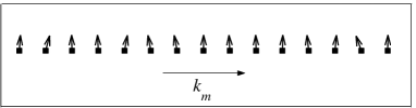
Figure 1: The two “thermodynamic phases”: A typical non-mode-locked configuration is shown on the left column of the figure and a mode-locked one on the right. The real space configurations of the coarse grained model are shown on top row, see Eqs. (17,18) for definitions. The Fourier modes $a_{m}$, defined in Eq. (22) at discrete wavenumbers $k_{m}$, are displayed on the bottom row as a set of phasors, each arrow representing the complex value of a Fourier mode.

While in this work the quartic self-interaction is attributed to saturable absorption, the model can be put into a broader context. The quartic interaction is of general interest being the lowest-order nonlinearity which is translation, inversion and rotation invariant and local. This interaction itself has been very extensively studied, but we are not aware of previous statistical-mechanics studies of its interplay with a non-local power constraint. In some previous well-known statistical-mechanics studies of lasers Haken , this non-local constraint did not exist in the model, which may explain why the mode-locking noise-induced threshold behavior has not been previously found. Since a global limitation of power is common in physical systems, our model may be an important prototype in nonlinear optics and elsewhere.

II Models of passive mode locking

II.1 The coarse-graining approximation

The propagation of the wave packet in a laser cavity is a non-equilibrium process: A stationary condition is characterized by constant pumping and dissipation of energy. Noise, due to spontaneous emission is also present. The temporal evolution of the wavepacket envelope $\psi$ is given schematically by

$$\partial_{t}\psi(x,t)=G[\psi](x,t)+\eta(x,t)\ ,$$ (1)

where $G$ is the net gain, and $\eta$ is a random driving. $\psi$ is defined on the interval $0\leq x\leq L$ with periodic boundary conditions.

In the context of passive mode-locking, the net gain functional has three essential components: $G=G_{\hbox{\scriptsize gain}}+G_{\hbox{\scriptsize sa}}+G_{\hbox{\scriptsize sp}}$. The net pumping of energy by stimulated emission is modelled by

$$G_{\hbox{\scriptsize gain}}(x,t)=g\!\!\left({\mathcal{P}}\right)\psi(x,t)\ ,$$ (2)

where ${\mathcal{P}}=\frac{1}{L}\int_{0}^{L}|\psi(x,t)|^{2}\,dx$ is the total power in the cavity. The saturable gain function $g$ is monotonically decreasing with positive values for small ${\mathcal{P}}$ and negative for large ${\mathcal{P}}$ where various losses overcome the power supplied by the amplifier.

A necessary ingredient for passive mode locking is saturable absorption, wherein the dissipation losses decrease as the power increases. Unlike the saturable amplifier, the response of the saturable absorber is fast, so it depends on the instantaneous power $|\psi|^{2}$ rather than on the total power ${\mathcal{P}}$. We choose the specific form of saturable absorption

$$G_{\hbox{\scriptsize sa}}(x,t)=\gamma_{s}|\psi(x,t)|^{2}\psi(x,t)\ ,$$ (3)

with $\gamma_{s}>0$, valid for $|\psi|^{2}$ not too large HausReview . Note that since losses are already taken into account in $G_{\hbox{\scriptsize gain}}$, the saturable absorption term describes an additional “gain” term which is absent when $\psi=0$.

The third part models the spectral dependence of the amplifier that has a characteristic frequency, which we assume lies at the center of the wavepacket. Define the Fourier expansion of the wavepacket

$$\psi(x,t)=\sum_{m=-\infty}^{\infty}b_{m}(t)e^{\frac{2\pi imx}{L}}\ .$$ (4)

Near the resonance, the pumping efficiency falls down quadratically in the spectral distance. The net gain for modes off the center of the band is therefore reduced by

$$G_{\hbox{\scriptsize sp}}(m,t)=-\gamma_{g}\Big{(}\frac{2\pi m}{L}\Big{)}^{2}b_{m}(t)\ ,$$ (5)

where $\gamma_{g}$ is positive.

The resulting gain functional can be expressed as the functional derivative $G(x,t)=-\delta\mathsf{H}[\psi]/\delta\psi^{*}(x)$ of

$${\mathsf{H}}[\psi] = \int_{0}^{L}dx\,(-\frac{\gamma_{s}}{2}|\psi(x)|^{4}+\gamma_{g}|\psi^{\prime}(x)|^{2})$$ (6)

$$+ LU\!\Big{(}\frac{1}{L}\int_{0}^{L}|\psi(x,t)|^{2}\,dx\Big{)}\ ,$$ (7)

with the definition $U^{\prime}({\mathcal{P}})=-g({\mathcal{P}})$.

The random part $\eta$ of Eq. (1) will be modelled by (complex) gaussian uncorrelated noise with a power of $2LT$

$${\left<\eta^{*}(x,t)\eta(x^{\prime},t^{\prime})\right>}=2TL\delta(x-x^{\prime})\delta(t-t^{\prime}),$$

${\left<\cdot\right>}$ stands for an ensemble average. This is appropriate for spontaneous emission. We arrive thus at the explicit equation of motion for $\psi$

$$\partial_{t}\psi(x,t)=-\frac{\delta{\mathsf{H}}[\psi]}{\delta\psi^{*}(x)}+\eta(x,t)\ ,$$ (8)

It is well known ourPRL ; risken that the invariant measure of gradient flow with additive white noise, such as Eq. (8) is

$$\rho[\psi]=\mathsf{Z}^{-1}e^{-{\mathsf{H}}[\psi]/(LT)}\ ,$$ (9)

where the partition function is

$$\mathsf{Z}=\int[d\psi][d\psi^{*}]e^{-{\mathsf{H}}[\psi]/(LT)}\ .$$ (10)

The study of passive mode locking in our model has been reduced to the analysis the statistical mechanics system described by $\mathsf{Z}$.

The model which is summarized by Eqs. (6,10) does not include refractive effects such as dispersion and the Kerr nonlinearity (imaginary terms), which are important in most laser systems. Nevertheless, as pointed out in a previous work GFOC , $\rho$ serves as the invariant measure when dispersive effects are included, provided that a certain integrability condition holds. Ref. GFOC also studied in some detail the consequences of the failure of the integrability condition to hold. The purpose of the present work is different: By simplifying the model even further, we obtain a system which captures all the essential qualitative features of the passive mode locking transition in a transparent and intuitive manner.

The spectral filtering term $\gamma_{g}|\psi^{\prime}(x)|^{2}$ in $\mathsf{H}$ introduces correlations between the electric field in neighboring positions. It counteracts the tendency of the saturable absorption to concentrate the power in a thinner and thinner interval by introducing a length scale over which the electric field is correlated. This suggests a coarse graining approximation, in which the electric field is assumed to be constant on an interval, and the interaction between adjacent intervals is neglected. The function $\psi$ is then represented on the interval by a single degree of freedom (see Fig. 1).

Taking $N$ such intervals we find that

$$\tilde{H}_{N}[\psi]=-\frac{\gamma_{s}L}{2N}\sum_{n=1}^{N}|\psi_{n}|^{4}-LU\!\!\left({\mathcal{P}}\right)$$ (11)

where now

$${\mathcal{P}}=\frac{1}{N}\sum_{n}|\psi_{n}|^{2}$$ (12)

and

$$\tilde{Z}_{N}=\int\prod_{n}\frac{d\psi_{n}d\psi^{*}_{n}}{2\pi}\,e^{{-\tilde{H}_{N}}[\psi]/(LT)}\ .$$ (13)

The statistical mechanics problem defined by Eqs. (11-13) is the main object of study in this paper. At zero temperature, which corresponds to noiseless dynamics, the quartic term in $\tilde{H}$ pushes all the available power into a single degree of freedom (whose identity depends on the initial conditions). This is the mode-locked state. In the opposite situation at high $T$ or $\gamma_{s}=0$ the power is randomly distributed, and mode-locking is absent.

II.2 The thermodynamic limit

Our analysis relies crucially on $N$ being very large. In the way we stated the problem, $N$ is the ratio between the laser cavity length and the width of a pulse. In short-pulse laser this parameter is large by definition, with values anywhere in the interval $10^{2}$–$10^{9}$. Taking $N\to\infty$ and expanding in $1/N$ looks therefore promising.

It is not difficult to see, however, that the statistical mechanics system in Eqs. (11-13) has no well defined thermodynamic-limit behavior as $N\to\infty$. For example, the $T=0$ value of the intracavity power ${\mathcal{P}}$ is the minimum of

$$-\frac{1}{2}\gamma_{s}NL{\mathcal{P}}^{2}-LU({\mathcal{P}})$$ (14)

with respect to ${\mathcal{P}}$, which diverges with $N$. As usual in such cases, this means that we should “renormalize” the parameters of the Hamiltonian, i.e. let $\gamma_{s}$, $T$ and the function $U$ depend on $N$ in such a way that a well-defined thermodynamic limit is obtained. A comparison with a concrete example or experiment requires a preliminary translation of the renormalized parameters to the actual parameters.

However, a more fundamental difficulty remains: Due to the nature of the mode-locking transition, the ratio of the peak power, the maximal value of $|\psi_{n}|^{2}$, to the intracavity power diverges like $N$ when $N$ is large. This means that only one of these quantities can achieve a well-defined thermodynamic limit, while the other quantity has to be rescaled. For example one can choose parameters such that the peak power and $N{\mathcal{P}}$ achieve finite thermodynamic limiting values. This is convenient when a more general form of saturable absorber is assumed HausReview .

In the present paper (as well as in Ref. ourPRL ), because the nonlinearity is a homogeneous function (of degree 4) it is more convenient to choose parameters such that the total power ${\mathcal{P}}$ reaches a well defined limit $P$, and the peak power diverges linearly in $N$. When this is used in Eq. (11) the quartic term is seen to scale linearly in $N$. We choose the saturable gain function such that it scales in the same way,

$$U_{N}({\mathcal{P}})\equiv NTu({\mathcal{P}})$$ (15)

for some fixed function $u$ ($T$ is added to the definition for later convenience). In this scheme $T$ and $\gamma_{s}$ need not be renormalized.

Since the mode-locked configuration is characterized by peak power proportional to $N$, a natural order parameter is

$$M=\Big{(}\frac{1}{N^{2}}\sum_{n}{\left<|\psi_{n}|^{4}\right>}\Big{)}^{1/4}\ ,$$ (16)

where ${\left<\right>}$ stands for expectation with respect to the invariant measure. The peak power in the non-mode-locked case is $O(1)$ in the thermodynamic limit, so $M=0$ there.

II.3 Fixed power ensemble

Since the quartic term in the Hamiltonian $\tilde{H}$ is unbounded from below, the gain saturation term $U({\mathcal{P}})$ is essential to ensure stability, preventing the system from cascading into states with arbitrarily low $\tilde{H}$. This reflects the well known fact that lasers owe their stability to gain saturation Siegman ; MenyukPMLstability . This is analogous to the role of the chemical potential in the grand-canonical ensemble in standard statistical mechanics, which limits the number of particles in the system.

An alternative approach is to suppose that the intracavity power ${\mathcal{P}}$ has a fixed value $P$, whose analogue in textbook statistical mechanics is the canonical ensemble where the number of particles is fixed. This is the scheme used in Ref. ourPRL . One of the main results of the present work is an equivalence of ensembles. The thermodynamics obtained in the fixed- and variable-power ensembles are equivalent. The variable-power ensemble has to be used if ${\left<{\mathcal{P}}\right>}$ is not known. These issues are discussed in sec. V.

In the fixed power ensemble there is no need to include the gain saturation term, and the partition function is defined by

$$Z_{N}(\gamma_{s},T,P)=\int\prod_{n}\frac{d\psi_{n}d\psi^{*}_{n}}{2\pi}\,e^{\frac{-H_{N}[\psi]}{T}}\delta({\mathcal{P}}[\psi]-P)\ ,$$ (17)

with the reduced Hamiltonian

$$H_{N}[\psi]=-\frac{\gamma_{s}}{2N}\sum_{n=1}^{N}|\psi_{n}|^{4}\ .$$ (18)

The change of variables $y_{n}=|\psi_{n}|^{2}$ in Eq. (17) leads to the simpler form

$$Z_{N}(\gamma_{s},T,P)=\int\prod_{n}dy_{n}\,e^{\frac{\gamma_{s}}{2NT}\sum_{n}y_{n}^{2}}\delta\left(\frac{1}{N}\sum_{n=1}^{N}\!y_{n}-P\right)\ ,$$ (19)

where the $y_{n}$ integrations are from $0$ to $\infty$. Another change of variables $y_{n}\to Py_{n}$ leads to the useful scaling relation

$$Z_{N}(\gamma_{s},T,P)=P^{N-1}{\mathcal{Z}}_{N}(\gamma_{s}P^{2}/T)$$ (20)

where

$${\mathcal{Z}}_{N}(\gamma)\equiv Z_{N}(\gamma,1,1)\ .$$

An important conclusion has already been reached: The thermodynamics depends on the single parameter $\gamma\equiv\gamma_{s}P^{2}/T$. Eq. (20) proves this in the fixed power scheme, while the equivalence of ensembles extends this to the general case.

In Sec. IV we solve the statistical mechanics problem in the fixed-power ensemble by developing an asymptotic expansion for ${\mathcal{Z}}_{N}$ for large $N$, which is valid and uniform for all $\gamma$.

III Mean field theory

The problem lends itself to a mean field analysis when formulated in Fourier (mode) space. In the Fourier representation mode-locking manifests as ordering in the phases of the various modes, see Fig 1. The discrete Fourier transform of the Hamiltonian (18) is

$$H[a]=-\frac{\gamma_{s}}{2}\sum_{m_{1}-m_{2}+m_{3}-m_{4}=pN}a_{m_{1}}^{*}a_{m_{2}}a_{m_{3}}^{*}a_{m_{4}}$$ (21)

where

$$\psi_{n}=\sum_{m=1}^{N}a_{m}e^{2\pi im\frac{n}{N}}$$ (22)

and $p$ is an integer (actually it is easy to see that only $p=-1,0,1$ are relevant). ${\mathcal{P}}$ is now given by

$${\mathcal{P}}=\sum_{m}|a_{m}|^{2}.$$ (23)

The main disadvantage of the Fourier space formulation is that the nonlinear term becomes complicated and nonlocal. Mean field theory overcomes this difficulty by assuming that the different modes are uncorrelated and characterized by a common probability distribution function $\rho_{\hbox{\scriptsize mf}}(a)$. When the problem is formulated in Fourier space, the mean field approximation is quite plausible, since the interaction term involves all the degrees of freedom.

In the mean field framework the free energy per degree of freedom is

$$F\equiv-\frac{\log Z}{N}=-\frac{\gamma_{s}}{2T}N^{2}|{\left<a\right>}_{\hbox{\scriptsize mf}}|^{4}+{\left<\log\rho\right>}_{\hbox{\scriptsize mf}}\ ,$$ (24)

where ${\left<\right>}_{\hbox{\scriptsize mf}}$ stands for expectation value with respect to $\rho_{\hbox{\scriptsize mf}}$. Gain saturation is included by demanding that

$${\left<|a|^{2}\right>}_{\hbox{\scriptsize mf}}=\frac{P}{N}\ ,$$ (25)

i.e. ${\left<{\mathcal{P}}\right>}_{\hbox{\scriptsize mf}}=P$.

Following the standard procedure of mean field calculations zinn-justin , $\rho_{\hbox{\scriptsize mf}}$ is found by minimizing the free energy subject to the constraint Eq.(25). A necessary condition for the minimization of $F$ is stationarity with respect to variations of $\rho$,

$$0 = \frac{\delta}{\delta\rho(a)}\left(F+\lambda\left({\left<|a|^{2}\right>}-P/N\right)\right)=$$

$$= -2\mathop{\rm Re}(\gamma_{s}/T)N^{2}|{\left<a\right>}|^{2}{\left<a^{*}\right>}a+(\log\rho(a)+1)+\lambda|a|^{2},$$

where $\lambda$ is a Lagrange multiplier. The solution of Eq. (III) is a gaussian probability distribution function

$$\rho(a)=\frac{1}{\pi\sigma^{2}}e^{-\frac{|a-{\left<a\right>}|^{2}}{\sigma^{2}}}\ .$$ (27)

${\left<a\right>}$ and $\sigma$ are related by Eq. (25) which implies

$${\left<|a|^{2}\right>}_{\hbox{\scriptsize mf}}=|{\left<a\right>}_{\hbox{\scriptsize mf}}|^{2}+\sigma^{2}=\frac{P}{N}\ .$$ (28)

$\rho_{\hbox{\scriptsize mf}}$ is therefore characterized by the single parameter $M=\sqrt{N/P}|{\left<a\right>}_{\hbox{\scriptsize mf}}|$. From Eq. (28) one can see that $0\leq|M|^{2}\leq 1$. When $M=0$ the phases of the modes are completely random, which means that in real space the power is uniformly distributed. When $M>0$ the modes are correlated which in real space means that a macroscopic fraction of the power resides in the variable $\psi_{N}$. $M$ is therefore an order parameter, which can be shown to asymptotically coincide with the previous definition of the order parameter Eq. (16).

We note that the present formulation of mean field theory is slightly careless, in that it misses ordered states centered at other points than $\psi_{N}$ in real space. The inclusion of these configurations would require considering cases where various $a_{m}$’s differ by a fixed phase. However, since the number of missed configurations grows only linearly with $N$, the entropy is underestimated by a subextensive factor, and the thermodynamics is not affected.

We can define a new thermodynamic potential $f(\gamma,y)$, where $y=M^{2}$ and $\gamma=\gamma_{s}P^{2}/T$, which is the free energy for a given value $M$. Using Eqs. (27-28) in Eq. (24) it is found that

$$f(\gamma,y)=-\left(\frac{\gamma}{2}y^{2}+\log(1-y)\right)\ ,$$ (29)

up to unimportant additive terms independent of $\gamma$ and $M$. The free energy $F$ for given $\gamma$ is the global minimum of $f(\gamma,\cdot)$, and the abscissa of the minimum, $\bar{y}$, is the square of the order parameter.

The function $f$ of Eq. (29) has a single minimum for $\gamma\leq 4$, at $y_{0}=0$. The vanishing of $M$ means that the phases are not locked corresponding to the disordered, non mode-locked phase. For $\gamma>4$ there exists an additional (local) minimum, $y_{1}>0$, see Fig. 2, which corresponds to the mode-locked state. However, for $4\leq\gamma\leq\gamma^{*}\simeq 4.91$ $f(\gamma,y_{1})>f(\gamma,y_{0})$, which means that the mode-locked state is metastable, and the true equilibrium is still disordered, $\bar{y}=y_{0}$. At $\gamma=\gamma^{*}$ the two minima exchange stability, and for all $\gamma>\gamma^{*}$ the equilibrium state is mode locked, with $\sqrt{y_{1}}$ as the value of the order parameter. $\gamma^{*}$ is the solution of the equation $f(\gamma,y_{0})=f(\gamma,y_{1}(\gamma))$,

$$\frac{{\left({{\sqrt{\gamma^{*}}+\sqrt{\gamma^{*}-4}}}\right)}^{2}}{8}=\log\frac{\sqrt{\gamma^{*}}(\sqrt{\gamma^{*}}+\sqrt{\gamma^{*}-4})}{2}$$ (30)

Figure 2: The thermodynamic potential $f(\gamma,y)$ as a function of $y=M^{2}$ for several values of $\gamma$ ranging from 2 to 6 with higher values of $\gamma$ corresponding to lower curves. Curves with two (local) minima correspond to systems with a metastable state. The critical $\gamma$ ($\gamma^{*}$) is by definition the one where the values of $f(\gamma,\cdot)$ at the two minima are equal, which implies a first order phase transition.

In terms of the original variables $\gamma_{s}$, $T$ and $P$, the phase transition point is therefore

$$\frac{\gamma_{s}P^{2}}{T}=\gamma^{*}\approx 4.91$$ (31)

In order to compare it to the result in Ref. ourPRL , one should remember the difference in the modeling of spectral filtering here and there. In Ref. ourPRL we imposed “Dirichlet” boundary conditions in the Fourier space, while here, the coarse graining method actually induces periodic boundary consitions in Fourier space. Since the interaction in Fourier space is long ranged, this leads to a difference. The Hamiltonian in Ref. ourPRL was identical to Eq. (21), except that $p=0$ only. The number of quartets with $k=0$ is 2/3 of their number with $p=-1,0,1$. In the mean field approximation this would simply lead to a factor of $3/2$ in the transition temperature:

$$\frac{\gamma_{s}P^{2}}{T}=\frac{3}{2}\gamma^{*}\approx 7.4$$ (32)

This is very close to the result of $\gamma_{s}P^{2}/T\approx 7.7$ obtained in Ref. ourPRL . (We note that the mode locking transition was specified in Ref. ourPRL in terms of $1/\gamma$.) The mean field theory presented here is better, since here we do not make the ansatz of separating the modulus and angle in $\rho_{\rm mf}$. Here we also end up with the simple analytical expression (29). Since the Hamiltonian (21) is translation invariant in Fourier space, mean field theory is more suitable for its analysis than for that of its counterpart from Ref. ourPRL .

In summary, it has been demonstrated in the mean field context that the mode locking transition is a standard first order transition, accompanied by coexistence and metastable configurations in its neighborhood. The mean field theory involves an uncontrolled approximation, which is hard to justify rigorously. In the present work the justification will ultimately follow from the real space analysis given in the next section.

Evidently, the transition condition depends, although not greatly, on the spectral filtering scheme. Analysis of the parabolic filtering scheme, which we do not pursue here, yields a yet another value for the transition temperature, close to (31) and (32).

IV Fixed power finite $N$ analysis

In this section we calculate an asymptotic expansion of the partition function $Z_{N}(\gamma,P)$ in decreasing powers of $N$, the number of degrees of freedom. All information pertaining to the passive mode-locking transition is then obtainable in a standard manner. In particular, we show that the mean field calculations give the exact free energy.

Our starting point is a recursive version of Eq. (19) for $Z_{N}$, obtained by performing only $N-1$ of the $y$ integrations,

$$Z_{N}(\gamma_{s},T,P)=\int dy_{N}\,e^{\frac{\gamma_{s}}{2NT}y_{N}^{2}}Z_{N-1}\Big{(}\frac{N-1}{N}\gamma_{s},T,\frac{N-y_{N}}{N-1}P\Big{)}\ .$$ (33)

After using the scaling relation Eq. (20) and making a change of the integration variable we obtain a recursive equation for ${\mathcal{Z}}$:

$${\mathcal{Z}}_{N}(\gamma)=N\Big{(}\frac{N}{N-1}\Big{)}^{N-1}\!\!\int_{0}^{1}dy\,e^{\frac{\gamma}{2}Ny^{2}}(1-y)^{N-2}{\mathcal{Z}}_{N-1}\!\!\left(\gamma\frac{N}{N-1}(1-y)^{2}\right)\ .$$ (34)

This is the fundamental equation of the real space analysis.

We will show that when $N$ is large the only significant contribution to the $y$ integration in Eq. (34) comes from the vicinity of one or two values of $y$ which maximize the integrand, one of which is $y_{0}=0$. The integration on other parts of the interval is exponentially small in $N$ and will be neglected. The case of a single maximizing point will be shown to correspond to invariant measures concentrated on configurations where the amplitude of all degrees of freedom is $O(1)$, i.e., non-mode locked, disordered configurations. This happens for small enough $\gamma$. When there are two maximizing points the typical configurations are such that a finite fraction of the power is concentrated in a single degree of freedom, while the amplitude of other degrees of freedom is again $O(1)$. These mode locked configurations arise for large enough values of $\gamma$. We show that these are the only two possibilities.

IV.1 The disordered phase

We first tackle the case of small $\gamma$. To this end we use the Fourier representation of the delta function in Eq. (19) to reexpress ${\mathcal{Z}}$ by

$${\mathcal{Z}}_{N}(\gamma)=\int_{-i\infty}^{i\infty}\frac{dz}{2\pi i}e^{-z}\left(\int_{0}^{C_{N}}dye^{\frac{\gamma}{2N}y^{2}+\frac{1}{N}zy}\right)^{N}\ .$$ (35)

for some $C_{N}\geq N$. As long as $C_{N}\geq N$, the right-hand-side of Eq. (35) is independent of $C_{N}$. One can now expand the quadratic term in the exponential in a Taylor series keeping the first two terms, carry out the $y$ integration, and then take $C_{N}\to\infty$ giving

$${\mathcal{Z}}_{N}(\gamma)\sim\int\frac{dz}{2\pi i}e^{-z}\Big{(}-\frac{N}{z}-\frac{\gamma N^{2}}{z^{3}}\Big{)}^{N}\ .$$ (36)

The contour of integration has to be deformed so as to avoid the singularity at $z=0$. A standard argument shows that the contour should be moved to the left so that it crosses the real line at a negative value. The integral (36) can then be calculated by pushing the contour through the singularity at $z=0$ and then to $\mathop{\rm Re}z=\infty$. The exponential in the integrand makes the integration at infinity vanish in the limit, leaving only integration on a contour surrounding $z=0$ clockwise. Using Cauchy’s theorem this evaluates to

$${\mathcal{Z}}_{N}(\gamma) \sim N^{N}\oint\frac{dz}{2\pi i}e^{-z}\sum_{n}{N\choose n}\frac{(\gamma N)^{n}}{(-z)^{2n}}=$$ (37)

$$= \sum_{n}\frac{\gamma^{n}N^{N+n}N!}{n!(N-n)!(N+2n)!}\ ,$$ (38)

or, using Stirling’s formula,

$${\mathcal{Z}}_{N}(\gamma)\sim\frac{e^{N}}{\sqrt{2\pi N}}\sum_{n}\frac{\gamma^{n}}{n!}=e^{\gamma}\frac{e^{N}}{\sqrt{2\pi N}}\equiv{\mathcal{Z}}_{N}^{(0)}(\gamma)\ .$$ (39)

${\mathcal{Z}}_{N}^{(0)}$ certainly provides an asymptotic approximation of ${\mathcal{Z}}_{N}(\gamma)$ as $\gamma\to 0$, but we shall show that it also serves as the leading term of ${\mathcal{Z}}_{N}(\gamma)$ as $N\to\infty$ for all $0\leq\gamma<\gamma^{*}$. This is achieved by showing that the recursive equation (34)

$${\mathcal{Z}}_{N}^{(0)}(\gamma)\sim Ne\!\!\!\! \displaystyle\int \!\!\!\!dy\,e^{\frac{\gamma}{2}Ny^{2}}(1-y)^{N-2}{\mathcal{Z}}_{N-1}^{(0)}\left(\gamma(1-y)^{2}\right)$$ (40)

$$=N\frac{e^{N}}{\sqrt{2\pi N}} \displaystyle\int_{0}^{\infty} dy\,\frac{e^{\gamma(1-y)^{2}}}{(1-y)^{2}}e^{N(\frac{\gamma}{2}y^{2}+\log(1-y))}$$ (41)

holds for $\gamma$ in this interval. Here and below the symbol $\,\sim\,$ stands for ‘asymptotic for large $N$’. Consider the last integral. When $N\to\infty$ the integrand becomes strongly peaked near the global minimum $\bar{y}(\gamma)$ of $f(\gamma,y)=-(\frac{\gamma}{2}y^{2}+\log(1-y))$. The function $f$ is precisely the thermodynamic potential encountered in the context of the mean field approximation, see Eq. (29). As shown above (Sec. III), $\bar{y}(\gamma)=y_{0}\equiv 0$ for $\gamma<\gamma^{*}$. For these values of $\gamma$ only the neighborhood of $y=0$ has to be taken into account and the integral in the right hand side of Eq. (40) is approximately

$$Ne^{\gamma}\frac{e^{N}}{\sqrt{2\pi N}}\int_{0}^{1}dy\,(1-y)^{N-2}\sim e^{\gamma}\frac{e^{N}}{\sqrt{2\pi N}}\sim{\mathcal{Z}}_{N}^{(0)},$$ (42)

which establishes

$${\mathcal{Z}}_{N}(\gamma)\sim{\mathcal{Z}}_{N}^{(0)}(\gamma)\ ,\qquad\gamma<\gamma^{*}.$$ (43)

The thermodynamics now follows straightforwardly. For example, the free energy per degree of freedom is $F(\gamma)=\frac{1}{N}\log{\mathcal{Z}}_{N}\sim 1$, independent of $\gamma$ to leading order, and the expectation value of $|\psi|^{4}$ in the invariant measure is

$${\left<|\psi|^{4}\right>}=2\frac{{\mathcal{Z}}_{N}^{\prime}(\gamma)}{{\mathcal{Z}}_{N}(\gamma)}\sim 2\quad(\gamma<\gamma^{*})\ ,$$ (44)

also independent of $\gamma$ in the leading order. In particular, the order parameter $M$ from Eq. 16 equals zero, showing that this is indeed a disordered configuration.

IV.2 The mode-locked phase

We turn now to the case $\gamma>\gamma^{*}$, where $\bar{y}=y_{1}>0$. We can no longer expect that ${\mathcal{Z}}_{N}\sim{\mathcal{Z}}_{N}^{(0)}$, but the mean field calculations suggest that

$${\mathcal{Z}}_{N}(\gamma)\sim A_{N}(\gamma)e^{-NF(\gamma)}$$ (45)

where $F(\gamma)=f\big{(}\gamma,\bar{y}(\gamma)\big{)}-1$ and $A_{N}$ is subexponential in $N$. The results of the previous subsection imply that the asymptotic form (45) is valid for $\gamma<\gamma^{*}$, since then $\bar{y}=y_{0}$, and $F=-1$. Using Eq. (34) for $\gamma>\gamma^{*}$, we presently show that Eq. (45) is valid for all $\gamma\neq\gamma^{*}$ and find explicit expressions for $A_{N}$.

Substituting Eq. (45) in Eq. (34) gives the asymptotic equation

$$A_{N}(\gamma)e^{-NF(\gamma)}\sim N{e}\int dy\,\frac{e^{\frac{\gamma}{2}y^{2}}}{1-y}A_{N-1}\Big{(}\gamma(1-y)^{2}\Big{)}e^{-(N-1)\left(f(\gamma,y)+F(\gamma(1-y)^{2})\right)}\ .$$ (46)

As before, the integration is concentrated near the maximal points of the large exponential, i.e. the minima (as a function of $y$) of $f(\gamma,y)+F\big{(}\gamma(1-y)^{2}\big{)})$. Recalling the definition of $F$ the minimization problem turns into

$$\min_{y}f(\gamma,y)+F(\gamma(1-y^{2}))=$$ (47)

$$= \min_{y,\tilde{w}}-\gamma y^{2}-\log(1-y)-\gamma(1-y)^{2}\tilde{w}^{2}-\log(1-\tilde{w})=$$ (48)

$$= \min_{y,w}-\frac{\gamma}{2}(y^{2}+w^{2})+\log(1-y-w),$$ (49)

where we have put $w=\tilde{w}(1-y)$. It is straightforward to check that either $y$ or $w$ must vanish at the minimum. For $\gamma>\gamma^{*}$ there are two possibilities, $y=y_{1}(\gamma),w=0$, and $y=0,w=y_{1}(\gamma)$, and the minimal value is the same in both cases.

The conclusion is that the integration receives two main contributions, one from the neighborhood of $y=0$, and one from the neighborhood of $y=\bar{y}$, which we denote by $I_{0}$ and $I_{1}$ respectively. $I_{0}$ is found by approximating the exponential near $y=0$ and evaluating prefactors at $y=0$ giving

$$I_{0}\sim\displaystyle NeA_{N-1}(\gamma)e^{-(N-1)F(\gamma)}\int_{0}^{1}dy\,(1-y)^{N-2}e^{2(N-1)F^{\prime}(\gamma)y}\sim\displaystyle\frac{e^{F(\gamma)+1}}{1-2F^{\prime}_{1}(\gamma)}A_{N}(\gamma)e^{-NF(\gamma)}\ ;$$ (50)

the assumption that $A_{N}$ is subexponential in $N$ was used to approximate $A_{N-1}\sim A_{N}$.

For the calculation of $I_{1}$ we need to evaluate $F$ near $\gamma(1-\bar{y}(\gamma))^{2}$. It follows from the properties of $f$ that this is always strictly less than $\gamma^{*}$, where $F\equiv-1$. Therefore

$$\begin{array}[]{rl}I_{1}\sim&\displaystyle\frac{\sqrt{N}e^{\gamma(1-\bar{y})^{2}}}{\sqrt{2\pi}(1-\bar{y})^{2}}{e^{NF(\gamma)}}\int_{-\infty}^{\infty}dy\,e^{(N-1)F^{(2)}(\gamma)\frac{(y-\bar{y})^{2}}{2}}\\ \sim&\displaystyle\frac{e^{\gamma(1-\bar{y})^{2}}}{(1-\bar{y})^{2}\sqrt{F^{(2)}(\gamma)}}e^{-NF(\gamma)}\ .\end{array}$$ (51)

where $F^{(2)}(\gamma)=\partial_{y}^{2}f\big{(}\gamma,\bar{y}(\gamma)\big{)}$. Combining these results with Eq. (46), we get a linear equation for $A_{N}$ whose solution is

$$A_{N}(\gamma)=\frac{e^{\gamma(1-\bar{y})^{2}}}{(1-\bar{y})^{2}\sqrt{F^{(2)}}}\frac{1-2F^{\prime}(\gamma)}{1-2F^{\prime}(\gamma)-e^{F(\gamma)+1}}\quad\gamma>\gamma^{*}\ .$$ (52)

This establishes equation Eq. (45) , with explicit values for $A_{N}$ for all $\gamma\neq\gamma^{*}$.

We find now that $F(\gamma)$ is indeed the free energy, consistently with the mean field theory. Since

$${\left<|\psi|^{4}\right>}\sim 2(\log{\mathcal{Z}}_{N})^{\prime}(\gamma)=2\frac{A^{\prime}(\gamma)}{A(\gamma)}-2NF^{\prime}(\gamma)\ ,$$ (53)

the order parameter $M=\big{(}2F^{\prime}(\gamma)\big{)}^{1/4}$ is nonzero for $\gamma>\gamma^{*}$, showing that mode locking occurs for such $\gamma$. Using the definition of $F$ we can calculate explicitly

$$-2F^{\prime}(\gamma)=-\frac{d}{d\gamma}f\big{(}\gamma,\bar{y}(\gamma)\big{)}=-{\partial_{\gamma}}f\big{(}\gamma,\bar{y}(\gamma)\big{)}=\bar{y}^{2}\ ,$$ (54)

since $f$ is by definition stationary with respect to $y$ at $\bar{y}$. This means that $M=\sqrt{\bar{y}}$, also in accordance with the mean field calculations. It is possible to show by calculating higher moments that $M^{2}$ is the power concentrated in a single degree of freedom. This result, which in physical terms means that mode locking results in a single pulse, can be traced to the fact that the integral in Eq. (46) receives contributions only from $y_{0}$ and $y_{1}$.

IV.3 The transition region

The analysis of the previous section does not apply to the case where $\gamma$ is precisely equal to $\gamma^{*}$. For example, Eq. (52) would imply that $A_{N}(\gamma^{*})$ is infinite, since the derivative in $F^{\prime}(\gamma)$ should be taken from below. More importantly, the asymptotic approximation Eq. (45) is not uniform in $N$ near $\gamma^{*}$, because it neglects the contribution of the metastable state. An asymptotic approximation for ${\mathcal{Z}}$ which is valid and uniform for all $\gamma$ is

$${\mathcal{Z}}_{N}(\gamma)\sim e^{\gamma}\frac{e^{N}}{\sqrt{2\pi N}}+A_{N}^{*}(\gamma)e^{-NF^{*}(\gamma)}\ ,$$ (55)

where $F^{*}(\gamma)=f\big{(}\gamma,y_{1}(\gamma)\big{)}$, and $A_{N}^{*}$ is given by Eq. (52) replacing everywhere $F$ by $F^{*}$ and $\bar{y}$ by $y_{1}$. The uniform approximation is a continuous function of $\gamma$ which reduces to the non-uniform approximation for $|\gamma-\gamma^{*}|\gg 1/N$.

Observables in systems with a finite number of degrees of freedom exhibit crossover behavior in the mode-locking transition, rather than the sharp, discontinuous dependence on parameters predicted in the thermodynamic limit. When the number of degrees of freedom is not too large, the crossover is measurable and describable by the uniform approximation. For example,

$${\left<|\psi|^{4}\right>}\sim 2\big{(}a_{N}(\gamma)+Nb_{N}(\gamma)y_{1}(\gamma)^{2}\big{)}\ ,$$ (56)

where

$$a_{N}=\frac{e^{\gamma}\frac{e^{N}}{\sqrt{2\pi N}}+(A_{N}^{*})^{\prime}(\gamma)e^{-NF^{*}(\gamma)}}{e^{\gamma}\frac{e^{N}}{\sqrt{2\pi N}}+A_{N}^{*}e^{-NF^{*}(\gamma)}}$$ (57)

and

$$b_{N}=\frac{A_{N}^{*}(\gamma)e^{-NF^{*}(\gamma)}}{e^{\gamma}\frac{e^{N}}{\sqrt{2\pi N}}+A_{N}^{*}e^{-NF^{*}(\gamma)}}\ .$$ (58)

For moderate values of $N$, there is a significant interval in $\gamma$ below the transition where ${\left<|\psi|^{4}\right>}$ is much larger than its value in the thermodynamic limit. A comparison between the uniform and non-uniform approximations to ${\left<|\psi|^{4}\right>}$ is shown in Fig. 3.

Figure 3: A comparison between the value of the order parameter in the uniform (full line) and the non-uniform (broken line) approximation as a function of the nonlinearity parameter $\gamma$ for a system with $N=150$ degrees of freedom. The non-uniform approximation breaks down near the transition point $\gamma^{*}$.

V Thermodynamics with variable total power

In the previous section we developed a systematic approximation scheme for the partition function $Z$ of the passive mode locking model as a function of the nonlinearity strength $\gamma_{s}$, the fixed total intracavity power $P$ and the temperature $T$. This allowed us to calculate the free energy energy per degree of freedom, and we found that mode locking occurs whenever $\gamma_{s}P^{2}/T$ is greater than a critical value $\gamma^{*}$.

However, in experimental situations the intracavity power ${\mathcal{P}}$ is not fixed in advance. Rather it is a fluctuating quantity, whose mean value $P$ is determined by the saturable gain function $U$ (see Eq. (11)). The relation between the thermodynamics in the fixed-power ensemble analyzed above, and the variable-power ensemble which is the subject of this section is quite similar to the one between the canonical and grand canonical ensembles in statistical mechanics landau-lifshitz . In the latter case one defines the grand potential $\Omega=\mu N-F$, where $\mu=\partial F/\partial N$ is the chemical potential. An equivalent thermodynamics is obtained after replacing the extensive variable $N$, by the intensive variable $\mu$. Finite size corrections to the thermodynamics in the two ensembles are also related, but not equivalent.

In this section we show in a similar spirit that thermodynamics with fixed and variable power is equivalent, and calculate the thermodynamic limit of $P\equiv{\left<{\mathcal{P}}\right>}$ in the variable power case. It is quite straightforward to generalize the calculations and to obtain subleading terms as in Sec. IV, but this is not pursued here.

In the fixed power ensemble the free energy per degree of freedom $\tilde{F}$ of the Hamiltonian $\tilde{H}_{N}$ which includes the saturable gain is related to the free energy $F$ calculated in Sec. IV by

$$\tilde{F}(\gamma_{s},T,P)=F(\gamma_{s}P^{2}/T)+\log P+u(P)\ .$$ (59)

(Refer to Eqs.(11,15) for the relevant definitions). We now define the variable-power thermodynamic potential $\Phi$ as the Legendre transform of $\tilde{F}$,

$$\Phi(\gamma_{s},T,\mu)=\min_{P}\mu P-\tilde{F}(\gamma_{s},T,P)\ .$$ (60)

The function $u$ has to grow faster than $P^{2}$ to ensure that the minimum in Eq. (60) is finite. We also require that $u$ is convex to obtain a unique minimum. Otherwise $u$ is arbitrary.

The thermodynamics is obtained from $\Phi$ through the properties of the Legendre transform, the case of interest being $\mu=0$. The mean power,

$$P=\partial_{\mu}\Phi(\gamma_{s},T,0)\ ,$$ (61)

can be found from the definition Eq. (60) and the results of the previous section; it is given implicitly by

$$1+Pu^{\prime}(P)-\gamma\bar{y}(\gamma)^{2}=0\ ,$$ (62)

where as before $\gamma=\gamma_{s}P^{2}/T$. The order parameter is

$$M^{4}=2T\partial_{\gamma_{s}}\Phi=-2T\partial_{\gamma_{s}}\tilde{F}=-P^{2}F^{\prime}(\gamma)=P^{2}\bar{y}(\gamma)^{2}\ ,$$ (63)

which, for a given mean power $P$, is independent of the form of $g$, and therefore also equal to the order parameter in the fixed power ensemble. Moreover, the thermodynamics depends on the single parameter $\gamma$. A special case is the mode-locking transition point, which occurs at $\gamma=\gamma^{*}$ whatever the form of the saturable gain function. This universal behavior stems from the thermodynamic equivalence of the fixed power and variable power ensembles.

Another interesting thermodynamic quantity which can be studied only in the variable power framework is the susceptibility $\chi=P^{\prime}(\gamma)$ which measures the response of the intracavity power to changes in the strength of the nonlinearity or inverse noise power. Taking the derivative of Eq. (62) shows that

$$\chi=\frac{\big{(}\gamma\bar{y}(\gamma)^{2}\big{)}^{\prime}}{(Pu^{\prime}(P))^{\prime}}\ .$$ (64)

In the non-mode locked regime $P$ is independent of $\gamma$ and $\chi=0$; when $\bar{y}>0$ and mode-locking occurs, $\bar{y}^{\prime}(\gamma)$ is also positive and it follows from the convexity of $u$ that the susceptibility is strictly positive in mode-locked systems.

- (1) A. Gordon and B. Fischer, Phys. Rev. Lett. 89, 103901, (2002)
- (2) H.W. Mocker and R. J. Collins, Appl. Phys. Lett. 7, 270 (1965).
- (3) H. Haken and H. Ohno, Opt. Commun. 16, 205 (1976)
- (4) H. Haken, “Synergetics”, 2-nd enlarged edition, Springler-Verlag, Berlin Heidelberg New-York (1978)
- (5) G. H. C. New, Proc. IEEE 67 380 (1979)
- (6) F. Krausz, T. Brabec and Ch. Spilmann, Opt. Lett. 16 235 (1991)
- (7) H. A. Haus and E. P. Ippen, Opt. Lett. 16, 1331 (1991)
- (8) J. Herrmann, Opt. Commun. 98 111 (1993)
- (9) K. Tamura, J. Jacobson, E. P. Ippen, H. A. Haus, and J. G. Fujimoto, Opt. Lett. 18 220 (1993)
- (10) F. Krausz and T. Brabec, Opt. Lett. 18, 888 (1993)
- (11) Y.-F. Chou, J. Wang, H.-H. Liu, and N.-P. Kuo, Opt. Lett. 19 566 (1994)
- (12) C. J. Chen, P. K. A. Wai and C. R. Menyuk, Opt. Lett. 20, 350 (1995)
- (13) T. Kapitula, J. N. Kutz and B. Sandstede, J. Opt. Soc. Am. B 19, 740, (2002)
- (14) A. Gordon and B. Fischer, Opt. Lett 18 1326 (2003).
- (15) A. Gordon and B. Fischer, Opt. Comm. 223, 151 (2003).
- (16) A. Gordon et al. in Proceedings of the Conference on Lasers and Electro-Optics, Baltimore, 2004, session CWM6.
- (17) H. A. Haus, IEEE J. Sel. Top. Quant. 6 1173 (2000)
- (18) A. E. Siegman, “lasers”, Mill Valey, CA, University of Science Books, 1986
- (19) C. J. Chen, P. K. Wai and C. R. Menyuk, Opt. Lett. 19 (3) 198 (1994)
- (20) T. H. Berlin and M. Kac, Phys. Rev. 86 821 (1952)
- (21) H. Risken, “The Fokker-Planck Equation”, second edition, Springler-Verlag (1989).
- (22) L. D. Landau and E. M. Lifshitz, ”Statistical Physics”,3-rd ed. part 1, Oxford: Pergamon (1980).
- (23) J. Zinn-Justin, ”Quantum Field Theory and Critical Phenomena”, 3rd ed., Oxford : Clarendon Press, (1996).