Post Gaussian effective potential in the Ginzburg Landau theory of superconductivity

Abstract

The post Gaussian effective potential in $D=3$ dimensions and the Gaussian effective potential in $D=2+\varepsilon$ are evaluated for the Ginzburg-Landau theory of superconductivity. It is shown that, the next order correction to the Gaussian approximation of the Ginzburg-Landau parameter $\kappa$ is significant, whereas contribution from the two dimensionality is rather small. This strongly indicates that strong correlation plays a more dominant role than the two dimensionality does in high $T_{c}$ superconductivity.

I Introduction

The Ginzburg-Landau (GL) theory of superconductivity [1] was proposed long before the famous BCS microscopic theory of superconductivity was discovered. A few years after the appearance of the BCS theory, Gorkov derived [2] the GL theory from the BCS theory. Amazingly , the GL theory has played a significant role in understanding superconductivity up to now. It is highly relevant for the description of high- $T_{c}$ superconductors, even though the original BCS theory is inadequate to treat these materials. The success of the GL theory in the study of modern problems of superconductivity lies on its universal effective character in which the details of the microscopic model are unimportant.

Even in the level of meanfield approximation (MFA), the GL theory gives significant information such as penetration depth ($l$) and coherence length ($\xi$) of the superconducting samples. Many unconventional properties of superconductivity connected with the break down of the simple MFA has been studied both analytically [3] and numerically using the GL theory[4]. Particularly, the fluctuations of the gauge field were studied recently by Camarda et. al. [5] and Abreu et. al. [6] in the Gaussian approximation of the field theory. The effective mass parameters of the Gaussian effective potential (GEP), $\Omega$ and $\Delta$ , were interpreted as inverses of the coherence length $\xi=1/\Omega$ and of the penetration depth $\ell=1/\Delta$, respectively.

In this note, we take one step further estimating corrections to the Gaussian effective potential for the $U(1)$ scalar electrodynamics where it represents the standard static GL effective model of superconductivity. Although it was found that, in the covariant pure $\lambda\phi^{4}$ theory in $3+1$ dimensions, corrections to the GEP are not large [7], we do not expect them to be negligible in three dimensions for high $T_{c}$ superconductivity, where the system is strongly correlated.

Apart from the strong correlation , another important factor, which one should consider for high $T_{c}$ superconductivity, is the dimensionality of the system. It is well known that, most of the high $T_{c}$ superconducting materials have layered structures, which strongly suggests two-dimensional nature of high $T_{c}$ superconductivity. In order to test relative importance of the dimensionality contribution compared to the post Gaussian corrections, we shall also study the case of fractal dimension, $D=2+\varepsilon$.

The paper is organized as follows: in Section II the GL action is introduced and the post Gaussian approximation is applied; in Section III, the theoretical results for $D=3$ and $D=2+\varepsilon$ will be compared to existing high $T_{c}$ experimental data. The results are summarised in Section IV.

II Post Gaussian effective potential in D=3 dimension

We start with the Hamiltonian of the GL model in Euclidean D-dimensional space given by [8]

$${\cal{H}^{\prime}} = \displaystyle\frac{1}{T_{c}}\displaystyle\int d^{D}x\{\displaystyle\frac{1}{4}F_{ij}^{2}+\frac{1}{2}|(\partial_{i}-ie\mu^{(3-D)/2}A_{i})\psi|^{2}$$ (1)

$$+ \frac{1}{2}m^{2}\psi^{2}+\lambda\mu^{(3-D)}|\psi|^{4}\}\,,$$ (2)

where $\psi$ and $\vec{A}$ are the complex scalar and the static electromagnetic fields, respectively; $m$, $\lambda$ and $e$ are the input parameters of the model. We introduce natural units employing $\xi_{0}$ (coherence length at zero temperature) and $T_{c}$ as length and energy scale, respectively, through the transformations :

$$\begin{array}[]{l}m\rightarrow{m}\xi_{0}^{-1},\quad\mu\rightarrow{\mu}\xi_{0}^{-1},\quad x\rightarrow{x}\eta_{0},\\[2.84526pt] e^{2}\rightarrow{e^{2}}\xi_{0}^{-1}T_{c}^{-1}\,,\quad\lambda\rightarrow{\lambda}\xi_{0}^{-1}T_{c}^{-1}\,,\\[2.84526pt] \psi\rightarrow{\psi}\xi_{0}^{(1-D/2)}T_{c}^{1/2}\,,\quad A_{i}\rightarrow{A_{i}}\xi_{0}^{(1-D/2)}T_{c}^{1/2}\,.\end{array}$$ (3)

Eq. (2) is now rewritten as,

$${\cal{H}^{\prime}} = \displaystyle\int d^{D}x\{\frac{1}{2}|\vec{\nabla}\times\vec{A}|^{2}+\frac{1}{2}|(\partial_{i}-ie\mu^{(3-D)/2}A_{i})\psi|^{2}$$ (4)

$$+ \frac{1}{2}m^{2}\psi^{2}+\lambda\mu^{(3-D)}|\psi|^{4}\}\,.$$ (5)

In accordance with refs. [6, 5], we apply tranverse unitary gauge and express the partition function as

$$Z=\displaystyle{\int\cal{D}\phi}{\cal{D}}A_{T}\exp\{-\displaystyle\int d^{D}xH+\displaystyle\int d^{D}xj\phi+(\vec{j}_{A}\vec{A})\}$$ (6)

where the Hamiltonian density is

$$H = \frac{1}{2}(\vec{\nabla}\times\vec{A})^{2}+\frac{1}{2}(\vec{\nabla}\phi)^{2}+\frac{1}{2}m^{2}\phi^{2}+\lambda\phi^{4}+\frac{1}{2}e^{2}\phi^{2}A^{2}$$ (7)

$$+ \displaystyle\frac{1}{2\varepsilon}(\vec{\nabla}\vec{A})^{2}\,.$$ (8)

We have introduced a gauge fixing term, with the limit $\varepsilon\rightarrow 0$ being taken after the calculations are carried out. In Eq. (8) $\vec{A}$ stands for the transverse gauge field and $\psi=\phi\exp(i\gamma)\,.$

To obtain the free energy density, $V_{\mbox{eff}}={\cal{F}}/{\cal{V}}$ (effective potential), we introduce a shifted field $\phi\rightarrow\phi+\phi_{0}$ and split the Hamiltonian into two parts:

$$H=H_{0}+H_{\mbox{int}}\,,$$ (9)

where $H_{0}$ is the sum of two free field terms describing a vector field $\vec{A}$ with mass $\Delta_{0}$ and a real scalar field $\phi$ with mass $\Omega_{0}$:

$$H_{0} = \frac{1}{2}(\vec{\nabla}\times\vec{A})^{2}+\frac{1}{2}\bigtriangleup^{2}\vec{A}^{2}+\displaystyle\frac{1}{2\varepsilon}(\vec{\nabla}\vec{A})^{2}$$ (10)

$$+ \frac{1}{2}(\vec{\nabla}\phi)^{2}+\frac{1}{2}\Omega_{0}^{2}\phi^{2}\,.$$ (11)

The interaction term then reads

$$\begin{array}[]{l}H_{\mbox{int}}(\phi,A)=\displaystyle\sum_{n=0}^{4}v_{n}\phi^{n}-\frac{1}{2}\Delta_{0}^{2}\vec{A}^{2}+\frac{1}{2}e^{2}\vec{A}^{2}(\phi+\phi_{0})^{2}\,,\end{array}$$ (12)

where

$$\begin{array}[]{l}v_{0}=\frac{1}{2}m^{2}\phi_{0}^{2}+\lambda\mu^{(3-D)}\phi_{0}^{4}\,,\quad v_{1}=m^{2}\phi_{0}+4\lambda\mu^{(3-D)}\phi_{0}^{3}\,,\\[2.84526pt] v_{2}=\frac{1}{2}(m^{2}-\Omega_{0}^{2})+6\lambda\mu^{(3-D)}\phi_{0}^{2}\,,\quad v_{3}=4\lambda\mu^{(3-D)}\phi_{0},\\[2.84526pt] v_{4}=\lambda\mu^{(3-D)}\,.\end{array}$$ (13)

Now performing explicit Gaussian integration in Eq. (6), one obtains

$$Z = \displaystyle\exp\{-\int d^{D}xH_{\mbox{int}}(\delta/\delta j,\delta/\delta j_{A})\}\displaystyle{\int\cal{D}\phi}{\cal{D}}A\displaystyle\exp\{$$ (14)

$$- \int d^{D}xH_{0}+j\phi+\vec{j}_{A}\vec{A})\}$$ (15)

$$= [\det D_{0}^{-1}]^{-\frac{1}{2}}[\det G_{0}^{-1}]^{-\frac{1}{2}}\displaystyle\exp\{-\int d^{D}xH_{\mbox{int}}(\delta/\delta j,\delta/\delta j_{A})\}$$ (16)

$$\times \displaystyle{\exp\{jD_{0}j/2\}}\displaystyle{\exp\{j_{A}G_{0}j_{A}/2\}}{\,,}$$ (17)

where in momentum space

$$D_{0}(p)=1/(p^{2}+\Omega_{0}^{2}),\quad G_{0}(p)=2/(p^{2}+\Delta_{0}^{2})\,.$$ (18)

To calculate partition function in post Gaussian approximation, we use the method introduced in refs. [9, 10] and introduce the so called primed derivatives:

$$\begin{array}[]{l}(\displaystyle\frac{\delta}{\delta j(x)})^{\prime}\equiv\hat{A}^{(1)}_{x}=\displaystyle\frac{\delta}{\delta j(x)}{\,,}\quad(\displaystyle\frac{\delta}{\delta j_{A}(x)})^{\prime}\equiv\hat{B}^{(1)}_{x}=\displaystyle\frac{\delta}{\delta j_{A}(x)}{\,,}\\[2.84526pt] \\ (\displaystyle\frac{\delta^{2}}{\delta j^{2}(x)})^{\prime}\equiv\hat{A}^{(2)}_{x}=\displaystyle\frac{\delta^{2}}{\delta j^{2}(x)}-D_{0}(x{\,,}x){\,,}\\ \\[2.84526pt] (\displaystyle\frac{\delta^{2}}{\delta j_{A}^{2}(x)})^{\prime}\equiv\hat{B}^{(2)}_{x}=\displaystyle\frac{\delta^{2}}{\delta j^{2}(x)}-G_{0}(x{\,,}x){\,,}\\ \\[2.84526pt] (\displaystyle\frac{\delta^{3}}{\delta j^{3}{(x)}})^{\prime}\equiv\hat{A}^{(3)}_{x}=\displaystyle\frac{\delta^{3}}{\delta j^{3}{(x)}}-3D_{0}(x{\,,}x)R(x){\,,}\\[2.84526pt] \\ (\displaystyle\frac{\delta^{3}}{\delta j_{A}^{3}{(x)}})^{\prime}\equiv\hat{B}^{(3)}_{x}=\displaystyle\frac{\delta^{3}}{\delta j_{A}^{3}{(x)}}-3G_{0}(x{\,,}x)R_{A}(x){\,,}\\[2.84526pt] \\ (\displaystyle\frac{\delta^{4}}{\delta j^{4}{(x)}})^{\prime}\equiv\hat{A}^{(4)}_{x}=\displaystyle\frac{\delta^{4}}{\delta j^{4}{(x)}}-6D_{0}(x{\,,}x)\displaystyle\frac{\delta^{2}}{\delta j^{2}{(x)}}+3D_{0}^{2}(x{\,,}x){\,,}\\[2.84526pt] \\ (\displaystyle\frac{\delta^{4}}{\delta j_{A}^{4}{(x)}})^{\prime}\equiv\hat{B}^{(4)}_{x}=\displaystyle\frac{\delta^{4}}{\delta j_{A}^{4}{(x)}}-6G_{0}(x{\,,}x)\displaystyle\frac{\delta^{2}}{\delta j_{A}^{2}{(x)}}+3G_{0}^{2}(x{\,,}x)\,,\end{array}$$ (19)

where $R(x)=\displaystyle\int d^{D}yD_{0}(x{\,,}y)j(y)$ and $R_{A}(x)=\displaystyle\int d^{D}yG_{0}(x{\,,}y)j_{A}(y)$, so that

$$\begin{array}[]{l}\hat{A}^{(n)}_{x}\displaystyle{\exp\{jD_{0}j/2\}}=R^{n}(x)\displaystyle{\exp\{jD_{0}j/2\}}{\,,}\\[2.84526pt] \hat{B}^{(n)}_{x}\displaystyle{\exp\{j_{A}G_{0}j_{A}/2\}}=R_{A}^{n}(x)\displaystyle{\exp\{j_{A}G_{0}j_{A}/2\}}\,.\end{array}$$ (20)

Now it can be shown that [9, 10], the Gaussian part of $Z$ can easily be isolated as follows:

$$Z = Z_{G}\;\Delta Z\,,$$ (21)

$$Z_{G} = \exp\{-I_{1}(\Omega)-\frac{1}{2}I_{1}(\Delta)-v_{0}-v_{2}I_{0}(\Omega)+3v_{4}I_{0}^{2}(\Omega)$$ (22)

$$+ (\Delta_{0}^{2}+e^{2}I_{0}(\Omega)-e^{2}\phi_{0}^{2})I_{0}(\Delta)\}\,,$$ (23)

$$\Delta Z = \exp\{-v_{2}\hat{A}^{(2)}-v_{3}\hat{A}^{(3)}-v_{4}\hat{A}^{(4)}$$ (24)

$$- \frac{1}{2}(e^{2}\phi_{0}^{2}-\Delta_{0}^{2})\hat{B}^{(2)}-e^{2}\phi_{0}\hat{B}^{(2)}\hat{A}^{(1)}$$ (25)

$$- \frac{1}{2}e^{2}\hat{B}^{(2)}\hat{A}^{(2)}\}\displaystyle{\exp\{jDj/2\}}\displaystyle{\exp{\{j_{A}Gj_{A}/2\}}}\,,$$ (26)

where

$$\begin{array}[]{l}D(p)=1/(p^{2}+\Omega^{2}),\quad G(p)=2/(p^{2}+\Delta^{2}),\\[2.84526pt] \Omega^{2}=\Omega_{0}^{2}+12v_{4}I_{0}(\Omega)+2e^{2}I_{0}(\Delta),\quad\Delta^{2}=\Delta_{0}^{2}+e^{2}I_{0}(\Omega)\,.\end{array}$$ (27)

In the above, following integrals are introduced

$$\begin{array}[]{l}I_{0}(M)=\displaystyle\int\displaystyle\frac{d^{D}p}{(2\pi)^{D}}\displaystyle\frac{1}{(M^{2}+p^{2})},\\[2.84526pt] I_{1}(M)=\displaystyle\frac{1}{2}\displaystyle\int\displaystyle\frac{d^{D}p}{(2\pi)^{D}}\ln(M^{2}+p^{2})\,.\end{array}$$ (28)

From Eqs. (2.14), (27) and (13), one gets the following Gaussian effective potential:

$$V_{G} = -\ln Z_{G}=I_{1}(\Omega)+\frac{1}{2}I_{1}(\Delta)+v_{0}+v_{2}I_{0}(\Omega)$$ (29)

$$- 3v_{4}I_{0}^{2}(\Omega)-(\Delta_{0}^{2}+e^{2}I_{0}(\Omega)-e^{2}\phi_{0}^{2})I_{0}(\Delta)$$ (30)

$$= I_{1}(\Omega)+\frac{1}{2}I_{1}(\Delta)+\frac{1}{2}m^{2}\phi_{0}^{2}+\lambda\phi_{0}^{4}$$ (31)

$$+ \frac{1}{2}I_{0}(\Omega)[m^{2}-\Omega^{2}+6\lambda I_{0}(\Omega)+12\lambda\phi_{0}^{2}]$$ (32)

$$+ I_{0}(\Delta)[-\Delta_{0}^{2}+e^{2}I_{0}(\Omega)+e^{2}\phi_{0}^{2}]\,.$$ (33)

Note that, the last equation is exactly the same as it is in refs. [5, 6]. The post Gaussian effective potential

$$V_{\mbox{eff}}=V_{G}+\Delta V_{G}$$ (34)

includes a correction part $\Delta V_{G}$ :

$$\Delta V_{G} = -\displaystyle\ln\Delta Z=-\displaystyle\ln\{\exp[-\delta\hat{W}]$$ (35)

$$\times \displaystyle{\exp\{jDj/2\}}\displaystyle{\exp{\{j_{A}Gj_{A}/2\}}}|_{j=0,j_{A}=0}\}$$ (36)

$$= -\ln\{1-\delta\hat{W}\displaystyle{\exp\{jDj/2\}}\displaystyle{\exp{\{j_{A}Gj_{A}/2\}}}|_{j=0,j_{A}=0}$$ (37)

$$+ \displaystyle\frac{\delta^{2}{\hat{W}}^{2}}{2!}\displaystyle{\exp\{jDj/2\}}\displaystyle{\exp{\{j_{A}Gj_{A}/2\}}}|_{j=0,j_{A}=0}+\dots)\}$$ (38)

$$\equiv \delta\Delta V_{G}^{(1)}(B)+\delta^{2}\Delta V_{G}^{(2)}(B)+\dots{\,,}$$ (39)

$$\hat{W} = v_{2}\hat{A}^{(2)}+v_{3}\hat{A}^{(3)}+v_{4}\hat{A}^{(4)}+\frac{1}{2}(e^{2}\phi_{0}^{2}-\Delta_{0}^{2})\hat{B}^{(2)}$$ (40)

$$+ e^{2}\phi_{0}\hat{B}^{(2)}\displaystyle\frac{\delta}{\delta j}+\frac{1}{2}e^{2}\hat{B}^{(2)}\hat{A}^{(2)}\,.$$ (41)

Here we have introduced an auxiliary expansion parameter $\delta$ to be set equal to unity after calculations.

The first order term $\Delta V_{G}^{(1)}(B)$ in this equation will not contribute to the effective potential, i.e., $\Delta V_{G}^{(1)}(B)=0$, due to the relations (20). The next term of order $\delta^{2}$ gives the first nontrivial contribution to the post Gaussian effective potential. The explicit calculations give

$$\Delta V_{G} = [-{\displaystyle\frac{1}{2}}\,e^{4}\,\mathrm{I_{2}}(\Delta)-18\,\mathrm{I_{2}}(\Omega)\,\lambda^{2}]\,{\phi_{0}}^{4}+\{-3\,\lambda\,\mathrm{I_{2}}(\Omega)\,$$ (42)

$$\times [-\Omega^{2}+m^{2}+2\,\mathrm{I_{0}}(\Delta)\,e^{2}+12\,\lambda\,\mathrm{I_{0}}(\Omega)]$$ (43)

$$- e^{2}\,\mathrm{I_{2}}(\Delta)\,[-\Delta^{2}+e^{2}\,\mathrm{I_{0}}(\Omega)]\mbox{}-8\,\lambda^{2}\,\mathrm{I_{3}}(\Omega,\Omega)$$ (44)

$$- {\displaystyle\frac{2}{3}}\,e^{4}\,\mathrm{I_{3}}(\Delta,\,\Omega)\}{\phi_{0}}^{2}-{\displaystyle\frac{1}{8}}\,\mathrm{I_{2}}(\Omega)\,[-\Omega^{2}+m^{2}+2\,\mathrm{I_{0}}(\Delta)\,e^{2}$$ (45)

$$+ 12\,\lambda\,\mathrm{I_{0}}(\Omega)]^{2}-{\displaystyle\frac{1}{2}}\,\mathrm{I_{2}}(\Delta)\,[-\Delta^{2}+e^{2}\,\mathrm{I_{0}}(\Omega)]^{2}$$ (46)

$$- {\displaystyle\frac{1}{12}}\,e^{4}\,\mathrm{I_{4}}(\Delta,\,\Omega)-{\displaystyle\frac{1}{2}}\,\lambda^{2}\,\mathrm{I_{4}}(\Omega,\Omega)\,,$$ (47)

where following loop integrals were introduced,

$$\begin{array}[]{l}I_{2}(M)=\displaystyle\frac{2}{(2\pi)^{D}}\displaystyle\int\displaystyle\frac{d^{D}k}{(k^{2}+M^{2})^{2}}\\[2.84526pt] \\ I_{3}(M_{1},M_{2})=\displaystyle\frac{1}{(2\pi)^{2D}}\displaystyle\int\displaystyle\frac{d^{D}k\,d^{D}p}{(k^{2}+M_{1}^{2})(p^{2}+M_{1}^{2})((k+p)^{2}+M_{2}^{2})}\,,\\ \\[2.84526pt] I_{4}(M_{1},M_{2})=\displaystyle\frac{1}{(2\pi)^{3D}}\displaystyle\int\displaystyle\frac{d^{D}k\,d^{D}p\,d^{D}q}{(k^{2}+M_{1}^{2})(p^{2}+M_{1}^{2})(q^{2}+M_{2}^{2})}\\[2.84526pt] \\ \times\displaystyle\frac{1}{((k+p+q)^{2}+M_{2}^{2})}\,.\end{array}$$ (48)

For $D=3-2\varepsilon$, these integrals were calculated in dimensional regulariztion in ref. [11]. For completeness explicit expressions are given in the Appendix. The appropriate counter terms to cancel the divergences coming from the integerals are also presented in the Appendix.

The parameters $\Omega$ and $\Delta$ are determined by the principle of minimal sensitivity (PMS) :

$$\displaystyle\frac{\partial V_{\mbox{eff}}}{\partial{\bar{\Omega}}\,} = 576\,{\bar{\Delta}}\,\,\pi^{2}\,\lambda^{2}\,\bar{\phi}_{0}^{4}(2\,{\bar{\Delta}}\,+{\bar{\Omega}}\,)\,+8\pi\bar{\phi}_{0}^{2}\mbox{}\{-12\,\lambda\,e^{2}\,{\bar{\Delta}}\,^{3}$$ (49)

$$+ [-72\,\pi\,\lambda\,{\bar{\Omega}}\,^{2}+(-6\,\lambda\,e^{2}+192\,\lambda^{2})\,{\bar{\Omega}}\,+24\,\pi\,{m^{2}}\,\lambda]\,{\bar{\Delta}}\,^{2}$$ (50)

$$+ {\bar{\Delta}}\,\,[-36\,\pi\,\lambda\,{\bar{\Omega}}\,^{3}+(10\,e^{4}+96\,\lambda^{2})\,{\bar{\Omega}}\,^{2}$$ (51)

$$+ 12\,\pi\,{\bar{\Omega}}\,\,\lambda\,{m^{2}}]\,+{\bar{\Omega}}\,^{3}\,e^{4}\}\,+20\,{\bar{\Delta}}\,\,{\bar{\Omega}}\,^{5}\,\pi^{2}$$ (52)

$$+ (48\,\pi\,\lambda\,{\bar{\Delta}}\,+40\,{\bar{\Delta}}\,^{2}\,\pi^{2}-2\,e^{4})\,{\bar{\Omega}}\,^{4}$$ (53)

$$- 4\,{\bar{\Delta}}\,{\bar{\Omega}}\,^{3}[-24\,\pi\,\lambda\,{\bar{\Delta}}\,-{\bar{\Delta}}\,\,\pi\,e^{2}+2\,e^{4}\,{\ln}2+e^{4}$$ (54)

$$- 15\,\lambda^{2}-2\,e^{4}\,{\ln}{\displaystyle\frac{\mu^{2}}{({\bar{\Delta}}\,+{\bar{\Omega}}\,)^{2}}}+6\,\pi^{2}\,{m^{2}}-24\,\lambda^{2}\,{\ln}{\displaystyle\frac{\mu^{2}}{{\bar{\Omega}}\,^{2}}}$$ (55)

$$+ 96\,\lambda^{2}\,{\ln}2+e^{4}\,{\ln}{\displaystyle\frac{\mu^{2}}{{\bar{\Delta}}\,^{2}}}]$$ (56)

$$- 8\,{\bar{\Delta}}\,^{2}{\bar{\Omega}}\,^{2}\mbox{}[-{\bar{\Delta}}\,\,\pi\,e^{2}+e^{4}\,{\ln}{\displaystyle\frac{\mu^{2}}{{\bar{\Delta}}\,^{2}}}+6\,\pi^{2}\,{m^{2}}$$ (57)

$$- 2\,e^{4}\,{\ln}{\displaystyle\frac{\mu^{2}}{({\bar{\Delta}}\,+{\bar{\Omega}}\,)^{2}}}-15\,\lambda^{2}+2\,e^{4}\,{\ln}2$$ (58)

$$+ 96\,\lambda^{2}\,{\ln}2-24\,\lambda^{2}\,{\ln}{\displaystyle\frac{\mu^{2}}{{\bar{\Omega}}\,^{2}}}]$$ (59)

$$+ {\bar{\Delta}}\,(2{\bar{\Delta}}\,+{\bar{\Omega}}\,)\,({\bar{\Delta}}\,\,e^{2}-2\,\pi\,{m^{2}})^{2}\,=0;$$ (60)

$$\displaystyle\frac{\partial V_{\mbox{eff}}}{\partial{\bar{\Delta}}\,} = 16\,{\bar{\Omega}}\,\,\pi^{2}\,e^{4}\bar{\phi}_{0}^{4}\,({\bar{\Omega}}\,+2\,{\bar{\Delta}}\,)\,$$ (62)

$$+ 8\,e^{2}\pi\bar{\phi}_{0}^{2}\,\{(-8\,{\bar{\Omega}}\,\,\pi+12\,\lambda)\,{\bar{\Delta}}\,^{3}$$ (63)

$$+ 2\,{\bar{\Omega}}\,\,{\bar{\Delta}}\,^{2}(-2\,{\bar{\Omega}}\,\,\pi+4\,e^{2}+3\,\lambda)\,-e^{2}\,{\bar{\Omega}}\,^{2}\,({\bar{\Omega}}\,+6\,{\bar{\Delta}}\,)\}\,\,$$ (64)

$$+ e^{4}\,{\bar{\Omega}}\,^{4}+2\,{\bar{\Delta}}\,\,{\bar{\Omega}}\,^{3}\,e^{2}\,(2\,\pi\,{\bar{\Delta}}\,+5\,e^{2})$$ (65)

$$+ 4\,{\bar{\Delta}}\,^{2}\,{\bar{\Omega}}\,^{2}\,[4\,\pi^{2}\,{\bar{\Delta}}\,^{2}+2\,\pi\,e^{2}\,{\bar{\Delta}}\,+6\,e^{4}$$ (66)

$$+ 2\,e^{4}\,{\ln}{\displaystyle\frac{\mu^{2}}{({\bar{\Delta}}\,+{\bar{\Omega}}\,)^{2}}}-4\,e^{4}\,{\ln}2-3\,e^{2}\,\lambda]$$ (67)

$$+ 2{\bar{\Delta}}\,^{2}[16\,\pi^{2}\,{\bar{\Delta}}\,^{3}+7\,e^{4}\,{\bar{\Delta}}\,$$ (68)

$$+ 8\,{\bar{\Delta}}\,\,e^{4}\,{\ln}{\displaystyle\frac{\mu^{2}}{({\bar{\Delta}}\,+{\bar{\Omega}}\,)^{2}}}-12\,{\bar{\Delta}}\,\,e^{2}\,\lambda-16\,{\bar{\Delta}}\,\,e^{4}\,{\ln}2$$ (69)

$$+ 2\,e^{2}\,{m^{2}}\,\pi]\,{\bar{\Omega}}\,+4\,{\bar{\Delta}}\,^{3}\,e^{2}\,(-{\bar{\Delta}}\,\,e^{2}+2\,\pi\,{m^{2}})=0\,,$$ (70)

where we denote optimal values of $\Omega$ and $\Delta$ by ${\bar{\Omega}}\,$ and ${\bar{\Delta}}\,$, respectively, and $\bar{\phi}_{0}$ is a stationary point defined from the equation:

$$\displaystyle\frac{\partial V_{\mbox{eff}}}{\partial\phi_{0}} = \{(-4\,\pi\,e^{4}+64\,\pi^{2}\,{\bar{\Delta}}\,\,\lambda)\,{\bar{\Omega}}\,-144\,\pi\,\lambda^{2}\,{\bar{\Delta}}\,\}\,\bar{\phi}_{0}^{2}$$ (71)

$$+ (e^{4}-36\,\pi\,\lambda\,{\bar{\Delta}}\,)\,{\bar{\Omega}}\,^{2}+2\,{\bar{\Omega}}\,\,{\bar{\Delta}}\,[-24\,\lambda^{2}\,{\ln}{\displaystyle\frac{\mu^{2}}{{\bar{\Omega}}\,^{2}}}$$ (72)

$$+ 48\,\lambda^{2}\,{\ln}3-2\,{\bar{\Delta}}\,\,\pi\,e^{2}+e^{4}\,{\ln}{\displaystyle\frac{\mu^{2}}{{\bar{\Delta}}\,^{2}}}-2\,e^{4}\,{\ln}2{m^{2}}$$ (73)

$$+ 8\,\pi^{2}\,-2\,e^{4}\,{\ln}{\displaystyle\frac{\mu^{2}}{(2\,{\bar{\Delta}}\,+{\bar{\Omega}}\,)^{2}}}-6\,\lambda^{2}]\mbox{}$$ (74)

$$+ 6\,\lambda\,{\bar{\Delta}}\,\,({\bar{\Delta}}\,\,e^{2}-2\,\pi\,{m^{2}})=0\,.$$ (75)

Note that, in the Gaussian approximation, the gap equations (70) are reduced to simple forms:

$$\displaystyle\frac{\partial V_{G}}{\partial{\bar{\Omega}}\,} = {\bar{\Omega}}\,^{2}\,\pi-6\,{\bar{\Omega}}\,\,\lambda-{\bar{\Delta}}\,\,e^{2}+2{m^{2}}\,\pi=0\,,$$ (76)

$$\displaystyle\frac{\partial V_{G}}{\partial{\bar{\Omega}}\,} = 8\,{\bar{\Delta}}\,^{2}\,\pi\,\lambda-e^{4}\,{\bar{\Delta}}\,-4{\bar{\Omega}}\,\,e^{2}\,\lambda+2\,e^{2}\,{m^{2}}\,\pi=0\,.$$ (78)

III Comparision with experimental data for $D=3$ and $D=2+\varepsilon$  .

The solutions of the Eqs. (70) are related to the experimentally measured GL parameter $\kappa$ as $\kappa=\ell/\xi={\bar{\Omega}}\,/{\bar{\Delta}}\,$. We make an attempt to reproduce recent experimental data on $\kappa(T)$ [12] for high -$T_{c}$ cuprate superconductor $Tl_{2}Ca_{2}Ba_{2}Cu_{3}O_{10}(T\ell-2223)$.

For this purpose, we adopt usual linear $T$ dependence of parametrization of $m$ and $\lambda$ as:

$$\begin{array}[]{l}m^{2}=m_{0}^{2}(1-\tau)+\tau m_{c}^{2}\,,\\[2.84526pt] \lambda=\lambda_{0}(1-\tau)+\tau\lambda_{c}\,,\\[2.84526pt] \tau=T/T_{c}\,,\end{array}$$ (79)

and calculate $\kappa$ by solving nonlinear equations (70) or (78). Due to the parametrization (79), the model has in general five input parameters: $m_{0}^{2}$, $\lambda_{0}$, $m_{c}^{2}$, $\lambda_{c}$ and $e$. The last parameter is related directly to the electron charge: $e^{2}=16\pi\alpha k_{B}T_{c}\xi_{0}/\hbar\,c$, where $\alpha=1/137$, $\xi_{0}$ is a coherence length at $T=0$ , and $T_{c}$ the critical temperature. The experimental values for the cuprate $T\ell-2223$ are $\xi_{0}=1.36nm$ and $T_{c}=121.5K$. The parameters $m_{0}^{2}$ and $\lambda_{0}$ are fitted to the expeimental values of $\xi$ and $\ell$ at zero temperature: $\xi_{0}=1.36nm$, $\ell_{0}=163nm$. In dimensionless units, (3), we have ${\bar{\Omega}}\,_{0}={\bar{\Omega}}\,(\tau=0)=1$ and ${\bar{\Delta}}\,_{0}={\bar{\Delta}}\,(\tau=0)=\xi_{0}/l_{0}=0.0083$ which are used to calculate $m_{0}^{2}$ and $\lambda_{0}$ from coupled equations (70) (or (78) in the Gaussian case). The parameters $m_{c}^{2}$ and $\lambda_{c}$ are fixed in the similar way. Actually the quantum fluctuations shift $m_{c}^{2}$ from its zero value given by MFA. On the other hand, the exact experimental values of $m_{c}^{2}$ and $\lambda_{c}$ are unknown, since the GL parameter at $T=T_{c}$ is poorly determined. For this reason, we used the experimental values of $\xi_{c}$ and $\ell_{c}$ at very close points to the critical temperature taking $\tau_{c}=0.98$ which gives ${\bar{\Omega}}\,_{c}={\bar{\Omega}}\,(\tau_{c})=1/\xi_{c}=0.128$ and ${\bar{\Delta}}\,_{c}={\bar{\Delta}}\,(\tau_{c})=1/\ell_{c}=0.0043$. Then solving the equations (70) (or (78) in the Gaussian case) with respect to $m_{c}$ and $\lambda_{c}$, we fix the input parameters. Their values for the Gaussian and the post Gaussian cases for D=3 are summarized in Table 1 .

TABLE I.: Input parameters of the GL model.

	$m_{0}^{2}$	$\lambda_{0}$	$m_{c}^{2}$	$\lambda_{c}$
Gaussian	-0.456	0.046	0.0013	0.002
Post. Gaussian	-0.525	0.050	0.0017	0.008

After having fixed the input parameters, the temperature dependence of ${\bar{\Omega}}\,(\tau)$, ${\bar{\Delta}}\,(\tau)$ as well as the GL parameter $\kappa={\bar{\Omega}}\,(\tau)/{\bar{\Delta}}\,(\tau)$ are established by solving the gap equations (2.25) and (70) numerically for the Gaussian and the post Gaussian approximations, respectively. The results are presented in Fig.1 , where solid curve corresponds to the post Gaussian and dotted one to the Gaussian approximation. It is seen from the figure that corrections to the Gaussian approximation are significant, and in the right direction, although the discrepancy from the experimental values is still substantial.

On the other hand, a better agreement with the experiment has been obtained even on the level of the Gaussian approximation by the authors of ref. [5]. However, they introduced a cut off parameter $\Lambda$ as a characteristic energy scale of the sample to make the divergent integrals $I_{0}$ and $I_{1}$ finite. We beleive that, the better agreement is a result of introducing this rather arbitrary additional parameter. It should be noted that, in the present approach, there is no such additional adjustable parameter. Here we used dimensional regularization in which we put $\mu={\bar{\Omega}}\,_{0}$. It was found that the behavior of $\kappa(\tau)$ does not depend on $\mu$: Another value of $\mu$, e.g. $\mu=2{\bar{\Omega}}\,_{0}$ leads to another set of input parameters $\{m_{0}^{2},m_{c},\lambda_{0},\lambda_{0}\}$, but to the same behavior for $\kappa(\tau)$.

Clearly, the solutions of nonlinear gap equations are not unique. In numerical calculations we separated the physical solutions by observing the sign of $\bar{\phi}_{0}^{2}$ and that of the effective potential at the stationary point : $V_{\mbox{eff}}(\bar{\phi}_{0})$. The temperature dependence of these two quantities are presented in Fig. 2. It is seen that $\bar{\phi}_{0}^{2}$ (solid line) is positive in the large range of $\tau$ and goes to zero when $\tau$ is close to $\tau=1$. Similarly, the depth of the effective potential at the stationary point, $V_{\mbox{eff}}(\bar{\phi}_{0})$, becomes shallow when $\tau\rightarrow 1$ and vanishes at $T=T_{c}$ .

All the above numerical calculations were made in D=3 dimension. On the other hand it is widely known that, most of high $T_{c}$ cuprates have layered structures with 2D $CuO_{2}$ planes which play an essential role in the high $T_{c}$ superconductivity. Therefore, it is nessesary to consider the dimensional contribution in the calculation so that relative importance between the post Gaussian corrections and the two -dimensional character can be assessed. For this purpose, we consider the case of $D=2+2\varepsilon$ $(\varepsilon\neq 0)$ in the Gaussian approximation. The effective potential is given by the Eqs. (2.16) and (2.17) where the integrals are explicitely written as:

$$I_{0}(M) = -{\displaystyle\frac{1}{4\pi}}\,\{[\displaystyle\frac{1}{12}\,\pi^{2}+\displaystyle\frac{1}{2}\,{\ln^{2}}\displaystyle\frac{\mu^{2}}{M^{2}}]\,\varepsilon-\ln\displaystyle\frac{\mu^{2}}{M^{2}}+\displaystyle\frac{1}{\varepsilon}\}\,,$$ (80)

$$I_{1}(M) = -\displaystyle\frac{M^{2}}{8\pi}\{[\displaystyle\frac{1}{12}\,\pi^{2}+\displaystyle\frac{1}{2}\,\ln^{2}\,\displaystyle\frac{\mu^{2}}{M^{2}}+\,\ln\displaystyle\frac{\mu^{2}}{M^{2}}+1]\,\varepsilon$$ (82)

$$- 1-\ln\displaystyle\frac{\mu^{2}}{M^{2}}+\displaystyle\frac{1}{\varepsilon}\}\,.$$ (83)

Taking derivatives of $V_{G}$ and using (3.2) leads to the following gap equations:

$$\displaystyle\frac{\partial V_{G}}{\partial\Omega}|_{(\partial V_{G}/\partial\phi_{0})=0} = 6\,\lambda+e^{2}-\varepsilon\,[\pi\,{\bar{\Omega}}\,^{2}+2\,\pi\,m^{2}$$ (84)

$$+ \,(e^{2}+12\,\lambda)\ln\displaystyle\frac{\mu^{2}}{{\bar{\Omega}}\,^{2}}+\,e^{2}{\ln}\displaystyle\frac{\mu^{2}}{{\bar{\Delta}}\,^{2}}]$$ (85)

$$+ O(\varepsilon^{2})=0\,,$$ (86)

$$\displaystyle\frac{\partial V_{G}}{\partial\Delta}|_{(\partial V_{G}/\partial\phi_{0})=0} = 4e^{2}\lambda+e^{4}-2\varepsilon[4{\bar{\Delta}}\,^{2}\pi\lambda+e^{2}m^{2}\pi$$ (88)

$$+ e^{2}(e^{2}+2\lambda){\ln}\displaystyle\frac{\mu^{2}}{{\bar{\Delta}}\,^{2}}$$ (89)

$$+ 2\lambda e^{2}\ln\displaystyle\frac{\mu^{2}}{{\bar{\Omega}}\,^{2}}]+O(\varepsilon^{2})=0\,.$$ (90)

The parameters $m_{0}^{2}$, $\lambda_{0}$, $m_{c}^{2}$ and $\lambda_{c}$ in Eqs. (3.1) - (3.4) were adjusted to their experimental values in the same way as in the previous case. As a result we obtain:

$$\begin{array}[]{l}m_{0}^{2}={\displaystyle\frac{1.106-22.827\,\varepsilon}{1.106+36.443\,\varepsilon}},\quad\lambda_{0}={\displaystyle\frac{0.869\,\varepsilon}{1.106+36.443\,\varepsilon}}\,,\\[2.84526pt] \\[2.84526pt] m_{c}^{2}=\displaystyle\frac{-511.839\,\varepsilon^{4}+15.368\,\varepsilon^{3}+0.708\,\varepsilon^{2}-0.00645\,\varepsilon\mbox{}+0.000016}{140.569\,\varepsilon^{2}+2982.92\,\varepsilon^{3}+1.9283\,\varepsilon+14677.46\,\varepsilon^{4}}\,,\\[2.84526pt] \\[2.84526pt] \lambda_{c}={\displaystyle\frac{0.202\,\varepsilon^{3}+0.0042\,\varepsilon^{2}-0.00005\,\varepsilon}{1.405\,\varepsilon+29.829\,\varepsilon^{2}+0.0192+146.77\,\varepsilon^{3}}}\,.\end{array}$$ (91)

In Fig.3 and Fig.4, we present $m^{2}$ and $\lambda$ vs. $\varepsilon$, respectively, given by Eqs. (79) and (91). One notes that for small values of $\varepsilon$ ($0<\varepsilon\leq 0.048$) $m^{2}$ becomes positive . Bearing in mind that, in the GL model the phase transition occurs where $m^{2}$ changes sign (or more exactly the superconductive phase holds only for $m^{2}<0$), it shows that, in the present approximation scheme, there is no phase transition in $D=2+2\varepsilon$ dimension for very small values of $\varepsilon$. This smallness of the $\varepsilon$ value indicates reliability of the present post Gaussian approximation. Note that , $\lambda$ remains positive on the whole range of $\varepsilon$ (Fig.4).

The GL parameter $\kappa(\tau)={\bar{\Omega}}\,(\tau)/{\bar{\Delta}}\,(\tau)$ given by Eqs. (79) - (91) in $D=2+2\varepsilon$ case ($\varepsilon=0.1$) is plotted in Fig.1 (dotted line). We find that, surprisingly, the two curves from the Gaussian approximation almost coincide, thus indicating that the dimensionality contribution is not significant as far as the GL parameter is concerned.

IV Summary

In the present article we have carried out calculations on the Ginzburg-Landau effective potential beyond the Gaussian approximation. The result is used to obtain the Ginzburg-Landau parameter, $\kappa$, and compared with existing high $T_{c}$ superconductivity data. It was shown that the post Gaussian correction which is believed to originate from strong correlation is substantial. In order to estimate the contribution from the two dimensionality of high $T_{c}$ superconducting materials, we have carried out calculations for $D=2+2\varepsilon$ in the Gaussian approximation. The result shows that the dimensionality correction to the three dimensional Gaussian result is rather small, although there remains possibility that a post Gaussian correction at $D=2+2\varepsilon$ is much larger than that at $D=3$, thus making the theory closer to experiment. This remains as a future study.

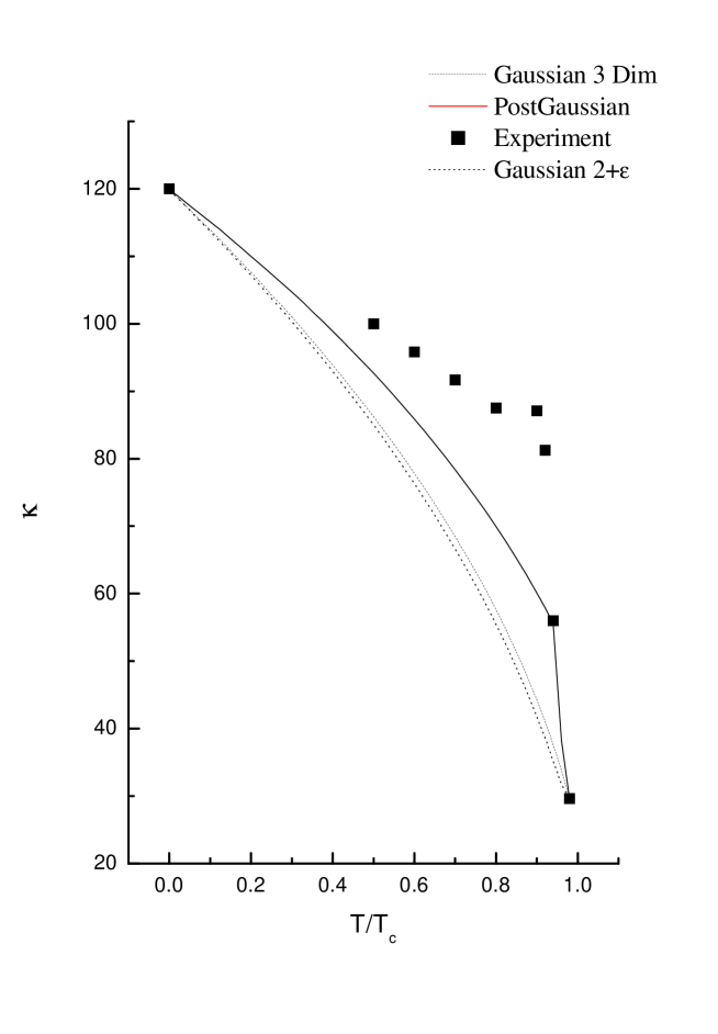
FIG. 1.: The GL parameter, $\kappa$, in the Gaussian approximation in $D=3$ (the dotted line) and $D=2+\varepsilon$ (the dashed line) cases. The solid line represents the PostGaussian approximation for $D=3$ case.

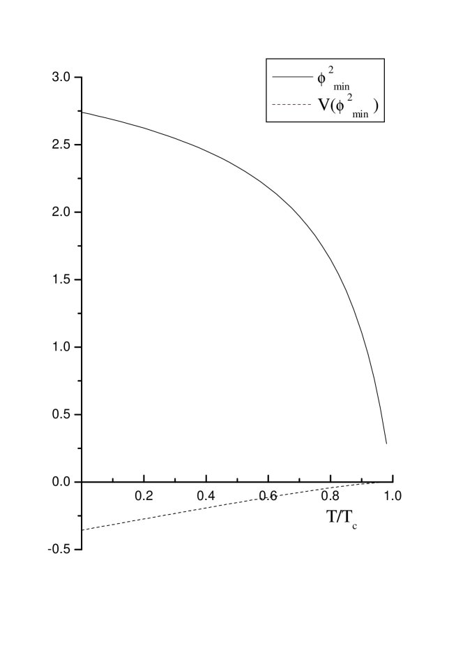
FIG. 2.: The stationary point $\bar{\phi}_{0}^{2}$ and the depth of the post Gaussian effective potential at the stationary point vs. temperature.

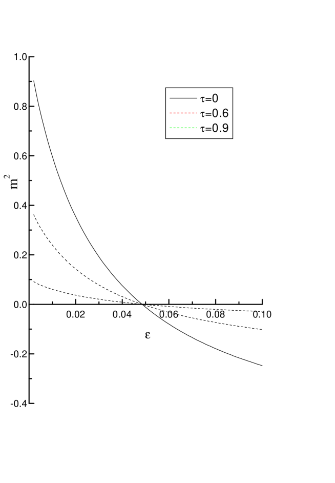
FIG. 3.: The parameter $m^{2}$ of th GL model given by Eqs. (79) and (91) for $D=2+2\varepsilon$.

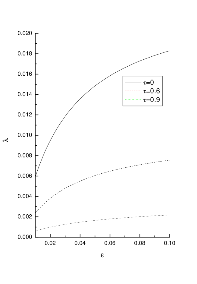
FIG. 4.: The same as in Fig.3 but for $\lambda$

REFERENCES

- [1] V. L. Ginzburg and L.D. Landau, Zh. Eksp. Teor. Fiz. 20, 1064, (1950) .
- [2] L.P. Gorkov, Sov. Phys. JETP 7, 505 (1958); L.P. Gorkov, Sov. Phys. JETP 9, 1364 (1959).
- [3] Z. Tesanovich, Phys. Rev. B59, 6449, (1999) (and references there in).
- [4] A. K. Nguyen and A. Sudbo, Phys. Rev. B60 15307 (1999).
- [5] M. Camarda, G.G.N. Angilella, R. Pucci and F. Siringo , Eur.Phys.J. B33 , 273, (2003).
- [6] L.M. Abreu, A.P.C. Malbouisson and I. Roditi ”GAUGE FLUCTUATIONS IN SUPERCONDUCTING FILMS.” cond-mat/0305366.
- [7] I. Stancu and P. M. Stevenson, Phys. Rev. D42, 2710, (1990).
- [8] H. Kleinert, Gauge Fields in Condensed Matter, Vol. 1: Superflow and Vortex Lines, World Scientific , Singapore,1989.
- [9] A. Rakhimov and J.H. Yee, Int. J. Mod. Phys. A19, 1589 ( 2004).
- [10] G.H. Lee and J.H. Yee, Phys. Rev. D56, 6573, (1997).
- [11] E. Braaten and A. Nieto, Phys. Rev. D51, 6990, (1995); A. I. Davydychev and M. Yu. Kalmykov Nucl. Phys. B605, 266, (2001); A. K. Rajantie Nucl. Phys. B480, 729, (1996).
-
[12]
G. Brandstatter, F.M. Sauerzopf, H. W. Weber, F. Ladenberger
and E. Schwarzmann, Physica C, 235, 1845, (1994);
G. Brandstatter, F.M. Sauerzopf and H. W. Weber, Phys. Rev. B55, 11693, (1997). - [13] S. Chiku and T. Hatsuda Phys. Rev. D58, 076001, (1998).
- [14] N. Banerjee and S. Malik Phys. Rev. D43,3368, (1991).