Microcanonical entropy for small magnetisations

Abstract

Physical quantities obtained from the microcanonical entropy surfaces of classical spin systems show typical features of phase transitions already in finite systems. It is demonstrated that the singular behaviour of the microcanonically defined order parameter and susceptibility can be understood from a Taylor expansion of the entropy surface. The general form of the expansion is determined from the symmetry properties of the microcanonical entropy function with respect to the order parameter. The general findings are investigated for the four-state vector Potts model as an example of a classical spin system.

1 Introduction

The macroscopic behaviour of a physical system in thermodynamic equilibrium is related to the microscopic properties by statistical mechanics. The basic quantity in this connection is the density of states depending on the macroscopic quantities of interest. For a classical spin system as a model system to describe magnetic properties these macroscopic variables are the energy and the magnetisation. In the traditional approach to the statistical description of phase transitions the density of states is Laplace-transformed to the partition function which is a concept of the canonical ensemble and the physics is deduced from the corresponding potential, the Gibbs free energy. In recent years an alternative approach to analyse phase transitions within a statistical framework has been developed in the microcanonical ensemble (Gross, 1986a; 1986b; 2001; Hüller, 1994; Promberger/Hüller, 1995; Gross et al., 1996). Apart from works about general questions of the equivalence and inequivalence of the various ensembles (Lewis et al., 1994; Dauxois et al., 2000; Barré et al., 2001; Ispolatov/Cohen, 2001) and of the thermodynamic limit in the microcanonical ensemble ((Kastner 2002) to cite a recent work) also second order phase transitions have been studied recently (Kastner et al., 2000; Hüller/Pleimling, 2002). Ways to extract critical exponents from microcanonical quantities have been suggested (Kastner et al., 2000; Hüller/Pleimling, 2002). In these works is was numerically demonstrated that the microcanonically defined physical quantities like the microcanonical order parameter or the susceptibility exhibit singularities already in finite systems. However, these numerical studies suggest that the microcanonical singularities are characterised by classical critical exponents in contrast to the non-trivial exponents showing up in the thermodynamic limit.

The aim of the present paper is to provide an analytic understanding of the characterisation of the singularities in physical quantities of finite microcanonical systems by classical exponents. To this end the entropy surface is expanded into a Taylor series in terms of its natural variables energy and magnetisation and the asymptotic behaviour of the macroscopic quantities is investigated. This procedure is similar to the Landau expansion of the free energy of the infinite system although a striking difference has to be stressed. The Landau approach is an approximation of the free energy of the infinite canonical system whereas the treatment presented below is exact for the finite microcanonical system.

The work is organised in the following way. The second section contains a short survey of the microcanonical approach to statistical mechanics. In particular the basic concepts and findings of the investigation of second order phase transitions are summarised. In the third section the appearance of the classical critical exponents is related to the analyticity of the thermodynamic potential of finite systems. The fourth section contains general considerations about the Taylor expansion of entropy surfaces with a $C_{nv}$ order parameter symmetry. In addition an investigation of the entropy surface of finite vector Potts models with four states is presented. The analysed data are obtained from Monte Carlo simulations.

2 Thermostatics in microcanonical systems

The analysis of statistical properties of classical spin systems within the microcanonical ensemble starts from the density of states

$$\Omega(E,M,L^{-1})=\sum_{\sigma\in\Gamma_{N}}\delta_{E,\mathcal{H}(\sigma)}\delta_{M,\mathcal{M}(\sigma)}\;.$$ (1)

Here it is assumed that the system is defined on a $d$-dimensional hypercube of extension $L$. The Hamiltonian $\mathcal{H}$ gives the total energy of the microstate $\sigma$ and the magnetisation operator $\mathcal{M}$ its total magnetisation. In general the magnetisation is a multicomponent object $M=(M_{1},\ldots,M_{n})$. The microcanonical entropy is obtained by taking the logarithm of the density of states:

$$s(e,m,L^{-1})=\frac{1}{L^{d}}\ln\Omega(E,M,L^{-1})\;.$$ (2)

To compare different system sizes the extensive factor $L^{d}$ is divided out to give the specific energy $e=E/L^{d}$ and the specific magnetisation $m=M/L^{d}$. The dependence of the physical quantities on the system size $L$ is suppressed in the following. The statistical properties of an isolated physical system are deduced from the entropy surface. The microcanonical spontaneous magnetisation of a finite system for a fixed energy is defined by

$$m_{\scriptsize\mbox{sp}}(e):\iff s(e,m_{\scriptsize\mbox{sp}}(e))=\max_{m}s(e,m)\;,$$ (3)

hence $m_{\scriptsize\mbox{sp}}(e)$ corresponds to the magnetisation with the maximum entropy for a given energy.

The non-vanishing multicomponent spontaneous magnetisation vector defines a direction in the order parameter space:

$$m_{\scriptsize\mbox{sp}}(e)=(m_{\scriptsize\mbox{sp}}^{(1)}(e),\ldots,m_{\scriptsize\mbox{sp}}^{(n)}(e))=|m_{\scriptsize\mbox{sp}}(e)|m_{0}$$ (4)

where $m_{0}$ is a fixed unit vector with several possible orientations below $e_{\scriptsize\mbox{c}}$. Note however that it might be possible that $m_{0}$ and consequently the associated orientations are themselves functions of the energy below $e_{\scriptsize\mbox{c}}$. Let $G_{0}$ be the symmetry group of the microcanonical entropy with respect to the magnetisation components, i.e.

$$s(e,g(m))=s(e,m)$$ (5)

for all transformations $g$ in $G_{0}$. If the spontaneous magnetisation $m_{\scriptsize\mbox{sp}}$ is finite the symmetry group $G_{0}$ of the entropy is broken down to the subgroup $G<G_{0}$ that leaves the direction $m_{0}$ invariant (Behringer, 2003).

In the microcanonical ensemble of isolated systems no external magnetic field appears. However, magnetic fields can be defined as the conjugated variable of the magnetisation components giving rise to the relation

$$h_{i}(e,m_{\scriptsize\mbox{sp}}(e))\frac{\partial}{\partial e}s(e,m_{\scriptsize\mbox{sp}}(e))=-\frac{\partial}{\partial m_{i}}s(e,m_{\scriptsize\mbox{sp}}(e))$$ (6)

for the $i$th component in equilibrium.

The susceptibility of the system is related to the curvature of the entropy along the magnetisation direction. For a multicomponent magnetisation the curvature at the spontaneous magnetisation is related to the Hessian

$$H_{kl}(e,m_{\scriptsize\mbox{sp}}(e))=\frac{\partial^{2}}{\partial m_{k}\partial m_{l}}s(e,m_{\scriptsize\mbox{sp}}(e))$$ (7)

of the entropy and the susceptibility is consequently a tensor which is given by

$$\chi^{(0)}_{ij}(e)=-\frac{\partial}{\partial e}s(e,m_{\scriptsize\mbox{sp}}(e))\left(H^{-1}(e,m_{\scriptsize\mbox{sp}}(e))\right)_{ij}\;.$$ (8)

From a geometrical point of view the specific heat of the system is connected to the curvature along the energy direction. At the spontaneous magnetisation the specific heat is given by

$$c^{(0)}(e)=-\frac{\left(\frac{\partial}{\partial e}s(e,m_{\scriptsize\mbox{sp}}(e))\right)^{2}}{\frac{\partial^{2}}{\partial e^{2}}s(e,m_{\scriptsize\mbox{sp}}(e))}\;.$$ (9)

Alternatively one can consider a specific heat that is more directly related to the canonical viewpoint. There the specific heat is calculated from the canonical entropy

$$s_{\scriptsize\mbox{can}}=-\frac{\partial}{\partial T}g(T,h)$$ (10)

obtained from the Gibbs free energy $g(T,h)$ of the system in equilibrium as

$$c_{\scriptsize\mbox{can}}=T\frac{\partial}{\partial T}s_{\scriptsize\mbox{can}}\;.$$ (11)

Defining the equilibrium entropy by

$$\tilde{s}(e)=s(e,m_{\scriptsize\mbox{sp}}(e))$$ (12)

one obtains the alternative specific heat

$$\tilde{c}(e)=-\frac{\left(\frac{\mbox{d}}{\mbox{d}e}\tilde{s}(e)\right)^{2}}{\frac{\mbox{d}^{2}}{\mbox{d}e^{2}}\tilde{s}(e)}\;.$$ (13)

The specific heat $\tilde{c}$ is different from $c^{(0)}$ as $m_{\scriptsize\mbox{sp}}$ is first plugged into $s$ and the derivative with respect to the energy is worked out afterwards. In contrast, $c^{(0)}$ is evaluated according to footnote $\ddagger$.

From a statistical point of view a phase transition from a disordered high-symmetric macrostate to an ordered low-symmetric macrostate is defined to take place at a non-analytic point of the corresponding thermostatic potential describing the properties of the physical system. Yang and Lee showed that the grand-canonical thermostatic potential, i.e. the Gibbs free energy, is an analytic function for all finite system sizes (Yang/Lee, 1952; Lee/Yang, 1952). This means that a phase transition can only occur in the thermodynamic limit of an infinite system, according to the definition above phase transitions are not possible in finite systems.

However the microcanonical equilibrium quantities exhibit typical features of phase transitions (Kastner et al., 2000). For instance the microcanonical spontaneous magnetisation (3) displays the characteristics of spontaneous symmetry breaking. This spontaneous magnetisation defines the order parameter. For the high energy phase the microcanonical order parameter is zero reflecting a phase with high symmetry. The abrupt emerging of a finite order parameter for low energies indicates the transition to an ordered phase with lower symmetry. The energy at which this onset occurs defines unambiguously the critical energy $e_{\scriptsize\mbox{c}}$ of the finite microcanonical system. The susceptibility (8) of the system diverges at this energy.

The use of the expressions critical and phase transition to describe the behaviour of finite microcanonical systems is somewhat problematic as they are commonly used for certain properties of the infinite system. Nevertheless the appearance of features of the microcanonical quantities which are also found in infinite systems at the transition point suggests its usage. Another delicate point is the discreteness of the physical quantities of discrete spin systems. There the used language refers to continuous functions that describe the discrete data most suitably. In the microcanonical analysis of continuous spin systems as e.g. the $xy$ (Richter et al., 2004) or the Heisenberg model this concern does not exist.

The existence of a nontrivial spontaneous magnetisation is in general related to the appearance of a convex dip in the microcanonical entropy. This is different in the canonical ensemble where the curvature along the natural variables is connected to the mean square deviation of a physical quantity. The curvature has therefore a well-defined sign. Although the physical quantities show singularities at the transition point that are typical of phase transitions there is no phase transition as long as the microcanonical system is finite. The microcanonical entropy of finite systems is an analytic function of its natural variables and hence a phase transition in the above defined mathematical sense does not take place.

The singular behaviour of the order parameter with respect to the energy can, however, be described by means of a critical exponent (Kastner et al., 2000). For a physical quantity $Q(e)$ of the finite system this critical exponent, say $\tilde{\kappa}$, is defined by

$$\tilde{\kappa}=\lim_{e\to e_{\scriptsize\mbox{c}}}\frac{\mbox{d}\ln|Q(e)|}{\mbox{d}\ln|e-e_{\scriptsize\mbox{c}}|}\;.$$ (14)

The microcanonical critical exponent $\tilde{\beta}$ of the spontaneous magnetisation in finite systems turns out to have the classical value 1/2, the corresponding exponent $\tilde{\gamma}$ of the susceptibility is 1 for all system sizes. Both definitions (9) and (13) of the specific heat are characterised by the exponent $\tilde{\alpha}=0$. Whereas the specific heat $c^{(0)}$ has a kink at the critical energy, $\tilde{c}$ exhibits a jump at $e_{\scriptsize\mbox{c}}$ with different values $\tilde{c}(e_{c}^{+})\neq\tilde{c}(e_{c}^{-})$. The kink of $c^{(0)}$ at the critical energy with $c^{(0)}(e_{c}^{+})=c^{(0)}(e_{c}^{-})$, but different left-handed and right-handed derivatives at $e_{c}$, however, is not a cusp-singularity according to the definition of (Stanley, 1972) as the higher order derivatives of $c^{(0)}$ do not diverge at $e_{\scriptsize\mbox{c}}$. Note also that both quantities tend to the same function in the thermodynamic limit.

3 Taylor expansion of the microcanonical entropy

For a finite system with the typical characteristics of a continuous phase transition the microcanonically defined order parameter near the critical point vanishes like a square root. This behaviour can be understood in a Landau type of approach to the description of phase transitions in the microcanonical ensemble. To this end the entropy is expanded into a Taylor series as a function of the order parameter components. A proof of the analyticity of the microcanonical entropy is still lacking. Nevertheless in view of the analyticity of the canonical thermostatic potential it seems obvious to use this assumption. Note that this approach is exact provided the entropy of a finite system is an analytic function and hence can be expanded about any point $(e,m)$ in the parameter space. This is different in the Landau theory of the free energy of the infinite system. In this approximation the Helmholtz free energy is assumed to be analytic although a phase transition in the thermodynamic limit is related to a non-analytic point in the thermostatic potential. Consequently the critical behaviour obtained from the Landau approximation may differ from the true non-trivial behaviour of the physical systems. This is indeed the case below the upper critical dimension.

The Taylor expansion of the microcanonical entropy of the finite system about the magnetisation $m=0$ (the equilibrium magnetisation of the high energy phase) yields the general series

$$s(e,m)=s(e,m=0)+\sum_{(p_{1},\ldots,p_{n})}a_{p_{1},\ldots,p_{n}}(e)\prod_{i}m_{i}^{p_{i}}\;,$$ (15)

where the expansion coefficients are related to the derivatives of the entropy with respect to the magnetisations

$$a_{p_{1},\ldots,p_{n}}(e)=\frac{1}{p_{1}!\ldots p_{n}!}\partial^{p_{1}}_{m_{1}}\ldots\partial^{p_{n}}_{m_{n}}s(e,m=0)\;.$$ (16)

The symmetry group $G_{0}$ of the entropy with respect to the magnetisation determines which coefficients $a_{p_{1},\ldots,p_{n}}$ appear in the expansion (15). Only the coefficients which correspond to monomials $m_{1}^{p_{1}}\ldots m_{n}^{p_{n}}$ that are invariant under the transformations $g\in G_{0}$ are in general non-zero, all other coefficients necessarily vanish. In view of the symmetry $G_{0}$ the expansion (15) is in fact an expansion in terms of the symmetry-adapted harmonics of the group $G_{0}$.

The physical behaviour for small magnetisations is already described by the low order terms in (15). Suppose the magnetisation is only one-dimensional and the microcanonical entropy is left invariant by the transformation $m\to-m$. Note that these are the symmetry properties of the entropy of the Ising model. Then only even powers contribute to the Taylor expansion and up to the fourth order term one gets

$$s(e,m)=s(e,0)+\frac{1}{2}a(e)m^{2}+\frac{1}{4}b(e)m^{4}.$$ (17)

As the maximum of the entropy must not be at an infinite magnetisation the coefficient of the highest power of $m$ has to be negative. This requirement is indeed fulfilled for an Ising model in the energy interval about $e_{\scriptsize\mbox{c}}$ where a finite order parameter emerges. The Ising model is defined by the Hamiltonian

$$\mathcal{H}=-\sum_{\left<ij\right>}\sigma_{i}\sigma_{j}$$ (18)

where the spins $\sigma_{i}$ can be in the state $+1$ or $-1$ and the summation runs over neighbour pairs of spins. Figure 1 displays the derivatives $\partial_{m^{q}}s(e,0)$ of a two-dimensional Ising model with 200 spins near the energy $e_{\scriptsize\mbox{c}}$. The underlying two-dimensional lattice has a square-lattice topology. The density of states of the system is evaluated numerically exact by a microcanonical transfer matrix method (Binder, 1972; Creswick, 1995) so that it is possible to work out higher order derivatives reliably. The condition (3) for thermostatic equilibrium leads to the equation

$$\frac{\partial}{\partial m}s(e,m)=m\left(a(e)+b(e)m^{2}\right)\stackrel{{\scriptstyle}}{{=}}0\;.$$ (19)

for $m_{\scriptsize\mbox{sp}}(e)$. This relation has always the trivial solution $m_{\scriptsize\mbox{sp}}(e)=0$ and in addition the solutions

$$m_{\scriptsize\mbox{sp}}(e)=\pm\sqrt{-\frac{a(e)}{b(e)}}$$ (20)

with a non-trivial, finite order parameter if the coefficient $a(e)$ is positive. The stability condition

$$\frac{\partial^{2}}{\partial m^{2}}s(e,m_{\scriptsize\mbox{sp}}(e))\stackrel{{\scriptstyle}}{{<}}0$$ (21)

is always satisfied for the non-trivial solution (20) provided it exists. The solution $m_{\scriptsize\mbox{sp}}(e)=0$ is only stable, i.e. corresponds to a maximum of the entropy, if the coefficient $a(e)$ is negative. The coefficient $a(e)$ changes its sign at the energy $e_{\scriptsize\mbox{c}}$. Hence the equilibrium magnetisation of the entropy (17) is given by

$$m_{\scriptsize\mbox{sp}}(e)=\pm\Theta(a(e))\sqrt{\left|\frac{a(e)}{b(e)}\right|}\;,$$ (22)

where the Heaviside function is denoted by $\Theta$. As the coefficient $b(e)$ is negative in the vicinity of $e_{\scriptsize\mbox{c}}$ and the two functions $a$ and $b$ are smooth the order parameter varies continuously as a function of the energy $e$. Below the energy $e_{\scriptsize\mbox{c}}$ it attains a finite value. Note that at the energy $e_{\scriptsize\mbox{c}}$ the solution $m=0$ becomes instable and the curvature of the entropy along the magnetisation changes its sign. The existence of two stable solutions below $e_{\scriptsize\mbox{c}}$ signals the spontaneous breakdown of the global $m\to\pm m$ symmetry of the physical system. The depth

$$\Delta(e)=s(e,m_{\scriptsize\mbox{sp}}(e))-s(e,0)$$ (23)

of the convex dip along the magnetisation for fixed energy can also be expressed in terms of the expansion coefficients of the entropy surface. Near the critical point of the finite system one obtains the approximation

$$\Delta(e)\approx-\Theta(a(e))\frac{a^{2}(e)}{4b(e)}\;.$$ (24)

The Landau expansion of the entropy surface around the equilibrium magnetisation of the high energy phase provides an explanation of the classical exponents describing the singular behaviour of the microcanonical physical quantities of the finite system. Introducing the reduced energy

$$\varepsilon:=e-e_{\scriptsize\mbox{c}}$$ (25)

one can expand the functions $a(e)$ and $b(e)$ about the critical energy $e_{\scriptsize\mbox{c}}$:

$$a(e)=-A\varepsilon+a_{2}\varepsilon^{2}+\ldots$$ (26)

and

$$b(e)=-B+b_{1}\varepsilon+b_{2}\varepsilon^{2}+\ldots$$ (27)

where the constants $A$ and $B$ are positive. Plugging these expansions into relations (22) and (24) one gets the leading behaviour

$$m_{\scriptsize\mbox{sp}}(\varepsilon)=\pm\Theta(-\varepsilon)\sqrt{\frac{A}{B}}\sqrt{|\varepsilon|}$$ (28)

for the order parameter and

$$\Delta(\varepsilon)=\Theta(-\varepsilon)\frac{A^{2}}{4B}\varepsilon^{2}$$ (29)

for the depth of the convex dip in the limit of small reduced energies $\varepsilon$. Thus the variation of the spontaneous magnetisation in finite systems is described by the classical critical exponent $\tilde{\beta}=1/2$. In addition one can deduce the leading behaviour of the curvature of the entropy along the magnetisation. For energies above the critical point, i.e. $\varepsilon>0$ one has

$$\partial_{mm}s(\varepsilon,m_{\scriptsize\mbox{sp}}(\varepsilon))=-A\varepsilon$$ (30)

and for negative reduced energies one has

$$\partial_{mm}s(\varepsilon,m_{\scriptsize\mbox{sp}}(\varepsilon))=2A\varepsilon\;.$$ (31)

This leads to the critical exponent $\tilde{\gamma}=1$ characterising the divergent susceptibility in finite microcanonical systems. Note that the slope of the curvature $\partial_{mm}s$ at the spontaneous magnetisation above and below the critical point differ by a factor two. This is also observed in the curves obtained from the numerically calculated entropy surface (see discussion below and figure 5). From the definition (6) of the magnetic field and the expansion (17) it is apparent that the magnetic field at the critical energy $e_{\scriptsize\mbox{c}}$ vanishes with an exponent $\tilde{\delta}=3$ in the limit of small magnetisations. Similarly the critical exponent $\tilde{\alpha}$ can be shown to be $0$ for both definitions of the specific heat (compare (9) and (13)).

The expansion of the entropy surface hence describes the asymptotic behaviour of the physical quantities in the vicinity of the critical point of the finite system. It has to be stressed once again that the expansion of the entropy surface is not an approximation like the Landau expansion of the Helmholtz free energy. The Taylor expansion of the microcanonical entropy about an arbitrary point in the $(e,m)$ space is always possible due to the analyticity of the entropy of finite systems. For the infinite system such an expansion about the critical point can not be performed as the thermostatic potential is singular precisely at this point. Therefore non-trivial critical exponents can only emerge in the thermodynamic limit.

Although the physical quantities of finite microcanonical systems are always characterised by classical exponents precursors of the non-trivial exponent of the infinite system show up if the evolution of the quantities is considered for a series of different system sizes. This evolution of the physical quantities with increasing size $L$ can be investigated with effective critical exponents (Hüller/Pleimling, 2002) or microcanonical finite size scaling relations (Kastner et al., 2000). The microcanonical finite size scaling theory is conceptionally similar to the corresponding finite size scaling theory of the canonical ensemble.

At this stage one delicate point has to be stressed again. Whereas the Taylor expansion of the entropy can be carried out without any ambiguity for systems with continuous energies and magnetisations (e.g. $xy$ model) this seems to be doubtful for discrete models such as the Ising model. A suitable chosen continuous function may be fitted to the data. This leads, however, to a certain degree of arbitrariness which is still related to the choice of this function. Alternatively, differentials can be replaced by (centre) differences leading to a discrete set of data points. Nevertheless, any properly chosen function will reproduce the change of the curvature along the magnetisation at $m=0$ and $e_{\scriptsize\mbox{c}}$, leading to maxima at non-zero magnetisations. It is precisely this bifurcation at $e_{\scriptsize\mbox{c}}$ that gives rise to classical exponents. Different fit-functions will only lead to slightly different coefficients, the overall dependence of the expansion an $e$ and $m$ will be the same. The considerations in this section strictly valid only for systems with continuous $e$ and $m$ give a heuristic understanding of the classical behaviour of physical quantities of discrete systems.

4 Entropy surface with $C_{nv}$ symmetry

4.1 Landau expansion of entropies with $C_{nv}$ invariance

A general method that allows the determination of the invariant homogeneous polynomials which can appear in the Taylor expansion of the entropy is based on the concept of the complete rational basis of invariants of a group. The determination of the Landau expansion of the free energy of an infinite system with the help of the complete rational basis of invariants was first proposed by Gufan in (Gufan, 1971) (see also Tolédano/Tolédano, 1987). In this subsection this general method is applied to a microcanonical entropy surface with a $C_{nv}$ symmetry. A prominent example of a physical system with this symmetry property of the entropy surface is the $n$-state vector Potts model which will be investigated in section 4.2 for a two-dimensional lattice.

An invariant homogeneous monomial of degree $p$ with respect to a finite group can be constructed as a linear combination of products of a limited number of polynomials forming the complete rational basis of invariants. In polar coordinates $m_{1}=r\cos\phi$ and $m_{2}=r\sin\phi$ the complete rational basis of invariants of the finite group $C_{nv}$ consists of the two polynomials $r^{2}$ and $r^{n}\cos n\phi$. The polynomial $r^{2}=m_{1}^{2}+m_{2}^{2}$ is always invariant under the modulus preserving transformations of the group $C_{nv}$.

The entropy of a finite microcanonical system with the symmetry

$$s(e,m_{1},m_{2})=s(e,C_{nv}(m_{1},m_{2}))$$ (32)

can be expanded into a Taylor series. In polar coordinates the polynomials appearing in the expansion are sums of products of the monomials of the rational basis of invariant of $C_{nv}$. The basic monomials contain the angular dependence of the magnetisation exclusively in the form $\cos n\phi$. Thus the entropy in polar coordinates is of the form

$$s(e,m_{1},m_{2})=\tilde{s}(e,r,\cos n\phi)\;.$$ (33)

This form of the entropy already determines properties that are independent of the details of the Taylor expansion, as e.g. the highest degree in the truncated Taylor series. These properties are solely a consequence of the symmetry of the entropy. With $b=\cos n\phi$ the equilibrium equations are

$$\frac{\partial}{\partial r}\tilde{s}(e,r,b)\stackrel{{\scriptstyle}}{{=}}0$$ (34)

for the modulus of the spontaneous magnetisation and

$$\sin(n\phi)\frac{\partial}{\partial b}\tilde{s}(e,r,b)\stackrel{{\scriptstyle}}{{=}}0$$ (35)

for its angular dependence. The equilibrium condition for the angular part can be satisfied in two ways. Either the derivative $\partial_{b}\tilde{s}$ vanishes or $\sin n\phi$ is zero. The latter is the case for $\phi=k\pi/n$ with $k=0,\ldots,2n-1$. The former way to satisfy equation (35) is discussed in section 4.3. The stability of the solution of (34) and (35) requires that the corresponding Hessian is a negative definite matrix. Suppose that the stability is guaranteed for the radial order parameter component, i.e. $\partial_{rr}\tilde{s}<0$. At $\phi=k\pi/n$ the Hessian in polar coordinates reduces to

$$H\left(e,\phi=k\pi/n\right)=\left(\begin{array}[]{cc}\frac{\partial^{2}}{\partial r^{2}}\tilde{s}&0\\ 0&-\frac{n^{2}}{r^{2}}(-1)^{k}\frac{\partial}{\partial b}\tilde{s}\end{array}\right)$$ (36)

and hence the negativity of $H$ is satisfied if $(-1)^{k}\partial_{b}\tilde{s}>0$. The factor $(-1)^{k}$ can either be $+1$ or $-1$ leading to maxima or saddle points of the microcanonical entropy surface at the solutions of the equilibrium conditions (34) and (35). For a positive $\partial_{b}\tilde{s}$ the spontaneous magnetisation can have the orientations $\phi=k\pi/n$ with even $k$. In this situation the extrema on directions with odd $k$ are saddle points of the entropy surface.

These considerations show that the direction of the spontaneous magnetisation of an entropy with $C_{nv}$ invariance is already determined from the symmetry properties with respect to the magnetisation. The extrema of the entropy appear along the symmetry lines of the associated regular $n$-polygon in the magnetisation plane.

To get further information about the behaviour of the entropy surface for small magnetisations a Taylor expansion must actually be performed. The precise form of this Taylor expansion, i.e. the expansion coefficients and the degree of the truncated Taylor polynomial determines the stability of the extrema and the form of the energy dependence of the actual order parameter $r_{\scriptsize\mbox{sp}}(e)=|m_{\scriptsize\mbox{sp}}(e)|$. To ensure the stability in angular direction one must have $\partial_{b}\tilde{s}\neq 0$ and hence the Taylor expansion has to contain at least the $n$th degree monomial $r^{n}b=r^{n}\cos n\phi$.

4.2 Entropy of the four-state vector Potts model

The general results of the previous subsection can be illustrated for an entropy with $C_{4v}$ symmetry in the magnetisation space. The rational basis of invariants is then given by $\{r^{2},r^{4}\cos 4\phi\}$ and the Taylor expansion of the entropy $s(e,r,\phi)$ up to the fourth degree term has the general form

$$s(e,r,\phi)=s_{0}(e)+\frac{1}{2}A(e)r^{2}+\frac{1}{4}B(e)r^{4}+\frac{1}{4}C(e)r^{4}\cos 4\phi\;.$$ (37)

To ensure the appearance of a stable extremum for finite magnetisations the coefficients of the fourth degree term have to satisfy $B(e)+C(e)\cos 4\phi<0$ for all angles $\phi$. The extrema of the entropy are along the symmetry directions $\phi=k\pi/4$ with $k=0,\dots,7$ of the square in the two-dimensional plane. The stability in angular direction requires that the inequality

$$C(e)\cos k\pi>0$$ (38)

is satisfied. For a positive coefficient $C(e)$ this has the consequence that the maxima of the microcanonical entropy surface lie on the directions $\phi\in\{0,\pi/2,\pi,3\pi/2\}$ provided the stability of the radial order parameter is ensured. The extrema on the four remaining symmetry directions correspond to saddle points in the entropy function.

An example of a classical spin model with $C_{4v}$ symmetry is the vector Potts model (Wu, 1982) with four states whose Hamiltonian is given by

$$\mathcal{H}=-\sum_{\left<i,j\right>}\cos\left(\frac{\pi}{2}(k_{i}-k_{j})\right)\;.$$ (39)

The spins $k_{i}$ can take on the values 1, 2, 3 and 4 and be visualised by unit vectors with the orientations $0$, $\pi/2$, $\pi$ and $3\pi/2$ in a two-dimensional plane. The intensive magnetisation of the system with $N$ spins is given by

$$m_{1} = \frac{1}{N}\sum_{i}\cos\left(\frac{\pi}{2}k_{i}\right)$$ (40)

$$m_{2} = \frac{1}{N}\sum_{i}\sin\left(\frac{\pi}{2}k_{i}\right)\;.$$ (41)

The system has four equivalent ground states with the spontaneous magnetisations $(1,0)$, $(0,1)$, $(-1,0)$ and $(0,-1)$. These four ground state magnetisations define a square in the magnetisation plane.

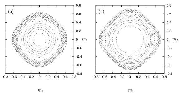
Figure 2: Level curves of the density of states of the four-state vector Potts model with $64$ spins in two dimensions for the two energies $-0.91$ (a) and $-1.06$ (b) below the critical point $e_{\scriptsize\mbox{c}}=-0.7\pm 0.005$. Four equivalent maxima appear along the bisectors of the square defined by the ground state magnetisations.

For a two-dimensional system with a finite number of spins the entropy has one single maximum at zero magnetisation above the critical energy $e_{\scriptsize\mbox{c}}$. Below $e_{\scriptsize\mbox{c}}$ the entropy has four equivalent maxima along the directions defined by the coordinate axes. The extrema on the diagonals of the coordinate system correspond to saddle points of the entropy surface. In figure 2 the level curves of the entropy of a two-dimensional system with $64$ spins are shown for two energies below the critical one. The data are calculated with the transition observable method that allows a highly efficient and accurate determination of microcanonical entropy surfaces (Hüller/Pleimling, 2002). The findings show that the angular equilibrium equation (35) is satisfied by the condition $\sin 4\phi=0$ for the four-state vector Potts model. The appearance of stable phases along the coordinate axes suggests that the coefficient $C(e)$ is indeed positive. However it is hardly possible to obtain a reliable estimate of the fourth derivative from an entropy that has been calculated by means of Monte Carlo simulations. A direct determination of the expansion coefficients $B(e)$ and $C(e)$ is therefore not possible. To get an impression of the values of these coefficients one can use an indirect approach. The coefficient $A(e)$ of the second degree term in the expansion (37) is determined by differentiating the entropy. The coefficients $B(e)\pm C(e)$ corresponding to the direction $0$ and $\pi/2$ are then varied to achieve a good description of the data by the fourth degree expansion for small magnetisations. For the energy $-0.75$ near $e_{\scriptsize\mbox{c}}=-0.7$ this gives for the system with $L=8$ the value $-1.14$ for $B$ and the positive value $0.04$ for $C$ in agreement with the general considerations above. For a system with $L=10$ this procedure yields the coefficients $B=-0.804$ and the positive value $0.048$ for $C$ at the energy $-0.86$ below the critical energy $-0.806\pm 0.005$. Note however that this procedure may lead to large errors due to the subjective assessment of the agreement of the Taylor polynomial with the data for small magnetisations. The simulated entropy for the system with $100$ spins together with its fourth degree Taylor approximation along the $m_{1}$ direction is displayed in figure 3.

The behaviour of the spontaneous magnetisation of the two-dimensional system with $64$ spins resulting from the variation of the position of the maximum is displayed in figure 4. Its energy dependence near the critical energy $e_{\scriptsize\mbox{c}}=-0.7$ is most suitably characterised by a square root behaviour, i.e. by the exponent $\tilde{\beta}=1/2$. This can be understood from the general considerations in section 3. The non-zero spontaneous magnetisation $m_{sp}(e)$ defines a vector in the order parameter space with a energy-dependent modulus $|m_{sp}(e)|$ and a fixed, energy-independent direction $m_{0}$ (compare relation (4)). Once the direction $m_{0}$ has been chosen, e.g. along the $m_{1}$ axis, the entropy depends only on the modulus $|m|$ leading to an entropy function with a one-dimensional order parameter. This function is just the cut of the entropy surface along the $m_{0}$ direction. The expansion of this function with respect to $|m|$ can be performed as in section 3 and yields the characteristic asymptotic square root energy behaviour of the microcanonical equilibrium magnetisation of finite systems near the transition energy $e_{\scriptsize\mbox{c}}$. The curvature parallel to the spontaneous magnetisation at the equilibrium macrostate of the system with $100$ spins near the critical point is shown in figure 5. It results in a diverging susceptibility characterised by the critical exponent $\tilde{\gamma}=1$. The amplitudes from the left and from the right differ approximately by a factor $2$. These observations are in agreement with the general findings obtained by Taylor expanding the microcanonical entropy surface. Note however that the susceptibility of the four-state vector Potts model is a tensor. Due to the symmetry (32) of the entropy surface the susceptibility tensor is diagonal with a non-vanishing parallel and perpendicular component with respect to the equilibrium magnetisation. The behaviour of the depth of the convex dip of the entropy surface below the critical energy $e_{\scriptsize\mbox{c}}$ is shown in figure 6 for the system with $100$ spins. Once again the parabolic energy dependence suggested by the above considerations is confirmed.

4.3 Energy-dependent angular magnetisation

To complete the discussion of the angular equilibrium equation (35) this section focuses on the possible solution $\partial_{b}\tilde{s}=0$. The derivative $\partial_{b}\tilde{s}$ contains the radial magnetisation so that the two equilibrium equations for $r_{\scriptsize\mbox{sp}}$ and $\phi_{\scriptsize\mbox{sp}}$ are coupled. This set of equations can be solved for $b$ and gives $b_{\scriptsize\mbox{sp}}$ or equivalently $\phi_{\scriptsize\mbox{sp}}$ as a function of $r_{\scriptsize\mbox{sp}}$ and hence it will depend on the energy. Consequently The direction of the spontaneous magnetisation exhibits an energy dependence. This dependence on the energy is influenced by the precise form of the truncated Taylor expansion which determines the order parameter as a function of the energy. The stability of the extremum requires additionally that the expansion must contain monomials up to the degree $2n$ at least. To see this consider the component $H_{\phi\phi}$ of the Hessian which is given by

$$H_{\phi\phi}^{(0)}=\frac{n^{2}}{r_{\scriptsize\mbox{sp}}^{2}}(\sin n\phi_{\scriptsize\mbox{sp}})^{2}\partial_{bb}\tilde{s}$$ (42)

at the spontaneous magnetisation. This requirements for the Taylor expansion has the further consequence that the phase diagram with respect to the expansion coefficients of the entropy allows only an isolated continuous transition (Gufan/Sakhnenko, 1973).

The author does not know of any model system that exhibits an energy-dependent orientation of the microcanonically defined order parameter. Nevertheless, the general statements of this section can be illustrated with a model entropy which is invariant under the symmetry group $C_{4v}$. With $b=\cos 4\phi$ and $\varepsilon=e-e_{\scriptsize\mbox{c}}$ the model entropy to investigate is given by

$$\tilde{s}(\varepsilon,r,b)=s_{0}(\varepsilon)-\frac{A}{2}\varepsilon r^{2}-\frac{B}{4}r^{4}+\frac{C}{4}\varepsilon^{3}br^{4}-\frac{G}{8}b^{2}r^{8}$$ (43)

with positive coefficients $A$, $B$ and $G$ below $e_{\scriptsize\mbox{c}}$. The coefficient $C$ has to be non-zero. For the following discussion it is assumed to be negative. The equilibrium equations for a non-zero spontaneous magnetisation $(r_{\scriptsize\mbox{sp}},\phi_{\scriptsize\mbox{sp}})$ are

$$-A\varepsilon-Br^{2}+C\varepsilon^{3}br^{2}-Gb^{2}r^{6}=0$$ (44)

and

$$\sin 4\phi\left(C\varepsilon^{3}r^{4}-Gbr^{8}\right)=0\;.$$ (45)

The second equation (45) can be solved for $b$ which yields

$$b=\frac{C\varepsilon^{3}}{Gr^{4}}\;.$$ (46)

At this stage it is already obvious that the direction of the magnetisation vector in equilibrium will exhibit a dependence on the energy. Plugging this result into (44) gives rise to the expression

$$r_{\scriptsize\mbox{sp}}=\sqrt{\frac{A}{B}|\varepsilon|}$$ (47)

for the radial order parameter. In view of equation (46) one obtains

$$b_{\scriptsize\mbox{sp}}=\cos 4\phi_{\scriptsize\mbox{sp}}=\frac{CB^{2}}{GA^{2}}\varepsilon\;.$$ (48)

Inverting this result for an angle $\phi_{\scriptsize\mbox{sp}}\in[0,\pi/4]$ one ends up with the energy-dependent spontaneous direction

$$\phi_{\scriptsize\mbox{sp}}(\varepsilon)=\frac{1}{4}\arccos\left(\frac{CB^{2}}{GA^{2}}\varepsilon\right)\;.$$ (49)

Note that a different interval for the angle has to be chosen for a positive coefficient $C$. The resulting curve $(r_{\scriptsize\mbox{sp}}(\varepsilon),\phi_{\scriptsize\mbox{sp}}(\varepsilon))$ in the two-dimensional $m_{1}m_{2}$-plane is schematically depicted in figure 7. Only one solution for the angle of the spontaneous magnetisation has been considered so far. As the entropy surface (43) is invariant under the group $C_{4v}$ the other solutions can be obtained by applying the transformations of $C_{4v}$ onto the solution $(r_{\scriptsize\mbox{sp}},\phi_{\scriptsize\mbox{sp}})$ from above. This results in a star of eight possible order parameters with an energy-dependent direction. The appearance of eight solutions is related to the eight different choices of the interval of length $\pi$ for the values of $4\phi$ in the interval $[0,8\pi]$ when inverting relation (48). The Hessian of the model entropy evaluated at the solution for the order parameter is diagonal. The stability of the solution requires that the this Hessian has negative diagonal entries. This is indeed the case as

$$H_{rr}^{(0)}=-2A|\varepsilon|-\frac{4C^{2}}{G}\epsilon^{6}$$ (50)

and

$$H^{(0)}_{\phi\phi}=-4(\sin 4\phi_{\scriptsize\mbox{sp}})^{2}Gr_{\scriptsize\mbox{sp}}^{6}$$ (51)

are both negative.

5 Summary

The appearance of classical critical exponents in physical observables of finite microcanonical systems such as the order parameter and the susceptibility is related to the assumed analyticity of the microcanonical entropy of finite systems. This can be demonstrated by Taylor expanding the entropy function about the well-defined critical point of the finite microcanonical system. The general findings are confirmed by concrete investigations of spin systems. This suggests in turn that the assumption of an analytic microcanonical entropy function is indeed justified although a proof is still lacking. An interesting example of a classical spin system is the four-state vector Potts model with a two-component order parameter. The form of the Taylor expansion of the entropy of the four-state vector Potts model is determined by the order parameter symmetry. The general consequences of the $C_{4v}$ symmetry on the form of the expansion of the microcanonical entropy and the resulting behaviour of the physical quantities for small magnetisations can be nicely verified by Monte Carlo calculations. The analyticity together with the knowledge of the order parameter symmetry allows already far-reaching statements about the physics of finite systems in the microcanonical ensemble.

References

Figure captions

Figure 1: The derivatives $\partial_{m^{2}}s(e,0)$ and $\partial_{m^{4}}s(e,0)$ of the entropy surface of a two-dimensional Ising model with $200$ spins in a square lattice geometry. The fourth order derivative is multiplied by a factor $f=0.1$. The second order derivative changes its sign at the transition energy $e_{\scriptsize\mbox{c}}=-0.934$ whereas the fourth order derivative stays negative in the vicinity of $e_{\scriptsize\mbox{c}}$.

Figure 3: The entropy of the two-dimensional four-state vector Potts model with $100$ spins at the energy $-0.86$. The filled circles display the simulated data along the $m_{1}$ direction. The Taylor approximation (37) up to the fourth degree term is shown as a dashed line. The second degree coefficient $0.0257$ is obtained by differentiation, the fourth degree coefficient $\frac{1}{4}(B+C)=-0.189$ by variation. Additional higher order terms are necessary to describe the behaviour of the entropy for large magnetisations.

Figure 4: The spontaneous magnetisation of the four-state vector Potts model with $64$ spins in two dimensions as a function of the energy. The data suggest a critical energy $e_{\scriptsize\mbox{c}}=-0.7\pm 0.005$.

Figure 5: The (equilibrium) curvature of the entropy surface of the two-dimensional vector Potts model with $100$ spins along the $m_{1}$ direction. Near the critical point $e_{\scriptsize\mbox{c}}=-0.806\pm 0.005$ the curvature vanishes leading to a divergent susceptibility. At the critical point the moduli of the gradients from the left and from the right differ by the factor $1.98$ in good agreement with the prediction from the Taylor expansion.

Figure 6: The depth of the convex dip of entropy surface of the two-dimensional vector Potts model with $100$ spins along the $m_{1}$ direction. Near the critical point $e_{\scriptsize\mbox{c}}=-0.806\pm 0.005$ the energy variation is most suitably described by a parabola.

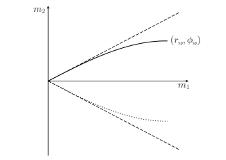
Figure 7: Schematic behaviour of the magnetisation curve (solid line) $(r_{\scriptsize\mbox{sp}},\phi_{\scriptsize\mbox{sp}})$ in the two-dimensional plane that results from the model entropy (43). The angles $-\pi/8$ and $\pi/8$ are indicated by dashed lines. A second solution (dotted line) for the order parameter is obtained by reflecting the spontaneous magnetisation about the $m_{1}$ axis. Application of the rotations in $C_{4v}$ to these two solutions gives the remaining solutions for the order parameter.