Non-Abrikosov Vortex and Topological Knot in Two-gap Superconductor

Abstract

We establish the existence of topologically stable knot in two-gap superconductor whose topology $\pi_{3}(S^{2})$ is fixed by the Chern-Simon index of the electromagnetic potential. We present a helical magnetic vortex solution in Ginzburg-Landau theory of two-gap superconductor which has a non-vanishing condensate at the core, and identify the knot as a twisted magnetic vortex ring made of the helical vortex. We discuss how the knot can be constructed in the recent two-gap $\rm MgB_{2}$ superconductor.

Topological objects, in particular finite energy topological objects have played important role in physics. In condensed matter physics the best known topological object is the Abrikosov vortex in one-gap superconductors (and similar ones in Bose-Einstein condensates and superfluids), which have been the subject of intensive studies. But the advent of two-component BEC and two-gap superconductors bec ; sc has opened a new possibility for us to have far more interesting topological objects in condensed matters ijpap ; prb05 ; ruo ; pra05 ; baba . The purpose of this Letter is two-fold; to present a new type of non-Abrikosov vortex which has a non-vanishing condensate at the core and to establish the existence of a stable knot in Abelian two-gap superconductors. We first construct a new type of non-Abrikosov vortex which has a non-vanishing condensate at the core in Ginzburg-Landau theory of two-gap superconductor, and show that it can be twisted to form a helical magnetic vortex. With this we show that the twisted vortex ring made of the helical magnetic vortex becomes a topological knot whose knot topology $\pi_{3}(S^{2})$ is fixed by the Chern-Simon index of the electromagnetic potential. The knot has two supercurrents, the electromagnetic current around the knot tube which confines the magnetic flux and the neutral current along the knot which generates a net angular momentum which prevents the collapse of the knot, This means that the knot has a dynamical (as well as topological) stability.

There have been two objections against the existence of a stable magnetic vortex ring in Abelian superconductors. First, it is supposed to be unstable due to the tension created by the ring huang . Indeed if one contructs a vortex ring from an Abrikisov vortex, it becomes unstable because of the tension. On the other hand, if we first twist the magnetic vortex making it periodic in $z$-coordinate and then make a vortex ring connecting the periodic ends together, it should become a stable vortex ring. This is because the non-trivial twist of the magnetic field forbids the untwisting of the vortex ring by any smooth deformation of field configuration. The other objection is that the Abelian gauge theory is supposed to have no non-trivial knot topology which alows a stable vortex ring. This again is a common misconception. Actually the theory has a well-defined knot topology $\pi_{3}(S^{2})$ described by the Chern-Simon index of the electromagnetic potential. So a priori there is no reason whatsoever why the Abelian superconductor can not have a topological knot. The real question then is whether the dynamics of the superconductor can actually allow such a knot configuration. In the following we show that indeed a two-gap Abelian superconductor does.

In mean field approximation the Hamiltonian of the Ginzburg-Landau theory of two-gap superconductor could be expressed by baba

$${\cal H}=\displaystyle\frac{\hbar^{2}}{2m_{1}}|(\mbox{\boldmath$\nabla$}+ig\mbox{\boldmath$A$})\tilde{\phi}_{1}|^{2}+\displaystyle\frac{\hbar^{2}}{2m_{2}}|(\mbox{\boldmath$\nabla$}+ig\mbox{\boldmath$A$})\tilde{\phi}_{2}|^{2}$$

$$+\tilde{V}(\tilde{\phi}_{1},\tilde{\phi}_{2})+\displaystyle\frac{1}{2}(\mbox{\boldmath$\nabla$}\times\mbox{\boldmath$A$})^{2},$$ (1)

where $\tilde{V}$ is the effective potential. One can simplify the above Hamiltonian with a proper normalization of $\tilde{\phi}_{1}$ and $\tilde{\phi}_{2}$ to $\phi_{1}=(\hbar/\sqrt{2m_{1}}/)\tilde{\phi}_{1}$ and $(\hbar/\sqrt{2m_{2}})\tilde{\phi}_{2}$,

$${\cal H}=|(\mbox{\boldmath$\nabla$}+ig\mbox{\boldmath$A$})\phi|^{2}+V(\phi)+\displaystyle\frac{1}{2}(\mbox{\boldmath$\nabla$}\times\mbox{\boldmath$A$})^{2},$$ (2)

where $\phi=(\phi_{1},\phi_{2})$ and $V$ is the normalized potential. A most general quartic potential which has the $U(1)\times U(1)$ symmetry is given by

$$V=\displaystyle\frac{\lambda_{11}}{2}|\phi_{1}|^{4}+\lambda_{12}|\phi_{1}|^{2}|\phi_{2}|^{2}+\displaystyle\frac{\lambda_{22}}{2}|\phi_{2}|^{4}$$

$$-\mu_{1}|\phi_{1}|^{2}-\mu_{2}|\phi_{2}|^{2},$$ (3)

where ${\lambda}_{ij}$ are the quartic coupling constants and $\mu_{i}$ are the chemical potentials. But in this paper we will adopt the following potential for simplicity

$$V=\displaystyle\frac{\lambda}{2}\Big{(}(\phi^{\dagger}\phi)-\displaystyle\frac{\mu^{2}}{\lambda}\Big{)}^{2}+\alpha|\phi_{1}|^{2}|\phi_{2}|^{2}.$$ (4)

Notice that when $\alpha=0$, the Hamiltonian (2) has a global $SU(2)$ symmetry as well as the the local $U(1)$ symmetry, so that the $\alpha$-term can be viewed as a symmetry breaking term of $SU(2)$ to $U(1)$. We choose (4) simply because the existence of the topological objects we discuss in this paper is not so sensitive to the detailed form of the potential.

With the above Hamiltonian one may try to obtain a non-Abelian vortex. With

$$\phi=\displaystyle\frac{1}{\sqrt{2}}\rho\xi,~{}~{}~{}~{}~{}{\xi}^{\dagger}\xi=1,~{}~{}~{}~{}~{}\hat{n}=\xi^{\dagger}\vec{\sigma}\xi,$$

$$C_{\mu}=\displaystyle\frac{2i}{g}\xi^{\dagger}\partial_{\mu}\xi,~{}~{}~{}~{}~{}\rho_{0}=\displaystyle\frac{2\mu^{2}}{\lambda},$$ (5)

we have the following equations of motion ijpap

$$\partial^{2}\rho-\Big{(}\displaystyle\frac{1}{4}(\partial_{\mu}\hat{n})^{2}+g^{2}(A_{\mu}-\displaystyle\frac{1}{2}C_{\mu})^{2}\Big{)}\rho$$

$$=\displaystyle\frac{\lambda}{2}(\rho^{2}-\rho_{0}^{2})\rho+\alpha\rho^{3}\xi_{1}^{*}\xi_{1}\xi_{2}^{*}\xi_{2},$$

$$\hat{n}\times\partial^{2}\hat{n}+2\displaystyle\frac{\partial_{\mu}\rho}{\rho}\hat{n}\times\partial_{\mu}\hat{n}-\displaystyle\frac{2}{g\rho^{2}}\partial_{\mu}F_{\mu\nu}\partial_{\nu}\hat{n}$$

$$=\displaystyle\frac{\alpha}{2}(\hat{k}\cdot\hat{n})\rho^{2}\hat{k}\times\hat{n},$$

$$\partial_{\mu}F_{\mu\nu}=g^{2}\rho^{2}(A_{\mu}-\displaystyle\frac{1}{2}C_{\mu}),$$ (6)

where $\vec{\sigma}$ is the Pauli matrix and $\hat{k}=(0,0,1)$. Notice that it has the vacuum at $\rho=\rho_{0}$, and $\xi=(1,0)$ or $\xi=(0,1)$.

The equation allows two conserved currents, the electromagnetic current $j_{\mu}$ and the neutral current $k_{\mu}$,

$$j_{\mu}=g^{2}\rho^{2}(A_{\mu}-\displaystyle\frac{1}{2}C_{\mu})$$

$$k_{\mu}=g^{2}\rho^{2}\Big{[}A_{\mu}\big{(}\xi_{1}^{*}\xi_{1}-\xi_{2}^{*}\xi_{2}\big{)}+\displaystyle\frac{i}{g}\big{(}\partial_{\mu}\xi_{1}^{*}\xi_{1}$$

$$+\xi_{2}^{*}\partial_{\mu}\xi_{2}\big{)}\Big{]},$$ (7)

which are nothing but the Noether currents of the $U(1)\times U(1)$ symmetry of the Hamiltonian (2). Indeed they are the sum and difference of two electromagnetic currents of $\phi_{1}$ and $\phi_{2}$

$$j_{\mu}=j^{(1)}_{\mu}+j^{(2)}_{\mu},~{}~{}~{}~{}~{}k_{\mu}=j^{(1)}_{\mu}-j^{(2)}_{\mu}.$$ (8)

Clearly the conservation of $j_{\mu}$ follows from the last equation of (6). But the conservation of $k_{\mu}$ comes from the second equation of (6), which (together with the last equation) tells the existence of a partially conserved $SU(2)$ current $\vec{j}_{\mu}$,

$$\vec{j}_{\mu}=g\rho^{2}\Big{(}\frac{1}{2}\vec{n}\times\partial_{\mu}\vec{n}-g(A_{\mu}-\frac{1}{2}C_{\mu})\vec{n}\Big{)}.$$ (9)

This $SU(2)$ current is exactly conserved when $\alpha=0$. But notice that $k_{\mu}=\hat{k}\cdot\vec{j}_{\mu}$. This assures the conservation of $k_{\mu}$ even when $\alpha\neq 0$. It is interesting to notice that $j_{\mu}$ and $k_{\mu}$ are precisely the $\hat{n}$ and $\hat{k}$ components of $\vec{j}_{\mu}$.

To obtain the desired knot we construct a helical magnetic vortex first ijpap . Let $(\varrho,\varphi,z)$ be the cylindrical coodinates and let

$$\rho=\rho(\varrho),~{}~{}~{}~{}~{}\xi=\Bigg{(}\matrix{\cos\displaystyle\frac{f(\varrho)}{2}\exp(-in\varphi)\cr\sin\displaystyle\frac{f(\varrho)}{2}\exp(imkz)}\Bigg{)},$$

$$A_{\mu}=\displaystyle\frac{1}{g}\Big{(}nA_{1}(\varrho)\partial_{\mu}\varphi+mkA_{2}(\varrho)\partial_{\mu}z\Big{)},$$ (10)

and find

$$\hat{n}=\Bigg{(}\matrix{\sin{f(\varrho)}\cos{(n\varphi+mkz)}\cr\sin{f(\varrho)}\sin{(n\varphi+mkz)}\cr\cos{f(\varrho)}}\Bigg{)},$$

$$C_{\mu}=\displaystyle\frac{\cos{f(\varrho)}+1}{g}n\partial_{\mu}\varphi+\displaystyle\frac{\cos{f(\varrho)}-1}{g}mk\partial_{\mu}z,$$

$$j_{\mu}=g\rho^{2}\Big{(}n\big{(}A_{1}-\displaystyle\frac{\cos{f}+1}{2}\big{)}\partial_{\mu}\varphi$$

$$+mk\big{(}A_{2}-\displaystyle\frac{\cos{f}-1}{2}\big{)}\partial_{\mu}z\Big{)},$$

$$k_{\mu}=g\rho^{2}\Big{(}n\big{(}A_{1}\cos{f}-\displaystyle\frac{\cos{f}+1}{2}\big{)}\partial_{\mu}\varphi$$

$$+mk\big{(}A_{2}\cos{f}+\displaystyle\frac{\cos{f}-1}{2}\big{)}\partial_{\mu}z\Big{)}.$$ (11)

With this (6) becomes

$$\ddot{\rho}+\displaystyle\frac{1}{\varrho}\dot{\rho}-\Big{[}\displaystyle\frac{1}{4}\Big{(}\dot{f}^{2}+\big{(}\displaystyle\frac{n^{2}}{\varrho^{2}}+m^{2}k^{2}\big{)}\sin^{2}{f}\Big{)}$$

$$+\displaystyle\frac{n^{2}}{\varrho^{2}}\Big{(}A_{1}-\displaystyle\frac{\cos{f}+1}{2}\Big{)}^{2}+m^{2}k^{2}\Big{(}A_{2}-\displaystyle\frac{\cos{f}+1}{2}\Big{)}^{2}\Big{]}\rho$$

$$=\displaystyle\frac{\lambda}{2}(\rho^{2}-\rho_{0}^{2})\rho+\displaystyle\frac{\alpha}{4}\rho^{3}\sin^{2}f,$$

$$\ddot{f}+\big{(}\displaystyle\frac{1}{\varrho}+2\displaystyle\frac{\dot{\rho}}{\rho}\big{)}\dot{f}-2\Big{(}\displaystyle\frac{n^{2}}{\varrho^{2}}\big{(}A_{1}-\displaystyle\frac{1}{2}\big{)}$$

$$+m^{2}k^{2}\big{(}A_{2}+\displaystyle\frac{1}{2}\big{)}\Big{)}\sin{f}=\displaystyle\frac{\alpha}{4}\rho^{2}\sin 2f,$$

$$\ddot{A}_{1}-\displaystyle\frac{1}{\varrho}\dot{A}_{1}-g^{2}\rho^{2}\Big{(}A_{1}-\displaystyle\frac{\cos{f}+1}{2}\Big{)}=0,$$

$$\ddot{A}_{2}+\displaystyle\frac{1}{\varrho}\dot{A}_{2}-g^{2}\rho^{2}\Big{(}A_{2}-\displaystyle\frac{\cos{f}-1}{2}\Big{)}=0.$$ (12)

Now, we impose the following boundary condition for the non-Abelian vortex,

$$\dot{\rho}(0)=0,~{}~{}~{}\rho(\infty)=\rho_{0},~{}~{}~{}f(0)=\pi,~{}~{}~{}f(\infty)=0,$$

$$A_{1}(0)=0,~{}~{}~{}A_{1}(\infty)=1,$$

$$\dot{A}_{2}(0)=0,~{}~{}~{}A_{2}(\infty)=0.$$ (13)

This need some explanation. First, notice that here we have $\dot{\rho}(0)=0$, not $\rho(0)=0$. This would have been unacceptable in one-gap superconductor because this would create a singularity at the core of the vortex. But with the ansatz (10) the boundary condition allows a smooth vortex in two-gap superconductor. Secondly, we have $\dot{A}_{2}(0)=0$ in stead of a condition on $A_{2}(0)$. It turns out that this is the correct way to obtain a smooth solution. Indeed we find that $A_{2}(0)$ is determined by $k$.

Figure 1: The helical vortex (solid line) with $m=n=1$ and the straight vortex (dotted line) $m=0$ and $n=1$ in two-gap superconductor. Here we have put $g=1,~{}\lambda=2$, $k=0.1~{}\rho_{0}$, $~{}\alpha=0.01$, and $\varrho$ is in the unit of $1/\rho_{0}$. Notice that the straight vortex has no $A_{2}$.

With the boundary condition we can integrate (12) and obtain the non-Abelian vortex solution of the two-gap superconductor which is shown in Fig.1. Notice that we have plotted $\rho_{1}=\rho\cos f/2$ and $\rho_{2}=\rho\sin f/2$ which represent the density of $\phi_{1}$ and $\phi_{2}$, in stead of $\rho$ and $f$, in the figure. There are three points that should be emphasized here. First, the doublet $\phi$ starts from the second component at the core, but the first component takes over completely at the infinity. This is due to the boundary condition $f(0)=\pi$ and $f(\infty)=0$, which assures that our solution describes a new type of non-Abrikosov vortex which has a non-vanishing condensate at the core ijpap . Secondly the electromagnetic current $j_{\mu}$ of the vortex is helical, so that it creates a helical magnetic flux which has a quantized flux $\Phi_{\hat{z}}=2\pi n/g$ around the $z$-axis as well as a (fractionally) quantized flux $\Phi_{\hat{\varphi}}=-2\pi mA_{2}(0)/g$ along the $z$-axis. And obviously the two magnetic fluxes are linked together. But it creates a net current $i_{\hat{\varphi}}$ only around the $z$-axis, with $i_{\hat{z}}=i^{(1)}_{\hat{z}}+i^{(2)}_{\hat{z}}=0$. Finally the vortex has another (neutral) helical $k_{\mu}$, which has a net current $k_{\hat{z}}$ along the $z$-axis (as well as $k_{\hat{\varphi}}$ around the vortex). Notice that $k_{\hat{z}}=i^{(1)}_{\hat{z}}-i^{(2)}_{\hat{z}}=2i^{(1)}_{\hat{z}}$. This is because the two electromagnetic currents $i^{(1)}_{\hat{z}}$ and $i^{(2)}_{\hat{z}}$ of $\phi_{1}$ and $\phi_{2}$ are equal but flow oppositely, which generates a nonvanishing $k_{\hat{z}}$. This is why we call $k_{\mu}$ a neutral current. In this sense the vortex can be viewed as superconducting, even though the net electromagnetic current along the knot is zero. The two helical supercurrents $j_{\mu}$ and $k_{\mu}$ are plotted in Fig. 2.

Figure 2: The helical supercurrents with $m=n=1$ in two-gap superconductor. Here we have put $g=1,~{}\lambda=2$, $k=0.1~{}\rho_{0}$, $~{}\alpha=0.01$, and $\varrho$ is in the unit of $1/\rho_{0}$.

Of course, the helical magnetic vortex has only a heuristic value, because it will be untwisted unless the periodicity condition is enforced by hand. But if we make a vortex ring by smoothly bending and connecting two periodic ends, the periodicity condition is naturally enforced. And the twisted magnetic vortex ring becomes a topological knot ijpap . There are two ways to describe the knot topology. First, the doublet $\xi$ (in the vortex ring) acquires a non-trivial topology $\pi_{3}(S^{2})$ which provides the knot quantum number,

$$Q=-\displaystyle\frac{1}{4\pi^{2}}\int\epsilon_{ijk}\xi^{\dagger}\partial_{i}\xi(\partial_{j}\xi^{\dagger}\partial_{k}\xi)d^{3}x$$

$$=\displaystyle\frac{g^{2}}{32\pi^{2}}\int\epsilon_{ijk}C_{i}(\partial_{j}C_{k}-\partial_{k}C_{j})d^{3}x=mn.$$ (14)

This is nothing but the Chern-Simon index of the potential $C_{\mu}$. Perhaps more importantly, the knot topology can also be described by the Chern-Simon index of the electromagnetic potential $A_{\mu}$. Indeed we have

$$Q=\displaystyle\frac{g^{2}}{8\pi^{2}}\int\epsilon_{ijk}A_{i}F_{jk}d^{3}x=mn,$$ (15)

which describes the twisted knot topology of the real (physical) magnetic flux. It describes the linking number of two quantized magnetic fluxes $\Phi_{\hat{z}}$ and $\Phi_{\hat{\varphi}}$. Obviously two flux rings linked together can not be separated by any continuous deformation of the field configuration. This provides the topological stability of the knot.

Furthermore the topological stability is backed up by a dynamical stability. This is because the knot is made of two quantized magnetic fluxes linked together. And the flux trapped inside of the knot ring can not be squeezed out, and provides a repulsive force against the collapse of the knot. This makes the knot dynamically stable. Another way to understand this dynamical stability is to notice that the neutral supercurrent $k_{\hat{z}}$ of the helical vortex becomes a supercurrent along the knot, which generates a net angular momentum around the knot. And this provides the centrifugal repulsive force preventing the knot to collapse. This makes the knot dynamically stable. We can find the energy profile of the twisted magnetic vortex ring numerically. Minimizing the energy we obtain the energy profile of the knot shown in Fig. 3.

Clearly the dynamical stability of the knot comes from the helical structure of the vortex. But this helical structure is precisely what provides the knot topology to the vortex ring. The nontrivial topology expresses itself in the form of the helical magnetic flux which provides the dynamical stability of the knot. Conversely the helical magnetic flux assures the existence of the knot topology which guarantees the topological stability of the knot. It is this remarkable interplay between dynamics and topology which assures the existence of the stable superconducting knot in two-gap superconductor.

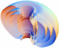
Figure 3: (Color online). The energy profile of superconducting knot with $m=n=1$. Here we have put $g=1,~{}\lambda=2$, $k=0.1~{}\rho_{0}$, $~{}\alpha=0.01$.

We close with the following remarks:
1. The existence of a knot in two-gap superconductor has been conjectured before ijpap ; baba . In fact, similar knots have been asserted to exist almost everywhere in physics, in atomic physics in two-component Bose-Einstein condensates ijpap ; ruo ; pra05 , in nuclear physics in Skyrme theory fadd ; prl01 , in high energy physics in QCD plb05 . In this paper we have provided a concrete evidence for the existence of a stable knot in two-gap superconductor, which can be interpreted as a twisted magnetic vortex ring.
2. In this Letter we have concentrated on the Abelian gauge theory of two-gap superconductor, which is made of two condensates of same charge. But we emphasize that a similar knot should also exist in the non-Abelian gauge theory of two-gap superconductor which describes two condensates of opposite charge prb05 . This is because two theories are mathematically identical to each other. This implies that such a knot can also exist in the liquid metallic hydrogen (LMH), because it can also be viewed as a non-Abelian two-gap superconductor made of opposite charge (the proton pairs and the electron pairs) ash .
3. One should try to construct the topological knot experimentally in two-gap superconductors. But before one does that, one must first confirm the existence of the non-Abrikosov vortex which has a non-vanishing condensate (the second component) at the core. This is very important because this will prove the existence of a new type of magnetic vortex in two-gap superconductor. With this confirmation one may try to construct the helical vortex and the knot. With some experimental ingenuity one should be able to construct these topological objects in $\rm MgB_{2}$ or $\rm LMH$.

As we have remarked there is a wide class of realistic potentials which allows similar non-Abrikosov vortex and topological knot. The detailed discussion on the subject and its applications in the presence of a more general potential which includes the Josephson interaction will be discussed separately cho1 .

ACKNOWLEDGEMENT

The work is supported in part by the ABRL Program of Korea Science and Enginnering Foundation (Grant R14-2003-012-01002-0), and by the BK21 Project of the Ministry of Education.

References

- (1) C. Myatt at al., Phys. Rev. Lett. 78, 586 (1997); D. Stamper-Kurn, at al., Phys. Rev. Lett. 80, 2027 (1998).
- (2) J. Nagamatsu et al., Nature 410, 63 (2001); S. L. Bud’ko et al., Phys. Rev. Lett. 86, 1877 (2001); C. U. Jung et al., Appl. Phys. Lett. 78, 4157 (2001).
- (3) Y. M. Cho, cond-mat/012325; Int. J. Pure Appl. Phys. 1, 246 (2005).
- (4) Y. M. Cho, cond-mat/012492; Phys. Rev. B72, 212516 (2005).
- (5) U. Al Khawaja and H. Stoof, Nature 411, 918 (2001); C. Savage and J. Ruostekoski, Phys. Rev. Lett. 91, 010403 (2003).
- (6) Y. M. Cho, H. J. Khim, and Pengming Zhang, Phys. Rev. A72, 063603 (2005).
- (7) E. Babaev, Phys. Rev. Lett. 89, 067001 (2002); E. Babaev, L. Faddeev, and A. Niemi, Phys. Rev. B65, 100512 (2002).
- (8) K. Huang and R. Tipton, Phys. Rev. D23, 3050 (1981).
- (9) L. Faddeev and A. Niemi, Nature 387, 58 (1997); R. Battye and P. Sutcliffe, Phys. Rev. Lett. 81, 4798 (1998).
- (10) Y. M. Cho, Phys. Rev. Lett. 87, 252001 (2001); Phys. Lett. B603, 88 (2004).
- (11) Y. M. Cho, Phys. Lett. B616, 101 (2005).
- (12) N. Ashcroft, Phys. Rev. Lett. 92, 187002 (2004); E. Babaev, A. Sudbe, and N. Ashcroft, Nature 431, 666 (2004).
- (13) Y. M. Cho, and Pengming Zhang, to be published.