Impact of weak localization in the time domain

Abstract

We find a renormalized “time-dependent diffusion coefficient”, $D(t)$, for pulsed excitation of a nominally diffusive sample by solving the Bethe-Salpeter equation with recurrent scattering. We observe a crossover in dynamics in the transformation from a quasi-1D to a slab geometry implemented by varying the ratio of the radius, $R$, of the cylindrical sample with reflecting walls and the sample length, $L$. Immediately after the peak of the transmitted pulse, $D(t)$ falls linearly with a nonuniversal slope that approaches an asymptotic value for $R/L\gg 1$. The value of $D(t)$ extrapolated to $t=0$ depends only upon the dimensionless conductance $g$ for $R/L\ll 1$ and only upon $k\ell_{0}$ for $R/L\gg 1$, where $k$ is the wave vector and $\ell_{0}$ is the bare mean free path.

Weak localization (WL) of electronic and classical waves arises from the interference of counterpropagating partial waves in closed loops. Its impact upon electronic conductance Mesobook has been widely studied using steady-state methods such as magnetoresistance Bergmann , and can be directly visualized as enhanced retroreflection of light from random samples CBS . Partial waves with trajectories over a wide range of lengths contribute to these phenomena. It is, however, of great interest to investigate the variation of WL upon pathlength Altshuler ; Berkovits90 ; Weaver94 ; Mirlin00 ; Chabanov02 since the impact of WL presumably increases with pathlength. Though it has not been practical to isolate paths of specific lengths in studies of electronic conductance, this can be accomplished for classical waves in time-resolved measurements of pulsed transmission through random media Chabanov02 ; McCall87 ; GenDrake89 ; Alfano90 ; Lagendijk97 ; Zang99 . Time-resolved transmission measurements McCall87 ; GenDrake89 have generally been consistent with diffusion theory, which predicts a simple exponential decay of the average transmission following an initial rise, with the decay rate due to leakage from the sample of $1/t_{D}=\pi^{2}D_{0}/(L+2z_{0})^{2}$, where $t_{D}$ is the diffusion time, $D_{0}$ is the diffusion coefficient, $L$ is the sample thickness, and $z_{0}$ is the extrapolation length. Recently, however, Chabanov el al. Chabanov02 observed nonexponential decay of pulsed microwave transmission in a quasi-1D sample which they characterized by a “time-dependent diffusion coefficient”, $D(t)$. The decrease in the decay rate with time was compared to the leading correction term in a supermatrix model calculation by Mirlin Mirlin00 of the tail of the electron survival probability. In the case of the orthogonal ensemble, it can be expressed in term of the renormalization of a “time-dependent diffusion coefficient”, $D(t)/D_{0}=1-(2/\pi^{2}gt_{D})t$, where $g$ is the dimensionless conductance. A linear decay of $D(t)$ was found in microwave experiments; however, $D(t)$ did not extrapolate to the bare diffusion coefficient at $t=0$ and the scaling behavior of the slope of $D(t)$ did not agree with the above expression. Nonexponential decay of pulsed transmission has also been reported recently in numerical simulations in 2D Haney03 and in a self-consistent diffusion theory, which includes recurrent scattering Bart03 . For times much larger than the Heisenberg time, $t_{H}=gt_{D}$, it has been predicted that the decay of the electron survival probability follows a log-normal behavior due to the presence of prelocalized states Altshuler . These long-lived states might be associated with rare configurations of disorder in the medium Apalkov02 .

In this Letter, we solve the Bethe-Salpeter equation with recurrent scattering included in a self-consistent manner that satisfies the Ward Identity Kirkpatrick85 to obtain the average time-dependent intensity transmitted through a random sample following pulsed excitation. The sample is cylindrical with reflecting walls. By changing the ratio of the longitudinal dimension $L$ and the radius $R$, a smooth transition can be made between two key experimental geometries: a quasi-1D geometry with $L\gg R$, which is commonly employed in microwave experiments, and a slab with $L\ll R$, which is the typical optical geometry. For the quasi-1D geometry, we find $D(t)/D_{0}=A-(2B/\pi^{2}gt_{D})t$ for $t\ll t_{H}$. The constant part, $A$, is universal, depending only on $g$, while $B$ is nonuniversal and depends upon $L/\ell_{0}$, where $\ell_{0}$ is the bare mean free path, as well as upon $g$. In the limit $g\gg 1$ and $L/\ell_{0}\gg 1$, our results coincide with supersymmetry calculations by Mirlin Mirlin00 . For intermediate values of $g$, $g\geq 5$, our results are in agreement with experiment Chabanov02 . For the slab geometry, $D$ approaches a nearly constant renormalized value, being equal to $D_{0}(1-1.03/(k\ell_{0})^{2})$ in the limit $L/\ell_{0}\gg 1$. This is close to the result of WL theory for a bulk system.

We consider a scalar wave incident on the front surface of the random sample at $z=0$. We assume that the medium possesses neither absorption nor gain and that scattering is isotropic. The time evolution of intensity within the sample is obtained from the Fourier transform of the frequency correlation function $C_{\Omega}(\omega,\mathbf{r})=\langle\phi_{\Omega^{+}}(\mathbf{r})\,\phi^{*}_{\Omega^{-}}(\mathbf{r})\rangle$, where $\Omega^{\pm}=\Omega\pm\omega/2$, $\Omega$ is the wave frequency, $\omega$ is the frequency shift, and $\phi_{\Omega}(\mathbf{r})$ is the wavefunction or field inside the sample Zang99 ; GenDrake89 . The function $C_{\Omega}(\omega,\mathbf{r})$ is obtained from the space-frequency correlation function $C_{\Omega}(\omega,\mathbf{r},\mathbf{r}^{\prime})=\langle\phi_{\Omega^{+}}(\mathbf{r})\,\phi^{*}_{\Omega^{-}}(\mathbf{r}^{\prime})\rangle$, which satisfies the Bethe-Salpeter equation,

$$C_{\Omega}(\omega,\mathbf{r},\mathbf{r}^{\prime})\!\!\! = \!\!\!\langle\phi_{\Omega^{+}}(\mathbf{r})\rangle\,\langle\phi^{*}_{\Omega^{-}}(\mathbf{r}^{\prime})\rangle$$

$$+\int\!\!\!\! d\mathbf{r}_{1} \!\!\!d\mathbf{r}_{2}\,d\mathbf{r}_{3}\,d\mathbf{r}_{4}\langle G_{\Omega^{+}}(\mathbf{r},\mathbf{r}_{1})\rangle\langle\,G_{\Omega^{-}}(\mathbf{r}^{\prime},\mathbf{r}_{3})\rangle\,$$ (1)

$$\times \!\!\!U_{\Omega}(\omega\,;\mathbf{r}_{1},\mathbf{r}_{2}\,;\mathbf{r}_{3},\mathbf{r}_{4})\,C_{\Omega}(\omega,\mathbf{r}_{2},\mathbf{r}_{4})\,,$$

where $\langle\phi_{\Omega}(\mathbf{r})\rangle$ represents the coherent source inside the sample and $\langle G_{\Omega}(\mathbf{r},\mathbf{r}_{1})\rangle=-{\exp(iK|\mathbf{r}-\mathbf{r}_{1}|)\over 4\pi|\mathbf{r}-\mathbf{r}_{1}|}$ is the ensemble-averaged Green’s function. Here $K=k+{i\over 2\ell}$, where $k={\Omega\over v}$, $v$ is the wave speed, $\ell$ is the scattering mean free path determined from the imaginary part of the self-energy of $\langle G\rangle$. $\ell_{0}$ is determined from the single-scattering diagram only. The vertex function $U_{\Omega}$ in Eq. (1) represents the sum of all irreducible vertices. Here we approximate $U_{\Omega}$ as

$$U_{\Omega}(\omega;\mathbf{r}_{1},\mathbf{r}_{2};\mathbf{r}_{3},\mathbf{r}_{4})=$$ (2)

$${4\pi\over\ell_{0}}[1+\delta(\omega,k)]\,\delta(\mathbf{r}_{1}-\mathbf{r}_{2})\,\delta(\mathbf{r}_{1}-\mathbf{r}_{3})\,\delta(\mathbf{r}_{1}-\mathbf{r}_{4}).$$

The first term, proportional to $4\pi/\ell_{0}$, generates all self-avoiding multiple-scattering diagrams, which produce the diffusion result when $L\gg\ell_{0}$ Lagendijk88 , whereas the factor $\delta(\omega,k)$ in the second term represents the WL contribution to $U_{\Omega}$. The presence of the second term in the vertex function renormalizes the mean free path, giving $\ell(\omega,k)=\ell_{0}/[1+\delta(\omega,k)]$. The Ward Identity, which enforces flux conservation, requires that the same $\ell(\omega,k)$ should appear in $\langle G\rangle$ of Eq. (1). Here, we assume that the system is far from the localization threshold and that the renormalized mean free path is scale independent. In a bulk system, $\delta(\omega,k)$ can be obtained from the renormalized frequency-dependent diffusion coefficient Kirkpatrick85 ,

$$\frac{1}{D(\omega,k)}={\frac{1}{D_{0}}}[1+\frac{2\pi v}{k^{2}}\tilde{G}(\mathbf{r},\mathbf{r};\omega)],$$ (3)

where $D(\omega,k)=v\ell(\omega,k)/3$, and $\tilde{G}$ is the Green’s function for the diffusion equation and reflects the return probability. Here, we solve for $\tilde{G}$ by using the boundary conditions of a reflecting tube. After taking the spatial average, we find

$$\delta(\omega,k)=\delta_{1}(\omega,k)+\delta_{2}(\omega,k),$$ (4)

with

$$\delta_{1}(\omega,k)=\frac{v}{2N\tilde{L}}\sum^{n_{c}}_{n=1}\frac{1}{-i\omega+D_{0}q_{n}^{2}}$$ (5)

and

$$\delta_{2}(\omega,k)=\frac{3}{2k^{2}l_{0}\tilde{L}}\sum^{n_{c}}_{n=1}\ln\!\left(\frac{-i\omega+D_{0}(q_{n}^{2}+\alpha^{2}/l_{0}^{2})}{-i\omega+D_{0}(q_{n}^{2}+\pi^{2}/R^{2})}\right),$$ (6)

where $N=(kR)^{2}/4$ is the number of transverse modes, $q_{n}=n\pi/\tilde{L}$, $n_{c}=\alpha\tilde{L}/\pi l_{0}$, and $\tilde{L}=L+2z_{0}$ with $z_{0}=0.71\ell_{0}$ Morse . In the above equations, $\alpha/\ell_{0}$ denotes the upper momentum cutoff, $q_{c}$, and is chosen as $1/\ell_{0}$ in our calculations unless specified otherwise. The $\delta_{1}$ term arises from diffusive modes which are uniform in the transverse directions, i.e., $\vec{q}_{\perp}=0$. When $L/\ell_{0}$ is large, the static limit of this term becomes $\delta_{1}(\omega=0)=1/3g$, where $g=4N\ell_{0}/3\tilde{L}$. This term is responsible for the linear decrease of the decay rate in the transmitted intensity $\langle I(t)\rangle$. The $\delta_{2}$ term represents the contribution from other transverse modes below $\vec{q}_{\perp,c}$. This term becomes important only when $R\gg\ell_{0}$ and is responsible for the renormalization of diffusion constant in the limit of a slab geometry. In our calculation, we replace $D_{0}$ in Eqs. (5) and (6) by $v\ell(\omega,k)/3$ and solve for $\delta(\omega,k)$ in a self-consistent manner.

For simplicity of calculation, we assume both the excitation intensity and the scattered intensity are uniform in the transverse cross-section of the tube. Eq. (1) can now be written as Zang99

$$C_{\Omega}(\omega\!\!\!\!\! \!\!\!\!z)=\exp\!\left({i\omega z\over v}-{z\over\ell_{0}}\right)$$ , (7)

$$+ \!\!{1+\delta(k,\omega)\over 4\pi\ell_{0}}\int_{0}^{L}\!\!dz^{\prime}H(\omega,z-z^{\prime})\,C_{\Omega}(\omega,z^{\prime})\,,$$

where

$$H(\omega,z-z^{\prime})=\pi\!\int\!\!d\rho^{2}{\exp\!\left[\left({i\omega\over v}-{[1+\delta(\omega,k)]\over\ell_{0}}\right)\!\sqrt{\rho^{2}+(z-z^{\prime})^{2}}\right]\over\rho^{2}+(z-z^{\prime})^{2}}\,.$$ (8)

Eq. (7) is solved numerically for $C_{\Omega}(\omega,L)$. Its Fourier transform gives $\langle I(t)\rangle$, from which we can calculate the renormalized “time-dependent diffusion coefficient”, $D(t)/D_{0}=-t_{D}\,d\ln\langle I(t)\rangle/dt$, for $t>t_{D}$ Chabanov02 .

We first consider a quasi-1D geometry with $L\gg R\simeq\ell_{0}$. In this case, since $\delta_{2}$ is nonzero only when $R>\pi\ell_{0}/\alpha$, we can set $\delta_{2}=0$. For the case of $N=800$, $D(t)/D_{0}$ is plotted in Fig. 1 as a function of the dimensionless time, $t^{\prime\prime}\equiv 2t/\pi^{2}gt_{D}$, for $L/\ell_{0}$=20, 40, and 80. Also plotted in Fig. 1 (dotted line) is Mirlin’s analytical result Mirlin00 , $D(t^{\prime\prime})/D_{0}=1-t^{\prime\prime}$. The decay rate of $D(t^{\prime\prime})/D_{0}$ appears to decrease with increasing $L/\ell_{0}$ and is always smaller than the analytical result. If we fit the linear region to $D(t^{\prime\prime})/D_{0}=A-Bt^{\prime\prime}$, the intercept $A$ is found to decrease with increasing $L/\ell_{0}$. These observations are consistent with recent microwave experiments Chabanov02 . In order to understand the behavior of $A$ and $B$, we have carried out a systematic study by varying $L/\ell_{0}$ and $N$. The results for $A$ are shown in Fig. 2, where $A$ is plotted as a function of $g$ for $L/\ell_{0}$=10, 20, and 40. All the data points can be well fit by a single curve, $A=1.00-0.27/g-0.17/g^{2}$, indicating that $A$ is a function only of $g$. In the limit of large $g$, we recover Mirlin’s result, $A=1$. It is interesting to note that the above relation gives, $\beta=d\ln\!A/d\ln\!\tilde{L}=-(0.27/g+0.34/g^{2})/A$, which corresponds to the exponent of the local scaling relation, $A\propto\tilde{L}^{\beta}$. If we use the value in the microwave experiments Chabanov02 of $g=5.5$, we find $\beta=-0.06$, which is in good agreement with the measured value of $-0.05$.

Figure 1: $D(t^{\prime\prime})/D_{0}$ plotted as a function of the dimensionless time, $t^{\prime\prime}\equiv 2t/\pi^{2}gt_{D}$, for quasi-1D samples with $N=800$. The dotted line is the analytical result of Ref. [7], $1-t^{\prime\prime}$.

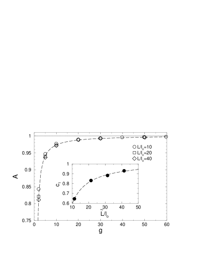
Figure 2: The parameter $A$ obtained from the fit of $D(t^{\prime\prime})/D_{0}$ with $A-Bt^{\prime\prime}$ is plotted as a function of $g$ for quasi-1D samples. The dashed curve is $A=1.00-0.27/g-0.17/g^{2}$. In the inset: $c_{1}$ versus $\tilde{L}/\ell_{0}$; the dashed curve is $c_{1}=1.03-4.42\ell_{0}/\tilde{L}$.

Figure 3: The parameter $B$ obtained from the fit of $D(t^{\prime\prime})/D_{0}$ with $A-Bt^{\prime\prime}$ is plotted as a function of $g$ for quasi-1D samples. The dashed curves are the fit of $B$ with $B=B_{0}+B_{1}/g+B_{2}/g^{2}$, where $B_{i}$ are constant. In the inset: $B_{0}$ versus $(L/\ell_{0})^{-1}$; the dashed line represents a linear fit.

Figure 4: $D(t^{\prime\prime})/D_{0}$ plotted as a function of $t^{\prime}=t/t_{D}$ for three samples studied in Ref. [8], with $N=68$, $L/\ell_{0}=6.4$ (Sample A), 9.5 (Sample B), and 19.2 (Sample C), and $D_{0}=41.5$ cm²/ns. The theoretical results for the corresponding samples are shown as solid curves.

Figure 5: The parameter $A$ obtained from the fit of $D(t^{\prime\prime})/D_{0}$ with $A-Bt^{\prime\prime}$ is plotted as a function of $g$ for $L/\ell_{0}=20$ and different radii $R/\ell_{0}$. The dashed curves are the fit of $A$ with $A=A_{0}+A_{1}/g+A_{2}/g^{2}$, where $A_{i}$ are constant. In the inset: $A$ versus $2R/L$ for $k\ell_{0}=4$ (A), 6 (B), 8 (C), and 12 (D).

The corresponding results for $B$ are shown in Fig. 3. Unlike $A$, $B$ depends not only on $g$ but also on $L/\ell_{0}$. For each $L/\ell_{0}$, we fit $B$ with $B_{0}+B_{1}/g+B_{2}/g^{2}$, where $B_{i}=B_{i}(L/\ell_{0})$. The values of $B_{0}$ are found to be linear in $(\tilde{L}/\ell_{0})^{-1}$, as shown in the inset. In the limit of large $L/\ell_{0}$, $B_{0}$ approaches the Mirlin’s result of $B=1$. Thus, our calculations indicate that Mirlin’s result is valid only when both $g$ and $L/\ell_{0}$ are sufficiently large. In Fig. 4, we compare our theory with microwave measurements Chabanov02 for $N=68$ and $L/\ell_{0}=6.4$ (Sample A), $9.5$ (Sample B), and $19.2$ (Sample C), corresponding to $\ell_{0}=9.5$ cm. The best fit is found for $\alpha=0.5$, and good agreement is found for Samples A and B. For Sample C, for which $g=3$, however, our theory predicts a smaller decay rate, reflecting the important role of localization effects, which are not included here.

We next consider the crossover from a quasi-1D to a slab geometry, as $R/L$ increases. When $2R/L$ is sufficiently large, the $\delta_{1}$ term falls leading to a slope of $D(t)$ with a magnitude which decreases as $1/g\propto 1/R^{2}$. In the limit of large $R/L$, the function $D(t)$ approaches a nearly constant value, $\tilde{D}$, which is determined by the $\delta_{2}$ term. Thus, we focus our discussion on $A$. In Fig. 5, we present $A$ as a function of $g$ for different values of $R/\ell_{0}$ for $L/\ell_{0}=20$. These results suggest, $A=1-c_{0}(L,R)/g$. From the fit (dashed lines) to the data, we find that $c_{0}(L,R)$ is proportional to $R^{2}$ when $2R>L$, suggesting $A=1-c_{1}(L)/(k\ell_{0})^{2}$. This can also be seen in the inset of Fig. 5, where $A$ is replotted as a function of $2R/L$ for different values of $k\ell_{0}$. It is seen that $A$ approaches a constant value when $2R>L$ for each value of $k\ell_{0}$. In order to find the behavior of $c_{1}(L)$, we repeat the calculation for $L/\ell_{0}=10$, 30 and 40. The results are plotted in the inset of Fig. 2. The fitting of these data suggests, $c_{1}=1.03-4.42\ell_{0}/\tilde{L}$ (dashed line), which is the behavior of the renormalized diffusion coefficient $\tilde{D}$ in a slab. Thus $\tilde{D}$ decreases with increasing $L$, which is due to the presence of longer recurrent scattering paths in a thicker sample. This behavior is different from that found in thin samples in optical measurements when $L/\ell_{0}<6$ Lagendijk97 . It is interesting to note that when $L/\ell_{0}\gg 1$, our result $\tilde{D}/D_{0}\simeq 1-1.03/(k\ell_{0})^{2}$ is close to the static result of Eq. (3) in the bulk for $\alpha=1$, i.e., $1-3\alpha/\pi(k\ell_{0})^{2}$.

In conclusion, we have solved the Bethe-Salpeter equation with recurrent scattering to obtain WL in the time domain. Following peak of the transmitted pulse, the “time-dependent diffusion coefficient” $D(t)$ falls nearly linearly. We find the extrapolated value of $D(t)$ at $t=0$ and the slope of $D(t)$ for samples with different scattering strengths, as the aspect ratio of the sample is changed, transforming the sample geometry from a quasi-1D to a slab. From this prospective, WL in steady-state measurements can be understood in terms of the increasing impact of WL associated with trajectories of increasing length.

Discussions with P. Sheng are gratefully acknowledged. This research is supported by Hong Kong RGC Grant No. HKUST 6163/01P, NSF Grant No. DMR0205186, and by U.S. ARO Grant No. DAAD190010362.

References

- (1) Mesoscopic Phenomena in Solids, edited by B.L. Altshuler, P.A. Lee, and R.A. Webb (North Holland, Amsterdam, 1991).
- (2) G. Bergmann, Phys. Rep. 107, 1 (1984).
- (3) M.P. van Albada and A. Lagendijk, Phys. Rev. Lett. 55, 2692 (1985); P.E. Wolf and G. Maret, Phys. Rev. Lett. 55, 2696 (1985); E. Akkermans, P.E. Wolf, and R. Maynard, Phys. Rev. Lett. 56, 1471 (1986).
- (4) B.L. Altshuler, V.E. Kravtsov, and I.V. Lerner, in Mesobook ; B.A. Muzykantskii and D.E. Khmelnitskii, Phys. Rev. B 51, 5480 (1995).
- (5) R. Berkovits and M. Kaveh, J. Phys. Condens. Matter 2, 307 (1990).
- (6) R.L. Weaver, Phys. Rev. B 49, 5881 (1994).
- (7) A.D. Mirlin, Phys. Rep. 326, 259 (2000).
- (8) A.A. Chabanov, Z.Q. Zhang, and A.Z. Genack, Phys. Rev. Lett. 90, 203903 (2003).
- (9) G.H. Watson, Jr., P.A. Fleury, and S.L. McCall, Phys. Rev. Lett. 58, 945 (1987).
- (10) J.M. Drake and A.Z. Genack, Phys. Rev. Lett. 63, 259 (1989); A.Z. Genack and J.M. Drake, Europhys. Lett. 11, 331 (1990).
- (11) K.M. Yoo, F. Liu, and R.R. Alfano, Phys. Rev. Lett. 64, 2647 (1990).
- (12) R.H.J. Kop, P. deVries, R. Sprik, and A. Lagendijk, Phys. Rev. Lett. 79, 4369 (1997).
- (13) Z.Q. Zhang, I.P. Jones, H.P. Schriemer, J.H. Page, D.A. Weitz, and P. Sheng, Phys. Rev. E 60, 4843 (1999).
- (14) M. Haney and R. Snieder, Phys. Rev. Lett. 61, 093902 (2003).
- (15) S.E. Skipetrov and B.A. van Tiggelen, ArXiv: cond/mat0309381.
- (16) V.M. Apalkov, M.E. Raikh, and B. Shapiro, Phys. Rev. Lett. 89, 016802 (2002).
- (17) T.R. Kirkpatrick, Phys. Rev. B 31, 5746 (1985).
- (18) M.B. van der Mark, M.P. van Albada, and A. Lagendijk, Phys. Rev. B 37, 3575 (1988).
- (19) P.M. Morse and H. Feshbach, Methods of Theoretical Physics, (McGraw-Hill, New York, 1953).