Generic features of the fluctuation dissipation relation in coarsening systems

Abstract

The integrated response function in phase-ordering systems with scalar, vector, conserved and non conserved order parameter is studied at various space dimensionalities. Assuming scaling of the aging contribution $\chi_{ag}(t,t_{w})=t_{w}^{-a_{\chi}}\widehat{\chi}(t/t_{w})$ we obtain, by numerical simulations and analytical arguments, the phenomenological formula describing the dimensionality dependence of $a_{\chi}$ in all cases considered. The primary result is that $a_{\chi}$ vanishes continuously as $d$ approaches the lower critical dimensionality $d_{L}$. This implies that i) the existence of a non trivial fluctuation dissipation relation and ii) the failure of the connection between statics and dynamics are generic features of phase ordering at $d_{L}$.

After the groundbreaking work of Cugliandolo and Kurchan Cugliandolo93 on mean field spin glasses, the study of the out of equilibrium linear response function has been gaining an increasingly important role in the understanding of slow relaxation phenomena. The key concept is that of the fluctuation dissipation relation (FDR) Cugliandolo2002 . In terms of the integrated response function $\chi(t,t_{w})$, i.e. the response to an external field acting in the time interval $(t_{w},t)$, an FDR arises if $\chi(t,t_{w})$ depends on time only through the unperturbed autocorrelation function $C(t,t_{w})$. If this happens, there remains defined a function $\chi=S(C)$ which generalizes the fluctuation dissipation theorem into the out of equilibrium regime.

The existence of an FDR is important for several reasons Cugliandolo2002 . Here we focus on a specific aspect: to what extent the FDR shape is revealing of the mechanism of relaxation and of the structure of the equilibrium state. In particular, we aim at dispelling the common belief that relaxation by coarsening and a simple equilibrium state do necessarily imply a flat or trivial FDR, i.e. $S(C)=1-q_{EA}$ when $C$ falls below the Edwards-Anderson order parameter $q_{EA}$.

To appreciate the relevance of the problem, consider that, by reversing the argument, the observation of a non flat FDR,would rule out relaxation by coarsening. This is a statement of far reaching consequences. For instance, an argument of this type plays a role in the discrimination between the mean field and the droplet picture of the low temperature phase of finite dimensional spin glasses Ruiz . In that case, the final conclusion may well be right, but for the argument to be sound, the behavior of the response function, when relaxation proceeds by coarsening, needs to be thoroughly understood.

As a contribution in this direction, we have undertaken a large program of systematic investigation of the FDR in the context of phase ordering systems Bray94 , which provide the workbench for the study of all aspects of relaxation driven by coarsening. We have considered pure ferromagnetic systems quenched from above to below the critical point. We have covered the whole spectrum of systems with non conserved (NCOP), conserved (COP), scalar ($N=1$) and vector ($N>1$) order parameter at different space dimensionalities $d$, where $N$ is the number of components of the order parameter. The manifold of the systems considered is displayed in Table I. Some of these (marked by a dot) have been studied before. The important novelty is that, with the new entries, the picture becomes rich enough to promote to generic the behavior previously observed in the particular case of the Ising model Lippiello2000 ; Corberi2001 ; Castellano ; Corberi2003 and in the large $N$ model Corberi2002 . Namely, that a flat FDR is obtained for $d>d_{L}$, while a non flat FDR is found for $d=d_{L}$, where $d_{L}$ is the lower critical dimensionality. The implication is that a flat FDR is not a necessary condition for coarsening.

To explain in more detail, let us recall Cugliandolo2002 that, quite generally, one can write $\chi(t,t_{w})=\chi_{st}(t-t_{w})+\chi_{ag}(t,t_{w})$. The first is the stationary contribution due to the fast degrees of freedom which rapidly equilibrate with the bath, while the second is the aging contribution coming from the slow out of equilibrium degrees of freedom. What one can also show, in general, is that a flat FDR is obtained if $\chi_{ag}(t,t_{w})$ vanishes asymptotically Cugliandolo2002 ; Corberi2001 . Now, in phase ordering for large $t_{w}$ one expects the scaling behavior

$$\chi_{ag}(t,t_{w})=t_{w}^{-a_{\chi}}\widehat{\chi}(t/t_{w})$$ (1)

from which it follows that the FDR is or is not flat according to $a_{\chi}>0$ or $a_{\chi}\leq 0$ (here we will restrict to the case with $a_{\chi}=0$). Therefore, investigating the FDR shape requires the investigation of $a_{\chi}$.

Let us see what is the situation with this exponent. In the Ising model Lippiello2000 ; Corberi2001 ; Castellano ; Corberi2003 and in the large $N$ model Corberi2002 , we have found that $a_{\chi}$ depends on dimensionality according to

$$a_{\chi}=\left\{\begin{array}[]{ll}\delta\left({d-d_{L}\over d_{U}-d_{L}}\right)&\qquad$for$\qquad d<d_{U}\\ \delta\qquad$with log corrections$&\qquad$for$\qquad d=d_{U}\\ \delta&\qquad$for$\qquad d>d_{U}\end{array}\right.$$ (2)

where $\delta$ enters the time dependence of the density of defects and $d_{L}$, $d_{U}$ are the two special dimensionalities (with $d_{L}<d_{U}$) where $a_{\chi}=0$ and above which $a_{\chi}=\delta$, respectively. The density of defects goes like $\rho(t)\sim L(t)^{-n}\sim t^{-\delta}$, where $L(t)\sim t^{1/z}$ is the typical defect distance, $z$ is the dynamic exponent and $n=1$ or $n=2$ for scalar or vector order parameter Bray94 . Hence, $\delta=n/z$.

Opposite to Eq. (2) stands a qualitative argument according to which $\chi_{ag}(t,t_{w})$ ought to be simply proportional to the defect density Barrat98 ; Franz98 . Namely, $a_{\chi}=\delta$ at any dimensionality. There are no measurements or derivations of $a_{\chi}$ supporting such a statement. Furthermore, the argument is incompatible with the exact result $a_{\chi}=0$ Lippiello2000 ; Godreche2000 in the $d=1$ Ising model. The implication for the FDR is that it should be always flat, except for possible pathological cases. This point of view is diametrally opposed to the one underlying Eq. (2), where the vanishing of $a_{\chi}$ at $d=d_{L}$, far from being a pathology, comes out as a limiting behavior in the smooth dimensionality dependence of $a_{\chi}$ for $d<d_{U}$.

The understanding of the FDR in coarsening systems requires to clarify whether $a_{\chi}$ does or does not to depend on $d$. Here we present strong evidence supporting Eq. (2) as the generic pattern of behavior.

We have computed $\chi(t,t_{w})$ for systems quenched from infinite to zero final temperature. This is computationally efficient and can be done without loss of generality, since all quenches below $T_{C}$ are controlled by the $T=0$ fixed point Bray94 . In all cases we have used the time dependent Ginzburg-Landau equation Bray94 , except for NCOP with $N>1$ and $d>2$ where the Bray-Humayun Bray90 algorithm has been used nota2 . The stationary response has been computed from equilibrium simulations. The aging part, then, has been obtained from $\chi_{ag}(t,t_{w})=\chi(t,t_{w})-\chi_{st}(t-t_{w})$. To get $a_{\chi}$, one ought to extract the $t_{w}$ dependence of $\chi_{ag}(t,t_{w})$ for fixed $x=t/t_{w}$ Corberi2003 . However, this is computationally very demanding and would make it impossible to get the vast overview we are aiming at. So, we have measured $a_{\chi}$ from the large $t$ behavior for a fixed $t_{w}$, assuming $\chi_{ag}(t,t_{w})\sim t^{-a_{\chi}}$. This holds if $\widehat{\chi}(x)\sim x^{-a_{\chi}}$ for $x\gg 1$, which has been verified in the NCOP scalar case Corberi2001 ; Corberi2003 and it is an exact result in the soluble models Lippiello2000 ; Corberi2002 . The assumption is that it holds in general. The choice of $t_{w}$ is inessential provided it is larger than some microscopic time necessary for scaling to set in Corberi2003 .

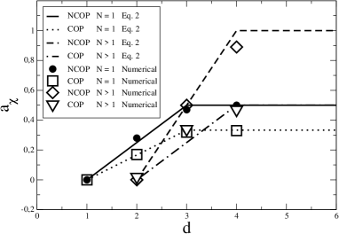
Figure 4: Survey of results in table 2.

The time dependence of $\chi_{ag}(t,t_{w})$ is depicted in Figs. 1, 2 and 3. We have extracted $a_{\chi}$ from the asymptotic power law decay and we have collected all results, old and new, in Table II. At $d_{L}$ we have used the parametric plot $\chi_{ag}(C)$ (insets of Figs. 1, 2 and 3), showing more effectively the absence of asymptotic decay, due to $a_{\chi}=0$. In Table II, we have also reported the values of $a_{\chi}$ predicted by Eq. (2). The comparison with the computed values is quite good. For convenience, we have collected in Table III the values of all the parameters entering Eq. (2). Finally, Fig. 4 provides the pictorial representation of Table II, and it is the main result in the paper.

Let us now comment the results. From Fig. 4 it is evident that the pattern of behavior predicted by Eq. (2) is obeyed with good accuracy in the scalar cases, with $d_{L}=1$ and $d_{U}=3$. In the vector cases, given the great numerical effort needed, values of $N$ were chosen according to the criterion of the best numerical efficiency, together with the requirement to simulate both systems with ($N<d$) and without ($N>d$) stable topological defects. The overall behavior of the data in Fig. 4 shows that Eq. (2) well represents the dimensionality dependence of $a_{\chi}$ also in the vector case with $d_{L}=2$ and $d_{U}=4$. Finally, the insets in Figs 1, 2 and 3 (together with the analogous figures for the $d=1$ Ising model in Ref.s Lippiello2000 ; Castellano and in the large $N$ model Corberi2002 ) show quite clearly that $a_{\chi}=0$ and a non flat FDR are common features in phase ordering kinetics at $d_{L}$.

At this stage Eq. (2) is a phenomenological formula. Apart from the exact solution of the large $N$ model Corberi2002 , there is no derivation of Eq. (2). Here we propose an argument for the dependence of $a_{\chi}$ on $d$ in the scalar case. It is based on two simple physical ingredients: a) the aging response is given by the density of defects $\rho(t)$ times the response of a single defect Corberi2001 $\chi_{ag}(t,t_{w})=\rho(t)\chi_{ag}^{s}(t,t_{w})$ and b) each defect responds to the perturbation by optimizing its position with respect to the external field in a quasi-equilibrium way. In $d=1$ this occurs via a displacement of the defect. In higher dimensions, since defects are spatially extended, the response is produced by a deformation of the defect shape.

We develop the argument for a 2-d system, the extension to arbitrary $d$ being straightforward. A defect is a sharp interface separating two domains of opposite magnetization. In order to analyse $\chi_{ag}^{s}(t,t_{w})$ we consider configurations with a single defect as depicted in Fig. 5. The corresponding integrated response function reads Corberi2001 $\chi_{ag}^{s}(t,t_{w})=1/(h^{2}{\cal L}^{d-1})\int dxdy\,\overline{\langle S(x,y)\rangle h(x,y)}$, where $S(x,y)$ is the order parameter field which saturates to $\pm 1$ in the bulk of domains. $h(x,y)$ is the external random field with expectations $\overline{h(x,y)}=0$, $\overline{h(x,y)h(x^{\prime},y^{\prime})}=h^{2}\delta(x-x^{\prime})\delta(y-y^{\prime})$ and ${\cal L}$ is the linear system size. The overbar and angular brackets denote averages over the random field and thermal histories, respectively. With an interface of shape $z_{w}(y)$ at time $t_{w}$ (Fig. 5), we can write $\chi_{ag}^{s}(t,t_{w})=-1/(h^{2}{\cal L}^{d-1})\overline{\int_{\{z\}}E_{h}\,P_{h}(\{z(y)\},t)}$, where $P_{h}(\{z(y)\},t)$ is the probability that an interface profile $\{z(y)\}$ occurs at time $t$ and $E_{h}=-\int_{0}^{\cal L}dy\int_{z_{w}(y)}^{z(y)}dxh(x,y)\mbox{sign}[z(y)-z_{w}(y)]$ is the magnetic energy. We now introduce assumption b) making the ansatz for the correction to the unperturbed probability $P_{0}(\{z(y)\},t)$ in the form of a Boltzmann factor $P_{h}(\{z(y)\},t)=P_{0}(\{z(y)\},t)\exp(-\beta E_{h})\simeq P_{0}(\{z(y)\},t)[1-\beta E_{h}]$. Then $\chi_{ag}^{s}(t,t_{w})=-1/(h^{2}{\cal L}^{d-1})\overline{\int_{\{z\}}E_{h}(1-\beta E_{h})P_{0}(\{z(y)\},t)}$. Taking into account that the term linear in $E_{h}$ vanishes by symmetry and neglecting $z_{w}(y)$ with respect to $z(y)$ for $t\gg t_{w}$, we eventually find $\beta^{-1}\chi_{ag}^{s}(t,t_{w})={\cal L}^{1-d}\int_{\{z\}}\int_{0}^{\cal L}dy|z(y)|P_{0}(\{z(y)\},t)$. This defines a length which scales as the roughness of the interface Henkel2003 given by $W(t)=[{\cal L}^{1-d}\int_{\{z\}}\int dyz(y)^{2}P_{0}(\{z(y)\},t)]^{1/2}$. The behavior of $W(t)$ in the coarsening process can be inferred from an argument due to Villain Abraham89 . In the case $d\leq 3$, when interfaces are rough Rough , for NCOP one has $W(t)\sim t^{(3-d)/4}$, while for COP $W(t)\sim t^{(3-d)/6}$, with logarithmic corrections in both cases for $d=3$. For $d>3$ interfaces are flat and $W(t)\simeq const.$ Finally, multiplying $\chi_{ag}^{s}$ by $\rho(t)\sim L(t)^{-1}$ Eq. (2) is recovered note2 and $d_{U}$ is identified with the roughening dimensionality $d_{R}=3$. The relevance of roughening in the large time behavior of $\chi(t,t_{w})$ has been independently pointed out by Henkel, Paessens and Pleimling in Ref. Henkel2003 . The crucial difference with these authors is that they believe roughening to be unrelated to aging behavior, while we claim the opposite.

In summary, we have investigated the scaling properties of the response function over a large variety of systems designed to bring forward the generic features when relaxation is driven by coarsening. The primary result is that the exponent $a_{\chi}$ depends on dimensionality and that it vanishes smoothly as $d\rightarrow d_{L}$. This implies that a non trivial FDR is not exceptional, rather is the rule for coarsening systems at $d_{L}$. Another important consequence is that the failure of the connection between statics and dynamics at $d_{L}$ Corberi2001 is also a generic feature of coarsening. The connection between the FDR and the overlap probability function is derived Franz98 under the assumptions of stochastic stability and that $\chi(t,t_{w})$ goes to the equilibrium value as $t\rightarrow\infty$. The latter assumption does not hold at $d_{L}$ due to the existence of a non flat FDR (insets of Figs 1,2,3), which makes the limiting value of $\chi(t,t_{w})$ to rise above the equilibrium value. Obviously, the important and, as of yet, unanswered question is why all this happens at $d_{L}$. The scaling behavior of the response function reported in this Letter adds to the many already existing challenges posed by a theory of phase ordering kinetics.

This work has been partially supported from MURST through PRIN-2002.

	NCOP		COP
$d$	$N=1$	$N>1$	$N=1$	$N>1$
1	$\bullet$		$\bullet$
2	$\bullet$	$N=10$	$N=1$	$N=4$
3	$\bullet$	$N=2$, $N=5$	$N=1$	$N=5$
4	$\bullet$	$N=6$	$N=1$

Table 1: The manifold of systems considered. Entries with dots correspond to systems studied in Refs. Lippiello2000 ; Corberi2001 ; Castellano ; Corberi2003 .

	$N=1$				$N>1$
	NCOP		COP		NCOP		COP
$d$	Eq. (2)	Best fit	Eq. (2).	Best fit	Eq. (2)	Best fit	Eq. (2)	Best fit
1	0	0 $\bullet$	0	0 $\bullet$
2	1/4	0.28 $\bullet$	1/6	0.17	0	-0.07	0	-0.13
3	1/2 $(\log)$	0.47 $\bullet$	1/3 $(\log)$	0.32	1/2	0.50	1/4	0.34
4	1/2	0.50 $\bullet$	1/3	0.33	1 $(\log)$	0.89	1/2 $(\log)$	0.47

Table 2: Exponent $a_{\chi}$ from Eq. (2) and from best fit of numerical data. Values marked by a dot come from Refs. Lippiello2000 ; Corberi2001 ; Castellano ; Corberi2003 .

	$N=1$		$N>1$
	NCOP	COP	NCOP	COP
z	2	3	2	4
$\delta$	1/2	1/3	1	1/2
$d_{L}$	1		2
$d_{U}$	3		4

Table 3: Parameters entering Eq. (2).

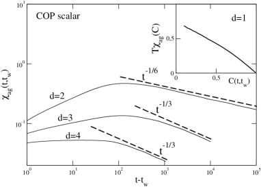
Figure 1: $\chi_{ag}(t,t_{w})$ against $t-t_{w}$ for $N=1$ with COP. Lattice sizes, realizations and $t_{w}$: $512^{2}$, $41$ and $30$ for $d=2$; $128^{3}$, $39$ and $40$ for $d=3$; $60^{4}$, $6$ and $31$ for $d=4$. The dashed lines are the slopes from Eq. (2). In the inset parametric plot for $d=1$ from Ref. Castellano

.

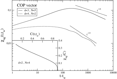
Figure 2: $\chi_{ag}(t,t_{w})$ against $t-t_{w}$ with COP. Lattice sizes, realizations and $t_{w}$: $96^{3}$, $89$ and $35$ for $d=3$ and $N=5$; $50^{4}$, $82$ and $35$ for $d=4$ and $N=2$. The dashed lines are the slopes from Eq. (2). In the inset parametric plot for $d=2,N=4$. Lattice size, realizations and $t_{w}$: $512^{2}$, $232$, $500$).

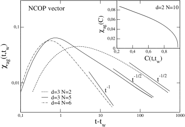
Figure 3: $\chi_{ag}(t,t_{w})$ against $t-t_{w}$ with NCOP. Lattice sizes, realizations and $t_{w}$: $180^{3}$, $1445$ and $2$ for $d=3$ and $N=2$; $140^{3}$, $1486$ and $0.3$ for $d=3$ and $N=5$; $40^{4}$, $486$ and $0.3$ for $d=4$ and $N=6$. In the inset parametric plot for $d=2$ and $N=10$. Lattice size, realizations and $t_{w}$: $1024^{2}$, $22$ and $20$).

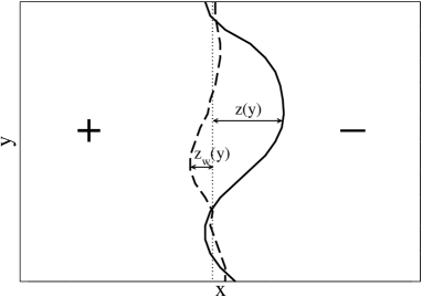
Figure 5: Configurations with a single interface at time $t_{w}$ (dashed line) and at time $t$ (continuous line).

References

- (1) L.F. Cugliandolo and J. Kurchan, Phys. Rev. Lett. 71, 173 (1993); J. Phys. A 31, 5749 (1994).
- (2) For a recent reviews see L. F. Cugliandolo, Dynamics of glassy systems, cond-mat/0210312; A. Crisanti and F. Ritort, J. Phys. A 36, R181 (2003).
- (3) G. Parisi, F. Ricci-Tersenghi and J.J. Ruiz-Lorenzo, Eur. Phys. J. B 11, 317 (1999); J.J. Ruiz-Lorenzo, cond-mat/0306675.
- (4) A.J. Bray, Adv. Phys. 43, 357 (1994).
- (5) E. Lippiello and M. Zannetti, Phys. Rev. E 61, 3369 (2000).
- (6) F. Corberi, E. Lippiello and M. Zannetti, Phys. Rev. E 63, 061506 (2001); F. Corberi, E. Lippiello and M. Zannetti, Eur. Phys. J. B 24, 359 (2001).
- (7) F. Corberi, C. Castellano, E. Lippiello and M. Zannetti, Phys. Rev. E 65, 066114 (2002).
- (8) F. Corberi, E. Lippiello and M. Zannetti, Phys. Rev. Lett. 90, 099601 (2003); F. Corberi, E. Lippiello and M. Zannetti, cond-mat/0307542.
- (9) F. Corberi, E. Lippiello and M. Zannetti, Phys. Rev. E 65, 046136 (2002).
- (10) A. Barrat, Phys. Rev. E 57, 3629 (1998);
- (11) S. Franz, M. Mezard, G. Parisi and L. Peliti, Phys. Rev. Lett. 81, 1758 (1998); J. Stat. Phys. 97, 459 (1999).
- (12) C. Godrèche and J. M. Luck, J. Phys. A 33, 1151 (2000).
- (13) A. J. Bray and K. Humayun, J. Phys. A 23, 5897 (1990).
- (14) The algorithm by Bray and Humayun enters the scaling regime earlier than the GL equations, so that a sufficiently long scaling window exists before finite size effects appear.
- (15) In it is proportional to the displacement of the interface, see Corberi2001 .
- (16) A.-L. Barabási and H. E. Stanley, Fractal Concepts in Surface Growth, (Cambridge University Press, Cambridge, 1995).
- (17) The argument is quoted in D. B. Abraham and P. J. Upton, Phys. Rev. B 39, 736 (1989).
- (18) This argument holds also for Ising spins. Only for differences arise when the Ising model undergoes a roughening transition at the temperature between a low phase with flat (faceted) domain walls and a rough high phase [see T. Emig and T. Nattermann, Eur. Phys. J. B 8, 525 (1999).] Hence we expect logarithmic corrections in Eq. (2) only for , and a pure algebraic decay with for . A numerical test of this prediction would be of great interest, but very demanding from the computational point of view.
- (19) M. Henkel, M. Paessens and M. Pleimling, cond-mat/0310761.