Multidimensional solitons in a low-dimensional periodic potential

Abstract

Using the variational approximation(VA) and direct simulations, we find stable 2D and 3D solitons in the self-attractive Gross-Pitaevskii equation (GPE) with a potential which is uniform in one direction ($z$) and periodic in the others (but the quasi-1D potentials cannot stabilize 3D solitons). The family of solitons includes single- and multi-peaked ones. The results apply to Bose-Einstein condensates (BECs) in optical lattices (OLs), and to spatial or spatiotemporal solitons in layered optical media. This is the first prediction of mobile 2D and 3D solitons in BECs, as they keep mobility along $z$. Head-on collisions of in-phase solitons lead to their fusion into a collapsing pulse. Solitons colliding in adjacent OL-induced channels may form a bound state (BS), which then relaxes to a stable asymmetric form. An initially unstable soliton splits into a three-soliton BS. Localized states in the self-repulsive GPE with the low-dimensional OL are found too.

PACS numbers: 03.75.Fi, 05.30.Jp, 05.45.-a

Introduction. Solitons in multidimensional nonlinear Schrödinger equations (NLSEs) with a periodic potential have recently attracted considerable interest. In particular, self-trapping of spatial beams in nonlinear photonic crystals is described by a 2D equation. In this case, despite the possibility of collapse [1], simulations reveal robust 2D solitons in the self-focusing model [2]. A similar medium can be created by a grid of laser beams illuminating a photorefractive sample [3].

Similar 2D and 3D models with a periodic potential describe a Bose-Einstein condensate (BEC) trapped in an optical lattice (OL) [4]; this application is relevant, as experimental techniques for loading BECs into multidimensional OLs were recently developed [5]. Stable solitons can be supported by an OL even in self-repulsive BECs [6, 7]. In the case of self-attraction, 2D and 3D solitons (including 2D vortices) are stable in the self-focusing model with the OL potential [8], despite the possibility of the collapse.

An issue of direct physical relevance, and a subject of the present work, are multidimensional solitons in media equipped with periodic potentials of a lower dimension, viz., quasi-1D (Q1D) and Q2D lattices in the 2D and 3D cases, respectively. In optics, the 2D equation in the spatial domain governs the beam propagation in a layered bulk medium along the layers, which is an extension of a 1D multichannel system introduced in Ref. [9], where the potential was induced by transverse modulation of the refractive index (RI). In the temporal domain, the 2D and 3D equations govern, respectively, the longitudinal propagation of spatiotemporal optical solitons in a layered planar waveguide, or in a bulk medium with the RI periodically modulated in both transverse directions. The 2D and 3D cases directly apply to BECs loaded in a Q1D or Q2D lattice. The physical significance of this setting is two-fold: first, in the experiment it is much easier to create a lower-dimensional lattice than a full-dimensional one, both in BECs and in optics, hence the use of such lattices is the most straightforward way to create multidimensional solitons in these media. Second, the solitons created this way can freely move in the unconfined direction, which also suggests a possibility to study their collisions, and to look for their bound states (BSs). As yet, no other way to create multidimensional mobile solitons in BECs and their BSs has been proposed. In optics, solitons of this type suggest new applications. Indeed, in an optical medium with the full-dimensional periodic potential, transfer of a trapped beam from one position to another is difficult, as the necessary external push strongly disturbs the beam [9]. In the lower-dimensional potential, the beam can slide along the free direction, making the transfer easy. In BECs confined by a low-dimensional OL, matter-wave solitons can be driven in the free direction by a weak laser beam.

The model and VA. The normalized form of the self-focusing 2D NLSE with a Q1D periodic potential of the strength $\varepsilon$ is

$$iu_{t}+u_{xx}+u_{yy}+[\varepsilon\cos(2x)+\chi|u|^{2}]u=0,$$ (1)

where $\chi=\pm 1$ in the case of the self-attraction/repulsion. In BECs, $t$ is time, while in optics it is the propagation distance. For BECs or spatial optical solitons, $x$ and $y$ are transverse coordinates; for spatiotemporal optical solitons in a 2D waveguide with anomalous chromatic dispersion, $y$ is a temporal variable. The 3D version of Eq. (1) is

$$iu_{t}+u_{xx}+u_{yy}+u_{zz}+\left\{\varepsilon\left[\cos(2x)+\cos(2y)\right]+\chi|u|^{2}\right\}u=0.$$ (2)

Equations (1) and (2) conserve the Hamiltonian, the norm $N=\int\left|u({\bf r})\right|^{2}d{\bf r}\,$ (the number of atoms in the BEC, or total power/energy of the spatial/spatiotemporal optical soliton), and the momentum along the free direction. The equations are normalized so that the period of the potential is $\pi$, the free parameters being $\varepsilon$ and $N$.

Stationary solutions to Eq. (1) are looked for as $u(x,y,t)=U(x,y)\exp(-i\mu t)$, with a chemical potential $\mu$ (propagation constant, in optics), which yields

$$\mu U+U_{xx}+U_{yy}+\left[\varepsilon\cos(2x)+\chi U^{2}\right]U=0,$$ (3)

and similar in the 3D case. To apply the VA (variational approximation) to Eq. (3), we adopt the ansatz $U=A\exp\left[-\left(ax^{2}+by^{2}\right)/2\right]$, or $U=A\exp\left[-\left(a(x^{2}+y^{2})+bz^{2}\right)/2\right]$ in the 3D case, with the norms $N_{2{\rm D}}=\pi A^{2}/\sqrt{ab}$, and $N_{3{\rm D}}=\pi^{3/2}A^{2}/(a\sqrt{b})$. Following the procedure of the application of VA to multidimensional solitons [10], we derive variational equations from the Lagrangian of Eq. (3). In the 2D case, they are ($\aleph\equiv e^{-1/a}$)

$$N\chi=\left(4\pi/a\right)\sqrt{a^{2}-2\varepsilon\aleph},~{}\mu=-a-\varepsilon\aleph(1-3/a),$$ (4)

and in the 3D case [in both cases, $b=\left(a^{2}-2\varepsilon\aleph\right)/a$],

$$N\chi=2\left(2\pi/a\right)^{3/2}\sqrt{a^{2}-2\varepsilon\aleph},~{}\mu=-a/2-\varepsilon\aleph\left(2-3/a\right).$$ (5)

Evidently, solutions are possible only if $\chi>0$ (self-attraction). The 2D solutions exist in the interval

$$N_{\min}\equiv 4\pi\sqrt{1-\varepsilon/\varepsilon_{{\rm cr}}}<N<N_{\max}\equiv 4\pi$$ (6)

[see Fig. 1(a)], if $\varepsilon<\varepsilon_{{\rm cr}}\equiv e^{2}/8\approx\allowbreak 0.924$ ($N_{\min}=0$ if $\varepsilon>\varepsilon_{{\rm cr}}$), while 3D solutions can be found for any $N$. The fixed lattice period rules out establishing general scaling relations for these soliton families; in the case of very large $\varepsilon$, the potential valleys become isolated, then one is actually dealing with cigar-shaped [11] Q1D solitons, that obey the usual 1D NLSE scaling.

The solution families which definitely meet the condition $d\mu/dN<0$ are expected to be stable pursuant to the Vakhitov-Kolokolov (VK) criterion [12], while ones with $d\mu/dN$ positive or nearly zero should be unstable. It follows from Eqs. (4) and (5) and is evident in Figs. 1(b,c) that the 2D solitons are stable in the existence interval (6). At small $\varepsilon$, the 3D solutions are unstable for any $N$. Equation (5) predicts that a stability interval of a width $\Delta N\sim\sqrt{\varepsilon-\varepsilon_{0}}$ appears around $N_{0}\approx 10.1\pi^{3/2}$ if $\varepsilon$ exceeds $\varepsilon_{0}\approx 0.242$.

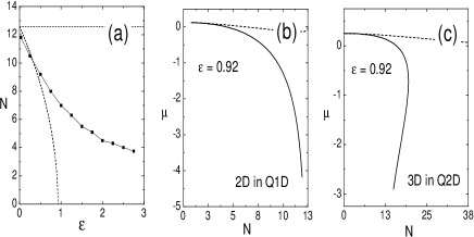
FIG. 1.: The numerically found (joined squares) and VA-predicted (dashed lines) existence limits for stable 2D solitons (a). VA-predicted dependences $\mu(N)$ for the 2D (b) and 3D (c) solitons, which determine their VK stability.

Numerical results. Solitons are generated by the imaginary-time evolution method [13], starting with the VA-predicted waveforms. Stability is verified by direct simulations of perturbed solitons in real time. Typical examples of the thus found stable 2D and 3D solitons are displayed in Fig. 2 and 3, the 3D ones being nearly isotropic in the $\left(x,y\right)$ plane and elongated in the free direction $z$. As is seen in Fig. 1(a), the existence limits for the stable 2D solitons are close to the VA prediction, unless $N$ is small; in that case, the discrepancy is due to the fact that the soliton develops a multi-peaked structure [Fig. 2(b)], which is not accounted for by the simple ansatz adopted above. The ansatz can be generalized for this case, setting $U=\left(A+B\,\cos x\right)\exp\left[-\left(ax^{2}+by^{2}\right)/2\right]$, but the final result is then quite messy. A numerically found stability region for the 3D solitons is also quite close to the VA prediction, and multi-peaked 3D solitons relate to their single-peaked counterparts (Fig. 3) the same way as Fig. 2(b) to Fig. 2(a).

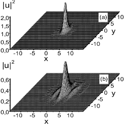
FIG. 2.: Examples of single- and multi-peaked stable 2D solitons in the Q1D potential ($\varepsilon=2$). The norm of the soliton is $N=2\pi$ (a) and $N=1.5\pi$ (b).

The VA predicts that, in the 3D case with the Q1D (rather than Q2D) lattice, all the solitons are VK-unstable. Accordingly, simulations never produced stable solitons in this case. This feature can be explained by the fact that, in the free 2D subspace, the soliton is essentially tantamount to the unstable Townes soliton [1]. In the 2D NLSE with the 2D lattice, stable solitons with intrinsic vorticity were also found in Ref. [8]. Vortices were found in the present 2D model too, but they are always unstable.

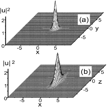
FIG. 3.: A stable single-peaked 3D soliton in the Q2D potential ($N=2\pi$, $\varepsilon=5.0$) is shown through its $z=0$ (a) and $y=0$ (b) cross sections.

We have also investigated the case of self-repulsion, $\chi=-1$, when the low-dimensional lattice potential cannot support a completely localized pulse. However, adding a usual parabolic trap readily gives rise to stable states, which are solitons across the lattice and Thomas-Fermi states along the free direction. It is noteworthy that, with $\chi<0$, these states assume a multi-peaked or single-peaked shape under the action of a weaker or stronger OL potential, respectively, which is opposite to what was reported above for $\chi>0$, cf. Fig. 2. An explanation is that, in the case of the self-repulsion and $\varepsilon=0$, no solitons exist (even unstable ones, like the above-mentioned Townes soliton).

The influence of the parabolic trap was checked too in the case of $\chi=+1$. If the 2D or 3D soliton is displaced from the central position, it performs harmonic oscillations along the free direction, completely preserving its integrity. Actually, the mobility in the free direction is the most essential difference of the present multidimensional solitons from those predicted in other BEC models [6, 7, 8]. This suggests new possibilities, such as collisions between moving solitons.

Simulations demonstrate that 2D and 3D in-phase solitons which collide head-on with velocities $\pm v$, which are below a critical value $v_{{\rm c}}$, merge into a single pulse, whose norm exceeds the critical value $N_{\max}$ [see Eq. (6)], hence it quickly collapses. If $v>v_{{\rm c}}$, the solitons pass through each other (for instance, $v_{{\rm c}}=8.5$ for $\varepsilon=2.0$, when the norm of each 2D soliton is $N=2.5\pi$), which is explained by the fact that the collision time, $\sim 1/v$, is then smaller than the collapse time, $\sim 1/N$. Colliding $\pi$-out-of-phase solitons always bounce back, and two such solitons, placed inside the trap, perform stable oscillations with periodic elastic collisions.

In the low-dimensional potential, collisions are also possible between solitons moving in adjacent “tracks” (channels). In that case, they pass each other quasi-elastically if the collision velocity is large. If it is not too large, each soliton captures a small “satellite” in the other channel. If the velocity falls below a critical value for given $\varepsilon$, the outcome of the collision is altogether different: two solitons form a quiescent symmetric bound state (BS) [Fig. 4(a)]. Later, the symmetric BS develops an intrinsic instability, spontaneously rearranging itself into a completely stable asymmetric BS [Fig. 4(b)]. This behavior resembles the symmetry-breaking instability of optical solitons in dual-core fibers [14] and the macroscopic quantum-self-trapping effect in BECs confined to a double-well potential [15]. In fact, this is the first example of a stable BS of two solitons in BECs. Formation of more complex stable 2D and 3D BSs also occurs in a different way: VK-unstable waveforms predicted by the VA undergo violent evolution, shedding $\simeq 50\%$ of their norm and eventually forming a BS of three solitons, with a narrow tall one in the middle, and small-amplitude broad satellites in the adjacent channels [see Fig. 5].

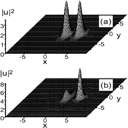
FIG. 4.: A symmetric bound state (BS) of 2D in-phase solitons formed in adjacent tracks as a result of collision between them (a), and its subsequent spontaneous rearrangement into a stable asymmetric BS (b). The initial norm and velocities of the solitons are $N=2\pi$ and $v=\pm 0.1$, and $\varepsilon=3$. In the 3D case, the scenario is quite similar.

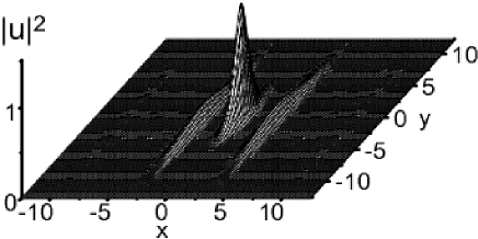
FIG. 5.: Bound state of three solitons developed from the VK - unstable 2D soliton with parameters $A=0.63,\ a=b=0.1$, and $\varepsilon=10$. Half of the initial norm is lost during the formation.

Conclusion. We have demonstrated that the periodic potential whose dimension is smaller by $1$ than the full spatial dimension readily supports stable single- and multi-peaked solitons in 2D and 3D self-focusing media (although the quasi-1D potential cannot stabilize 3D solitons), which suggest new settings for experimental search of solitons. 2D solitons exist in a finite interval of the values of the norm, and 3D ones are stable if the lattice strength exceeds the minimum value. In the case of self-repulsion with a parabolic trap, stable localized states are found too. The dependence of their structure on the lattice strength is opposite to that in the case of the self-attraction: with the increase of the strength, a single-peaked state is changed by a multi-peaked one.

These solitons are the first example of  mobile multi-dimensional pulses in BECs. Head-on collisions between the in-phase solitons may lead to their fusion and collapse, while out-of-phase solitons collide elastically indefinitely many times. Collision between solitons in adjacent tracks may create a bound state (BS), which then relaxes to an asymmetric stable shape. Three-soliton BSs are created as a result of the evolution of initially unstable solitons.

Acknowledgements. We appreciate discussions with Y.S. Kivshar. B.B.B. thanks the Physics Department at the University of Salerno (Italy) for a research grant. B.A.M. appreciates hospitality of the same Department, and partial financial support through the Excellence-Research-Center grant No. 8006/03 from the Israel Science Foundation. M.S. acknowledges partial financial support from the MIUR, through the inter-university project PRIN-2000, and from the European LOCNET grant HPRN-CT-1999-00163.

REFERENCES

- [1] L. Bergé, Phys. Rep. 303, 260 (1998).
- [2] P. Xie, Z.-Q. Zhang, and X. Zhang, Phys. Rev. E 67, 026607 (2003); A. Ferrando et al., Opt. Exp. 11, 452 (2003).
- [3] J. Fleischer et al., Phys. Rev. Lett. 90, 023902 (2003); J. Fleischer et al. Nature, 422, 147 (2003).
- [4] C. Jurczak et al., Phys. Rev. Lett. 77, 1727 (1996); H. Stecher et al., Phys. Rev. A 55, 545 (1997); D. Jaksch et al., Phys. Rev. Lett. 81, 3108 (1998); D. I. Choi and Q. Niu, Phys. Rev. Lett. 82, 2022 (1999); K. P. Marzlin and W. P. Zhang, Phys. Rev. A 59, 2982 (1999); J. H. Denschlag et al., J. Phys. B 35, 3095 (2002); Y. B. Band and M. Trippenbach, Phys. Rev. 65, 053602 (2002); I. Carusotto, D. Embriaco, and G. C. La Rocca, Phys. Rev. A 65, 053611 (2002); S. Burger et al., Europhys. Lett. 57, 1 (2002).
- [5] M. Greiner et al., Nature 415, 39 (2002); 419, 51 (2002); I. Bloch et al., Phil. Trans. R. Soc. L. A 361 1409 (2003).
- [6] B. B. Baizakov, V. V. Konotop, and M. Salerno, J. Phys. B 35, 5105 (2002).
- [7] E. A. Ostrovskaya and Y. S. Kivshar, Phys. Rev. Lett. 90, 160407 (2003).
- [8] B. B. Baizakov, B. A. Malomed, and M. Salerno, Europhys. Lett. 63, 642 (2003); some similar results for the 2D case have also been obtained by J. Yang and Z. Musslimani, Opt. Lett. 23, 2094 (2003).
- [9] B. A. Malomed, Z. H. Wang, P. L. Chu, and G. D. Peng, J. Opt. Soc. Am. B 16, 1197 (1999).
- [10] B.A. Malomed et al., Phys. Rev. E 56, 4725 (1997).
- [11] L. Khaykovich et al., Science 296, 1290 (2002); K. E. Strecker et al., Nature 417, 150 (2002).
- [12] M. G. Vakhitov and A. A. Kolokolov, Radiophys. Quantum Electron. 16, 783 (1973).
- [13] M. L. Chiofalo, S. Succi, and P. Tosi, Phys. Rev. E 62, 7438 (2000).
- [14] C. Pare and M. Florjańczyk, Phys. Rev. A 41, 6287 (1990).
- [15] A. Smerzi, S. Fantoni, S. Giovanazzi, and S.R. Shenoy, Phys. Rev. Lett. 79, 4950 (1997); S. Raghavan, A. Smerzi, S. Fantoni, and S.R. Shenoy, Phys. Rev. A59, 620-633 (1999).