Stripe phase: analytical results for weakly coupled repulsive Hubbard model.

Abstract

Motivated by the stripe developments in cuprates, we review some analytical results of our studies of the charge- and spin density modulations (CDW and SDW) in a weakly coupled one dimensional repulsive electron system on a lattice. It is shown that close to half filling, in the high temperature regime above the mean field transition temperature, short range repulsions favor charge density fluctuations with wave vectors bearing special relations with those of the spin density fluctuations. In the low temperature regime, not only the wave vectors, but also the mutual phases of the CDW and SDW become coupled due to a quantum interference phenomenon, leading to the stripe phase instability in a quasi one-dimensional repulsive electron system. It is shown that away from half filling periodic lattice potential causes cooperative condensation of the spin and charge superlattices. ”Switching off” this potential causes vanishing of the stripe order. The leading spin-charge coupling term in the effective Landau functional is derived microscopically. Results of the 1D renormalization group (parquet) analysis away from half filling are also presented, which indicate transient-scale correlations resembling the mean-field pattern. Farther, the self-consistent solution for the spin-charge solitonic superstructure in a quasi-one-dimensional electron system is obtained in the framework of the Hubbard model as a function of hole doping and temperature. Possible relationship with the stripe phase correlations observed in high $T_{c}$ cuprates is discussed.

Stripe phases recently observed in doped antiferromagnets (cuprates and nickelates) [1, 2, 3] attract attention to the problem of multi-mode instabilities in the interacting electron systems. Numerical mean-field calculations and phenomenological considerations [4, 5, 6, 7] suggest a universality of the spin-charge mode coupling phenomenon in repulsive electronic systems of different dimensionalities. Hence, analytical mean-field solutions of the multi-mode ordering in 1D system could be revealing with respect to the mechanism of the mode coupling. The mean-field solutions would be essentially dimensional-independent and stabilized in three dimensional model by inter-layer interaction. This review is aimed at discussing some of such solutions.

Inelastic neutron scattering experiments in doped cuprates and nickelates reveal pronounced dynamical spin fluctuations centered at the wave vectors $(1/2\pm\varepsilon,1/2)$ and $(1/2,1/2\pm\varepsilon)$ (in units of $2\pi/a$, $a$ is the lattice constant). These are accompanied by dynamical ‘charge’ (crystal lattice) fluctuations at wave vectors $(\pm 2\varepsilon,0)$ and $(0,\pm 2\varepsilon)$. The characteristic wave vectors of spin and charge are harmonically related via the doping dependent parameter $\varepsilon$, indicating that mode-couplings are important. Similarly, the static stripe phases show the same harmonic relations between the spin- and charge ordering wave vectors, thus confirming an idea that spin-charge mode coupling is a necessary condition for these phases to exist. Recent experiments demonstrate [2, 3] that at least in cuprates one has also to deal with the coupling to a pairing mode. It is proposed [7] that the stripe phase might be a quantum liquid crystal state of electrons possessing at the same time a charge-, antiferromagnetic-, and a superconducting condensates.

Since the stripes have to do with a multi-mode instability, the experimental discovery of static stripes and dynamical stripe fluctuations in cuprates and other doped transition metal oxides [1, 2, 3] put forward the following theoretical problem: a theory characterized by coupled modes must be extracted from a (microscopic) model of an interacting electron system.

Stripe-like instabilities do show up in a variety of theoretical approaches, some of them even preceding the experimental discoveries [4, 5]. However, all of these approaches [4, 5, 6, 7] have in common that they deal with the strong coupling regime at zero temperature, while they rest entirely on numerical calculations. To succeed in the same direction analytically, a microscopic model with weakly interacting electron-quasiparticles has been chosen [9, 10]. In such a model, in order to get at a mean-field ordering transition one limits himself to systems exhibiting near to perfect Fermi surface nesting characteristics. This actually implies the choice of only one dimensional (1D) systems.

At first glance, one may argue here that the infrared fixed point structure of 1D interacting electron systems is well understood [11]-[14]. Namely, it is well established that the zero temperature Luttinger liquid exhibits algebraic long range order in both the spin- and the charge sectors [12]. Nevertheless, the evidence is growing [15] that existing picture is not yet complete. Namely, it is very probable that close to half-filling and for relatively weak interactions the ground state is nothing else than a 1D stripe phase, with a long range order which is destroyed by a marginal quantum fluctuations of the order parameter. It is actually well established, that on the classical level the ground state in this regime is a stripe phase, since the mean-field analysis of Schulz [5] for 2D stripes rests on the nesting features which relate these results with (in depth) a 1D effect. Quantum mechanics is involved, as usual, in admixing of the Goldstone modes of the classical state in the ground state, causing in turn the algebraic long range order.

This review consists of the four main parts. The first two parts deal with just the two ”main” charge- and spin harmonics coupling, while the third and the fourth parts allow for all the rest ”obertones” selfconsistently, thus introducing solitonic superstructures of the electronic charge and spin. Before coming to the body of the derivations, let us make a short outline of the four parts in a more detailed fashion.

The novelty of the approach used in [9] and described below lies in that instead of the conventional expansion in terms of a (small) coupling constant between electrons, one expands perturbatively in the coupling strengths between the different spin- and charge modes. For this purpose the classical nature of the dynamics of the collective modes is used, which has a range of validity in a temperature interval around $T_{MF}$ - the mean-field transition temperature into the ordered state. Thus, the interaction strength between the electrons translates into strength of mode couplings. For relatively weak interactions and ”high” temperatures one expects on physical grounds a hierarchy of mode couplings. The dominant coupling is found between the fundamental spin- and charge modes, just as the $\varepsilon$ spin- and $2\varepsilon$ charge modes of the cuprates. Higher order couplings are responsible for the ”solitonic appearance” of the stripe ground state, discussed in the last part of the paper.

Then, considering the coupled spin- and charge fluctuations above $T_{MF}$, it is possible to integrate out spin (SDW) fluctuations in the presence of the relevant charge (CDW) fluctuations [9]. An effective free energy of the system does posses deep local minima at finite CDW amplitudes with the different wave vectors, but the global minimum still corresponds to no CDW at all.

In the second part, results of the paper [10] are presented, which directly demonstrate appearance of the global minimum of the free energy at finite CDW (and SDW) amplitude below $T_{MF}$ when the mutual phase of the coupled charge- and spin modes is locked for a constructive interference to occur. Hence, a quantum interference mechanism of the stripe phase ordering proposed in [10] is described. In order to carry discussion somewhat beyond the mean-field approach, a new modification of the 1D (”parquet”) renormalization group technique is described, which was first applied in [10] to the case of coupled charge and spin fluctuations incommensurate with the crystal lattice away from half filling. As one would expect on the basis of the well known results for 1D systems mentioned above [11]-[14], there is no four-leg vertex divergence found away from commensurability point in the CDW or SDW channels alone. Nevertheless, introduction of the infinitesimal vertices with the new ”Umklapp wave vector” $2\varepsilon$, brought by the incommensurate CDW mode, causes divergence of the four-leg vertices, thus indicating transient-scale correlations resembling the mean-field stripe pattern.

The last two parts of the review contain results published in [16], as well as the new ones. These concern the self-consistent solutions of the Bogoliubov-de Gennes equations for a repulsive 1D Hubbard Hamiltonian written in the Hartree-Fock approximation at zero- and at a finite temperature. Using methods of the finite band potential theory [17], the coupled solitonic charge- and spin superstructures are described analytically in terms of the Jakobi elliptic functions, which, in turn, represent solutions of the non-linear Schrödinger equations. It is shown that far enough from half filling of the bare single electron band the solitonic superstructures smoothly evolve into two coupled CDW and SDW harmonics, considered in the first two parts of the paper. A decrease of the effective mode coupling constant accompanies this transition.

I Two harmonics approximation: charge fluctuations in the classical limit.

This section is based on the results of the works [9]. Our interest is in the description of the precursor fluctuations in the metallic state of a one dimensional system, at temperatures above the mean-field ordering temperature. For a single mode instability in the weak coupling regime this is well described by RPA. Upon the approach of the mean-field transition, the fluctuations slow down and in the vicinity of the transition the characteristic frequency of the collective fluctuations becomes less than temperature. It was demonstrated by several authors (see e.g. [18] and references therein) that under these circumstances the time dependence of the collective modes can be omitted and instead of calculating the full quantum-mechanical trace a classical average suffices.

Let us now consider the Hubbard Hamiltonian with $U>0$, written in the fermionic second-quantized operators $c_{i,\sigma}$:

$$H=t\sum_{<i,j>\sigma}c_{i,\sigma}^{\dagger}c_{j,\sigma}+U\sum_{i}(\frac{1}{4}\hat{n}_{i}^{2}-(\hat{S}_{i}^{z})^{2})\;,$$ (1)

using $\hat{n}_{i\uparrow}\hat{n}_{i\downarrow}=\frac{1}{4}\hat{n}_{i}^{2}-(\hat{S}_{i}^{z})^{2}$ where $\hat{n}\equiv\hat{n}_{\uparrow}+\hat{n}_{\downarrow}$ is the fermion density and $\hat{S}^{z}$ the $z$-component of the fermion spin. The interaction term can be decoupled by the Hubbard-Stratanovich transformation,

$$exp[-\frac{U}{4}(\hat{n}_{i}^{2}-(\hat{S}_{i}^{z})^{2})]={1\over{\pi U}}\int d\rho_{i}dm_{i}exp[-\frac{1}{U}(\rho_{i}^{2}+m_{i}^{2})+i\rho_{i}\hat{n}_{i}+2m_{i}S^{z}_{i}]\;,$$ (2)

introducing two auxiliary fields, describing the collective charge- ($\rho$) and spin ($m$) fluctuations, respectively. It is noted that at temperatures larger than the mean-field transition only spin amplitude fluctuations matter and difficulties [5] related to the apparent violation of the global $SU(2)$ invariance by Eq. (2) are of no importance. Conventionally, one proceeds by neglecting the charge sector completely, except for the $q=0$ static component of the charge mode causing a shift of the thermodynamic potential. However, since the coupling of the charge- and spin modes is important at low temperatures the question arises how to deal with these couplings in the precursor regime.

Starting with a uniform state, it is not easy to keep track of these mode couplings perturbatively. We assume that both the charge- and spin mode condense at the mean-field transition where the dynamics in both sectors slow down and the quasi static approximation can be applied to either the spin- or the charge modes, or both. Since the spin modes dominate the instability, they should be integrated out as accurately as possible (using RPA) which leaves the charge modes to be taken as the static ones. Neglecting subdominant charge-charge mode couplings, the trace in the partition functional $Z$ can be taken over independent charge modes with wave vector $\delta_{c}$ and amplitude $\rho(\delta_{c})$,

$$\rho_{i}=\rho(\delta_{c})\cos(\delta_{c}x_{i})$$ (3)

and the partition sum can be approximated as,

$$Z\simeq\displaystyle\int d\rho(\delta_{c})d\delta_{c}Z(\rho(\delta_{c}),\delta_{c})$$ (4)

where $Z(\rho(\delta_{c}),\delta_{c})$ is the partition function describing the dynamics in the presence of the static charge density waves:

$$Z(\rho(\delta_{c}),\delta_{c}) = \displaystyle\left\{\displaystyle\int{\cal D}\,m_{i}(\tau)\displaystyle\exp{\left[-\int_{0}^{\beta}\sum_{i}\frac{m_{i}^{2}(\tau)}{4U}d\tau\right]}Z_{m}(\rho(\delta_{c}),\delta_{c})\right\}\times$$ (6)

$$\left\{\displaystyle\int{\cal D}\,m_{i}(\tau)\displaystyle\exp{\left[-\int_{0}^{\beta}\sum_{i}\frac{m_{i}^{2}(\tau)}{4U}d\tau\right]}\right\}^{-1}$$

$$Z_{m}(\rho(\delta_{c}),\delta_{c}) = Tr\displaystyle\left\{\exp{[-\beta H_{o}(\rho(\delta_{c}),\delta_{c})]}T_{\tau}\displaystyle\exp{\left(\int_{0}^{\beta}\sum_{i}[m_{i}(\tau)\hat{S}^{z}_{i}(\tau)]d\tau\displaystyle\right)}\right\}$$ (7)

$$H_{o}(\rho(\delta_{c}),\delta_{c}) = \displaystyle-t\sum_{<i,j>,\sigma}{a}_{i,\sigma}^{\dagger}a_{j,\sigma}-\tilde{\mu}\sum_{i}\hat{n}_{i}+U\sum_{i}\rho_{i}(\hat{n_{i}}-n)/2+\frac{U}{4}\sum_{i}\rho_{i}^{2}$$ (8)

where $\rho_{i}$ is given by Eq. (3) and $n$ is the average number of electrons per site ($\leq 1$), while the chemical potential has been shifted,

$$\tilde{\mu}=\mu-\frac{U}{2}n\;.$$ (9)

Summarizing, Eqs. (3-8) are a good approximation when the following conditions are satisfied simultaneously: (i) the characteristic frequencies of the charge fluctuations should be less than $k_{B}T$, (ii) charge-charge mode couplings can be neglected, (iii) The modes Eq. (3) exhaust the partition sum in so far the collective charge sector is involved. Conditions (i) and (iii) are both controlled by the slowing down associated with the mean-field transition. Although close to the transition it is expected that the fundamental charge- and spin harmonics dominate the thermodynamics, this is not necessarily the case on microscopic scales, and condition (ii) limits the validity of our approach to the weak coupling regime. Self-evidently, because the most important (charge-spin) mode coupling is treated explicitely, the above is a considerable improvement over conventional single-mode weak coupling theory, allowing us to penetrate deeper into the intermediate coupling regime.

A Mode coupling by Fermi-surface matching.

In this section we will further elaborate on the formalism. However, the central outcome of our analysis can already be qualitatively understood at this point: pairs of charge- and spin fluctuations with special relationships between their momenta are simultaneously enhanced in the approach to the transition. These include the $\varepsilon$-spin and $2\varepsilon$ charge fluctuations reminescent of the stripe fluctuations in cuprates. In addition, there is actually an infinite progression of these pairs, although the enhancement factors rapidly decrease upon going to higher orders. The mechanism is straightforward : by repeated Umklapp scatterings against the CDW, a non-$2k_{F}$ SDW can ‘borrow’ the momentum mismatch with regard to the $2k_{F}$ nesting vector from the CDW. Obviously, this can only happen if special relations exist between the wave vectors of the SDW and CDW.

Close to the transition, the spin fluctuation can be considered as static, as the static charge density wave Eq. (3). Due to the underlying lattice periodicity a spin-density wave is of the form

$$S(x)=\displaystyle S_{0}\cos(\delta_{s}x)\sin(\frac{\pi x}{a})=S_{o}\frac{1}{2}\left[\sin(xk_{-})+\sin(xk_{+})\right]$$ (10)

with $k_{\pm}=\pi/a\pm\delta_{s}$. The two terms in the brackets in Eq. (10) have a straightforward meaning. The first one arises due to the back-scattering of the fermion with a momentum change of $k_{-}$, while the second term comes from Umklapp scattering with a total momentum change $2\pi/a-k_{-}\equiv k_{+}$. On the other hand, assuming linear fermion dispersions the Fermi-momentum can be written in the proximity of half-filling as,

$$k_{F}=\frac{\pi}{2a}-\frac{\delta}{2}\;;\;\frac{\delta}{2}\equiv x_{d}\frac{\pi}{2a}$$ (11)

where $x_{d}$ is the (hole) doping concentration (at half-filling, $k_{F}=\pi/(2a)$ ).

We have introduced intentionally three different momenta: $\delta$, the deviation of $k_{F}$ from its half-filled value, and the wavectors associated with the modulation of the Néel state ($\delta_{s}$) and with the charge modulation ($\delta_{c}$), respectively. Only in the absence of the CDW, the SDW wave vector $k_{-}$ equals $2k_{F}=\pi/a-\delta\equiv\pi/a-\delta_{s}$. In the presence of the CDW, however, a whole variety of new possibilities arises. According to Eq. (8 ), the fermion momentum is conserved only modulo $m\times\delta_{c}$, $m=\pm 1,\pm 2$,…, because of the presence of the periodic potential produced by the CDW. This adds new umklapp scattering vectors, which are linear combinations of the vectors $2\pi/a$ and $\delta_{c}$. Therefore, $2k_{F}$ may now differ from either $k_{-}$ or $k_{+}$ by an integer number of CDW wave vectors: $k_{-}-2k_{F}=m\delta_{c};\;m=0,\pm 1,...$; $k_{+}-2k_{F}=n\delta_{c};\;n=0,1,...$. Notice that the summation over $n$ is restricted to positive integers to avoid redundancy in the counting of the allowed SDW wave vectors. These relations are equivalent to,

$$\delta-\delta_{s}=m\delta_{c}\;;\;\;m=0,\pm 1,\pm 2,...$$ (12)

$$\delta+\delta_{s}=n\delta_{c}\;;\;\;n=1,2,...$$ (13)

It follows immediately that both relations are only fulfilled simultaneously for the following ”matching pairs” of wave vectors $\delta_{c}$ and $\delta_{s}$,

$$\displaystyle\left\{\begin{array}[]{c}\delta_{c}=\displaystyle\frac{2\delta}{n-m}\\ \\ \;\;\;\delta_{s}=\displaystyle\frac{(m+n)\delta}{n-m}\end{array}\right.$$ (17)

where $|m|<n\;;m=0,\pm 1,\pm 2,...\;;n=1,2,...$. The distinction between the matching pairs in Eq. (17) and other pairs $\delta_{c}$ and $\delta_{s}$, obeying only one of the two relations in Eq. (13) will become apparent in the next subsection. Notice that the symmetry relations expressed in Eqs. (13-17) are not related to the actual values of $t$ and $U$ in the Hamiltonian Eq. (1), as long as the fermion dispersions are linear and the two-mode approximation (one SDW and one CDW) is valid. In combination, this limits the present approach to relatively weak couplings. We will elobarate this further in the next sections.

B Free energy of the SDW-CDW fluctuations

Let us proceed to derive the fluctuation contribution to the free energy, in order to see how the relations Eqs. (13,17) follow from the thermodynamics of the electron system described by Eqs. (3-8). For this purpose, the spin fluctuations in the presence of the CDW, as described by Eqs. (6-8) will be integrated out on the RPA level. We proceed by calculating the free energy functional for fixed charge modulations,

$$\Omega(\rho(\delta_{c}),\delta_{c})=-T\ln Z(\rho(\delta_{c}),\delta_{c})\;,$$ (18)

with $Z(\rho(\delta_{c}),\delta_{c})$ defined in Eq. (6) and the total partition sum Eq. (4) becomes,

$$Z=\int d\delta_{c}\int d\rho(\delta_{z})\exp(-\beta\Omega(\rho(\delta_{c}),\delta_{c}))$$ (19)

In the single-loop approximation, $Z_{m}(\rho(\delta_{c}),\delta_{c})$ in Eq. (7) becomes

$$Z_{m}(\rho(\delta_{c}),\delta_{c}) = \displaystyle\exp\{-\beta(\Omega_{o}+\Omega_{m})\}\;;\;\Omega_{o}\approx\frac{U(1-U\nu(\tilde{\mu}))}{4}\sum_{i}\rho_{i}^{2}+\Omega_{b}$$ (20)

$$\displaystyle\beta\Omega_{m} = -\frac{1}{2}\int_{0}^{\beta}\int_{0}^{\beta}d\,\tau_{1}d\,\tau_{2}\sum_{i_{1},i_{2}}m_{i_{1}}(\tau_{1})m_{i_{2}}(\tau_{2})\langle T_{\tau}\hat{S}^{z}_{i_{1}}(\tau_{1})\hat{S}^{z}_{i_{2}}(\tau_{2})\rangle$$ (21)

$$= \displaystyle-\sum_{\omega_{n},\vec{q}}m(\vec{q},\omega_{n})m(-\vec{q},-\omega_{n})\chi(\vec{q},\omega_{n})\;,$$ (22)

where $\nu(\tilde{\mu})$ is the density of states at the Fermi level, and $\chi(\vec{q},\omega_{n})$ the Fourier component of the magnetic susceptibility of the system calculated with the Hamiltonian Eq. (8), i.e. in the presence of the charge density modulation $\rho_{i}$, Eq. (3). $m(\vec{q},\omega_{n})$ corresponds with the Fourier component of the Hubbard-Stratonovich spin field at momentum $q$ and Matsubara frequency $\omega_{n}$[19]. Finally, $\Omega_{b}$ is a background contribution which is independent of $\rho_{i}$ and $m$. Substituting Eqs. (20,22) into Eqs. (6,7) and carrying out a Gaussian integration over the real and imaginary parts of the Fourier components $m(\vec{q},\omega_{n})$ we arrive at the following expression for the free energy functional Eq.(18),

$$\Omega(\rho(\delta_{c}),\delta_{c})=\displaystyle\frac{U(1-U\nu(\tilde{\mu}))}{4}\sum_{i}\rho(\delta_{c})^{2}+\Omega_{b}+TN\sum_{\omega_{n},\vec{q}}\ln{(1-U\chi(\vec{q},\omega_{n}))}$$ (23)

Dropping as usually [18] all the terms with $\omega_{n}\neq 0$, the semi-static part of the free energy functional (per lattice site) $\tilde{\Omega}$ is found, depending on the CDW with wave vector $\delta_{c}$ and amplitude $\rho(\delta_{c})$,

$$\tilde{\Omega}(\rho(\delta_{c},\delta_{c})=\displaystyle\frac{U\rho(\delta_{c})^{2}}{4}(1-U\nu(\tilde{\mu}))+T\sum_{q=\pm\delta_{s}}\ln(1-U\chi_{\pi/a+q}(\rho(\delta_{c}),\delta_{c}))+\tilde{\Omega}_{b}\;.$$ (24)

$\tilde{\Omega}_{b}$ absorbs the background contributions and will be neglected in the remainder. The first term describes the potential energy cost of creating a CDW in a system with repulsive interactions, and the second term describes the decrease of the free energy due to the spin density fluctuations with wave vectors $\delta_{s}$ relative to the wave vector of the antiferromagnet at half-filling.

The static magnetic susceptibility $\chi$ in the presence of the periodic CDW potential remains to be calculated. For linearized dispersion of electrons near Fermi momentum it takes the form (compare [20]),

$$\chi_{\pi/a+\delta_{s}}(\rho(\delta_{c}),\delta_{c}) = T\sum_{\omega_{n}}\int d\,x^{\prime}\,\left[\exp\{i(\delta_{s}-\delta)(x-x^{\prime})\}g_{++}(i\omega_{n};x,x^{\prime})g_{--}(i\omega_{n};x^{\prime},x)\right.$$ (26)

$$\left.+(x\leftrightarrow x^{\prime})\right]\;,$$

counting $2k_{F}$ from its commensurate $\pi/a$ value according to Eq. (11). The Green’s function $g_{++}$ ($g_{--}$) is the slowly varying part of the full fermion Green’s function, $G$, in the Matsubara representation for the right (left)-movers. For example,

$$G_{++}(i\omega_{n};x,x^{\prime})=\exp[ik_{F}(x-x^{\prime})]g_{++}(i\omega_{n};x,x^{\prime})\;.$$ (27)

For these Green’s functions we find,

$$g_{++}(i\omega_{n};x,x^{\prime}) = \displaystyle\frac{sign\omega_{n}}{i2t}\exp\left[-\frac{\omega_{n}(x-x^{\prime})}{2t}-\frac{iU}{4t}\int_{x^{\prime}}^{x}\rho(u)d\,u\right];\;\mbox{when $\displaystyle\frac{\omega_{n}(x-x^{\prime})}{2t}>0$}$$ (28)

$$g_{++}(i\omega_{n};x,x^{\prime}) = 0;\;\mbox{when $\displaystyle\frac{\omega_{n}(x-x^{\prime})}{2t}<0$ }$$ (29)

using the shorthand $\rho(u)=\rho(\delta_{c})\cos(\delta_{c}u)$ for the charge modulation. The corresponding Green’s function for the left-movers is derived by changing the sign in front of the $t$ appearing in the argument of the exponent in Eq. (29). Substituting Eq. (29) into Eq. (26), and making use of the identity :

$$\sum_{n=0}^{\infty}\exp{\{-\pi T(2n+1)z\}}\equiv\displaystyle\frac{1}{\sinh{\{\pi Tz}\}};\;\;z>0$$ (30)

one obtains:

$$\chi_{\pi/a+\delta_{s}} = \displaystyle\frac{T}{4t^{2}}Re\left(\int_{1}^{\infty}dz\;\frac{\exp{\left[iz(\delta_{s}-\delta)-\displaystyle\frac{i2U\rho(\delta_{c})}{\delta_{c}t}\sin{(\delta_{c}z/2)}\cos{(\delta_{c}(x-z/2))}\right]}}{\sinh{(\pi Tz/t)}}\right.$$ (32)

$$\displaystyle\left.+\int_{1}^{\infty}dz\;\frac{\exp{\left[iz(\delta_{s}+\delta)+\displaystyle\frac{i2U\rho(\delta_{c})}{\delta_{c}t}\sin{(\delta_{c}z/2)}\cos{(\delta_{c}(x-z/2))}\right]}}{\sinh{(\pi Tz/t)}}\right)$$

where lower cut-off in the integration is taken at the lattice constant $a\equiv 1$. Now, using wellknown property of Bessel functions of integer order:

$$\exp{(iz\cos{\phi})}=\sum_{n=-\infty}^{n=+\infty}i^{n}\exp{(in\phi)}J_{n}(z)$$ (33)

and averaging over the phase (position) of the CDW in Eq. (32) we find:

$$\chi_{\pi/a+\delta_{s}}=\displaystyle\frac{T}{4t^{2}}\int_{1}^{\infty}dz\;\frac{[\cos{(z(\delta_{s}+\delta))}+\cos{(z(\delta_{s}-\delta))}]}{\sinh{(\pi Tz/t)}}J_{0}\left(\frac{2U\rho(\delta_{c})}{\delta_{c}t}\sin{(\delta_{c}z/2)}\right)$$ (34)

Using now the well known [21] addition theorem for Bessel functions of integer order ($J_{n}(x)$), we obtain the key result:

$$\chi_{\pi/a+\delta_{s}}=\displaystyle\frac{T}{4t^{2}}\int_{1}^{\infty}\frac{dz}{\sinh{(\pi Tz/t)}}\left[J_{0}^{2}\left(\frac{U\rho(\delta_{c})}{t\delta_{c}}\right)[\cos{(z(\delta_{s}+\delta))}+\cos{(z(\delta_{s}-\delta))}]\right.$$ (35)

$$\left.+\sum_{n=1}^{\infty}J_{n}^{2}\left(\frac{U\rho(\delta_{c})}{t\delta_{c}}\right)[\cos{(z(\delta_{s}+\delta+n\delta_{c}))}+\cos{(z(\delta_{s}-\delta+n\delta_{c}))}+\cos{(z(\delta_{s}+\delta-n\delta_{c}))}\right.$$ (36)

$$\left.+\cos{(z(\delta_{s}-\delta-n\delta_{c}))}]\displaystyle\right]$$ (37)

Coarse graining of Eq. (37) with respect to the thermal length of electron, $l_{T}=\pi T/t$, leads to the simplified expression ():

$$\chi_{\pi/a+\delta_{s}}(\rho(\delta_{c}),\delta_{c}) = \displaystyle\frac{1}{4\pi t}\ln{\frac{2t}{\pi T}}\left[J_{0}^{2}\left(\frac{U\rho(\delta_{c})}{t\delta_{c}}\right)(\delta_{\delta_{s},\delta}+\delta_{\delta_{s},-\delta})+\sum_{n=1}^{\infty}J_{n}^{2}\left(\frac{U\rho(\delta_{c})}{t\delta_{c}}\right)\right.$$ (39)

$$\left.\times(\delta_{\delta_{s}+\delta,n\delta_{c}}+\delta_{\delta_{s}-\delta,n\delta_{c}}+\delta_{\delta_{s}+\delta,-n\delta_{c}}+\delta_{\delta_{s}-\delta,-n\delta_{c}})\right]\;$$

where $\delta_{\alpha,\beta}$ is the Kronecker symbol. For a zero amplitude of the CDW ($\rho(\delta_{c})=0$), Eq. (39) reduces to the standard weak coupling result[18] and the SDW condensation temperature follows directly,

$$T_{SDW}=\displaystyle\frac{2t}{\pi}\exp{\left(-\frac{4\pi t}{U}\right)}$$ (40)

The picture changes drastically when the CDW’s are allowed to have a finite amplitude. To see what happens, let us introduce the distribution function describing the probability of finding a CDW fluctuation at wave vector $\delta_{c}$,

$$W(\delta_{c})=\displaystyle\int\exp\left\{-\frac{\tilde{\Omega}(\rho(\delta_{c}),\delta_{c})}{T}\right\}d\,\rho(\delta_{c})\left[\displaystyle\int\left(\int\exp\left\{-\frac{\tilde{\Omega}(\rho(\delta_{c}),\delta_{c})}{T}\right\}d\,\rho(\delta_{c})\right)d\,\delta_{c}\right]^{-1}\;,$$ (41)

which was calculated numerically. The effect of the thermal length, $l_{T}$, is effectively excluded in the simplified expression in Eq. (39) (coarse graining procedure) and is present in Eq. (37). This will especially be of importance at large wavelengths, $\delta_{c}<\pi/l_{T}$, diminishing the multiple scatterings of the fermions against the CDW. It is noticed that in this way only an upper bound to the disordering length is incorporated. Correlations are expected to be further reduced by charge-charge mode couplings, etcetera, neglected in the present analysis.

In the figures 1-2 the numerical results following from Eq. (41) are shown for some representative choices of parameters. Namely, in Fig.1 : $x_{d}=0.02,\;U/t=2;\;T=1.2T_{SDW};\;T=2T_{SDW}$. The blue dashed ($T=1.2T_{SDW}$) and red dashed ($T=2T_{SDW}$) curves are obtained using Eq. (39), i.e. when damping effects have been neglected. The blue solid ($T=1.2T_{SDW}$) and red solid ($T=2T_{SDW}$) curves in Fig. 1 were calculated using Eq. (37), i.e. with the thermal length effect of the fermion included. This makes peaks sensitive to the temperature, so that higher the temperature the more substantial becomes smearing of the peaks. Comparing dashed and solid curves we notice that finite thermal length causes merging of the peaks for small values of $\delta_{c}$ (corresponding to $Z_{c}<1$) into one broad feature, while these peaks remain well resolved on the dashed curves at both temperatures chosen. For reasons which will become clear in a moment, the wave vectors are normalized to the Fermi surface spanning vector $\delta$,

$$Z_{c} \equiv {{\delta_{c}}\over{\delta}}$$ (42)

$$Z_{s} \equiv {{\delta_{s}}\over{\delta}}\;.$$ (43)

Let us first consider the undamped case in Fig. 1. Our main result becomes immediately obvious: the charge fluctuations exhibit a highly organized behavior as function of their wave vectors. The large momentum regime is dominated by a peak centered at $Z_{c}=2$, corresponding with CDW wave vector $\delta_{c}=2\delta$ which is reminescent of the stripe-charge fluctuation as seen in cuprates. This fluctuation becomes more significant both for smalller dopings and smaller temperatures.
In addition, a variety of smaller peaks is found which occur at finite CDW amplitudes and at wave vectors which are rational fractions of the Fermi-surface spanning factor $\delta$, i.e. $Z_{c}\equiv\delta_{c}/\delta=n/m$, with $n,m$ integers. Since the fluctuations under $Z_{c}=2$ are not completely unanticipated, these finite amplitude ‘fractional momentum’ charge fluctuations should be viewed as a qualitative novelty, unique to the present analysis. Because they show up at smaller momenta, they are also more susceptible for smearing effects as the comparison with the two solid/dashed curves in Fig. 1 and two curves in Fig. 2 show. At the same time, it might well be that the members of this series with the largest $Z_{c}$’s will survive. Fig. 2 is important for understanding of the Scilla and Horribda situation created by the first two terms in Eq. (24). While the first term suppresses peaks at too high doping due to increase of potential (”Coulomb”) energy cost of a CDW, the second term produces less sharper peaks at too small doping due to thermal length smearing effect at small wave vector value, $\delta_{c}\sim x_{d}$, of a CDW. In order to decrease smearing effect at a fixed doping one has to go to lower temperatures, i.e. smaller $T_{SDW}$, by decreasing $U/t$ ratio. Solid (black)curve in Fig. 2 is obtained for the set of parameters: $x_{d}=0.001,\;U/t=1;\;T=1.2T_{SDW}$. Dotted (red) curve in Fig. 2 is the same as the ”low temperature” (i.e. at $T=1.2T_{SDW}$) solid (blue) curve in Fig. 1, and is drawn for comparison. We see that peak at $\delta_{c}=\delta$ ($Z_{c}=1$) has become well resolved, and both peaks on the solid curve are much sharper than on the dotted one. This means that effect of CDW precursors with discrete wave vectors demonstarted in Fig. 1 becomes well pronounced in the weak coupling-low doping concentration limit.

The attentive reader should already have realized that the above reflects the ‘matching pair’ counting of Section A. Recalling Eq. (17), the first few members of this series are: $\{\delta_{s}=\delta\;,\delta_{c}=2\delta\}$; $\{\delta_{s}=\delta\;,\delta_{c}=\delta\}$; $\{\delta_{s}=\delta\;,\delta_{c}=2\delta/3\}$, and $\{\delta_{s}=\delta\;,\delta_{c}=\delta/2\}$, which corrrespond with the sets of integers : $m=0;\;n=1,2,3,4$. The charge wave vectors are clearly recognized in the figures (except $\delta_{c}=2\delta/3$, which is not seen due to not sufficient sensitivity of the Kronecker symbol simulation routine at $Z_{c}=n/3,\;n=1,2$).

It is instructive to consider how these ‘matching pair’ fluctuations arise in the present calculation. The key is that the CDW fluctuations with a ‘matching’ wave vector lead to a selective enhancement of the spin density fluctuations with proper momenta. The latter push the free-energy downwards, causing pronounced local minima in $\tilde{\Omega}(\rho(\delta_{c},\delta_{c})$ (Eq. 24) which are sufficiently deep to carry appreciable statistical weight in Eq. (41).

The dependence of the free-energy on the CDW wave vector $\delta_{c}$ enters entirely through the generalized Lindhard function, Eqs.(37),(39). The latter depends on this wave vector both through the argument of the Bessel functions, and through the limitations imposed on the summation over the higher order Bessel functions by the Kronecker $\delta$’s, matching the SDW and CDW vectors to the Fermi momentum. On the other hand, the dependence on the amplitude $\rho(\delta_{c})$ enters both through the first term in Eq. (24), describing the restoring force tending to keep the charge density uniform in this repulsive system, and again through the argument of the Bessel functions. The first term $\sim J^{2}_{0}$ in Eq. (39) is non-zero for any CDW wave vector and is responsible for the $\delta_{c}$ independent background. The texture in Figs. 1-2 is caused by the higher order Bessel functions and in order to gain some intuition one has to investigate which values of $\delta_{s}$ contribute to the sum in Eq. (24) at any fixed value of $\delta_{c}$, as well as how differs the actual structure of the expression $\chi_{\delta_{s}}$ in Eq. (39) for the values of $\delta_{c}$, which either belong or do not belong to any matching pair $\{\delta_{c},\delta_{s}\}$. For this purpose the manifold of points $\{\delta_{c},\delta_{s}\}$, which give non-zero contribution into $\chi_{\delta_{s}}$ in Eq. (39), is plotted in Fig. 3 in the coordinates $Z_{c}$, $Z_{s}$. At each point belonging to any straight line in Fig.3 : $Z_{s}\pm 1=n\times Z_{c};\;n=0,\,\pm 1,\,\pm 2\,,...$, an argument of one of the Kronecker’s symbols in Eq. (39) becomes zero . Only Bessel functions of the order $n\leq 8$ were retained in the sum in r.h.s. of Eq. (39) in order to obtain plots in Figs. 1-2. The reason for this is that high order Bessel functions, $J_{n}^{2}(U\rho(\delta_{c})/(t\delta_{c}))$, give negligible contributions to the sum when their argument becomes much less than order $n$. The value of the argument, $z\equiv U\rho(\delta_{c})/(t\delta_{c})$, is limited from above by the condition of the high probability of the related CDW fluctuation: $\tilde{\Omega}(\rho(\delta_{c}),\delta_{c})/T\leq 1$. This condition leads, due to the first term in Eq. (24), to the limitation: $z\leq 4\exp{(-w)}/(\pi x_{d}\sqrt{w})$, where $w\equiv 4\pi t/U$, and the estimates: T $\sim$ T_SDW, $\delta_{c}\sim\delta$ were used. For the range of doping concentrations $x_{d}$ and coupling strengths $w$, which were chosen for the calculations, the last inequality gives $n\,<\,5$. The coordinates of the crossing points of any two lines in fig. 3 determine the matching pairs of CDW-SDW fluctuations with wave-vectors $\{\delta_{c}=Z_{c}\delta,\;\delta_{s}=Z_{s}\delta\}$. In order to see the ”matching - non-matching” distinction in the structure of the expression for $\chi_{\delta_{s}}$ in Eq. (24), Fig. 4 is presented. It shows how many terms are simultaneously non-zero in Eq. (39) at each point, which belongs to the manifold in Fig. 3 and has coordinates $\{Z_{c},\,Z_{s}\}$. The latter manifold was substantially rarefied along $Z_{c}$ (but not along $Z_{s}$ !) axis in order to provide better visibility in Fig. 4. Each solid circle in Fig. 4 indicates that the number of non-zero terms at this particular point is two, while open circles and squares indicate that this number is one. Again, only Bessel functions of the order $n\leq 4$ are accounted for. The solid circles in Fig. 4 coincide with the two line crossing points in Fig. 3. We see that ”columns” of solid circles in Fig. 4 erect only upon the $\delta_{c}$ ($Z_{c}$) values which are members of the matching pairs. The open circles in these columns would be also solid if we would not restrict the order of the Bessel functions in Eq. (39) to $n\leq 8$. The structure of the sum in Eq. (39) described above gives rise to the peaks seen in the W$(Z_{c})$ curves in Figs. 1-2. Finally, the absolute walue of W$(Z_{c})$ is obtained by normalizing to unity on the limited interval of variation of $Z_{c}$. This interval is limited from above by the applicability of the quasi classical approximation for the Green’s functions of electron, i.e. $\delta_{c}\ll\pi/a\sim 2k_{F}$, or in the equivalent form: $Z_{c}\ll 1/x_{d}$. On the other hand, it is seen in Figs. 1-2 that the background part of W$(Z_{c})$ stretches over an interval of $Z_{c}$, which is at least order of magnitude wide, and extrapolates to a non-zero value in the ”forbidden region”, $Z_{c}\sim 1/x_{d}$. This makes normalization procedure somewhat uncertain.

C Discussion: $\delta_{c}=2\delta_{s}$, but $\delta_{s}=x_{d}/2$

Here the main results presented in Section I are summarized and discussed. First of all, we notice that in terms of reciprocal units, $2\pi/a$, the wave vectors of the symmetry coupled SDW and CDW fluctuations, ‘matching pairs’, chosen at the end of the previous subsection, could be expressed as: $1/2\pm\varepsilon$ , $\pm 2\varepsilon$ for the first pair; $1/2\pm\varepsilon$ , $\pm\varepsilon$ for the second pair; $1/2\pm 3\varepsilon$ , $\pm 2\varepsilon$ for the third pair, and $1/2\pm\varepsilon/3$ , $\pm 2\varepsilon/3$ for the fourth matching pair of the wave-vectors $\{\delta_{s},\delta_{c}\}$. Here we have according to Eq. (12): $\varepsilon=a\delta/(2\pi)=x_{d}/2$. The whole picture of the CDW fluctuation loses its sense if the period of the wave, $2\pi/\delta_{c}$, becomes greater than the thermal length, $l_{T}\sim at/(\pi T)$ (compare [18, 20]). Allowing for the fact that the most important values are $\delta_{c}\sim\delta_{s}\sim\delta$ we find that our results are limited to the interval of doping concentrations not too close to half-filling:

$$x_{d}\gg\displaystyle\frac{T}{t}\geq\displaystyle\frac{T_{SDW}}{t}\sim\exp{\left(-\frac{4\pi t}{U}\right)}\;.$$ (44)

On the other hand, in order a nonperturbative nature of CDW potential scattering would come into power and prowide discrete features seen in Figs. 1-2, the potential energy cost of a CDW formation with finite amplitude should not be too high. Namely, the argument of the Bessel functions in Eqs. (37), (39) should be allowed to be of order unity, i.e. $U\rho(\delta_{c})\geq t\delta_{c}$. Substituting then the resulting value of $\rho$: $\rho(\delta_{c})\geq t\delta_{c}/U$, into the potential energy term in Eq. (24) and requiring that it would be less than temperature $T\sim T_{SDW}$ one arrives at the upper bound for $x_{d}$:

$$x_{d}\ll\displaystyle\sqrt{\frac{U}{t}}\exp{\left(-\frac{2\pi t}{U}\right)}\;.$$ (45)

Combining Eqs. (44) and (45) we find an interval of ‘allowed’ values of the doping concentration $x_{d}$, where the ‘matching pairs’ effect could be expected:

$$\exp{\left(-\frac{4\pi t}{U}\right)}\ll x_{d}\ll\displaystyle\sqrt{\frac{U}{t}}\exp{\left(-\frac{2\pi t}{U}\right)}\;.$$ (46)

As the $x_{d}$ interval above is defined purely via $U/t$ ratio, i.e. coupling strength parameter, we see that in fact Eq. (46) defines a region in the phase diagram in the coordinates $x_{d}$, $U/t$, inside which the effect predicted in this paper should take place.

According to Figs. 1-2 the most probable CDW fluctuation at the temperatures T close to T_SDW has wave-vector $\delta_{c}=2\delta$. Also, according to Fig. 3, the lowest order SDW fluctuation coupled to this CDW has wave-vector $\delta_{s}=\delta$. For the system of a 2-dimensional array of weakly coupled chains (parallel to the $x$-axis) this (matching) pair of wave-vectors: $1/2\pm\varepsilon$ and $\pm 2\varepsilon$, translates into a 2-D form: the SDW wave vector is now $(1/2\pm\varepsilon,1/2)$ , and the CDW wave vector is $(\pm 2\varepsilon,0)$, which coincides with the stripe-theory prediction in a moderately strong coupling limit, $U/4t\geq 1$, for the square lattice, [22]. This coincidence is nevertheless quite limited, in the sense that here we have found the most probable configuration of the coupled spin-charge fluctuations above T_SDW (see also ), while theory [22] describes the ground state spin-charge configuration. On the other hand, when translated into 2-D form, our present result is in accord with the inelastic neutron scattering data in underdoped cuprates [1] at the temperatures T greater than superconducting transition temperature T_c. Namely, the most intensive magnetic neutron scattering is measured at 2-D wave-vector $(1/2\pm\varepsilon,\;1/2)$, while scattering of neutrons by the crystal lattice potential (which indirectly reflects the presense of a CDW) has occured at $(\pm 2\varepsilon,\;0)$. Nevertheless, as in the moderately strong coupling stripe theory [22], our prediction for the doping dependence of $\varepsilon$: $\varepsilon=x_{d}/2$, differs by a factor of two relative to the experimental result in cuprates : $\varepsilon=x_{d}$.

II Stripe phase ordering as a quantum interference phenomenon.

The main content of this section is based on the work [10]. It is well established, that in the Galilean invariant 1D system one finds on the mean-field level a single mode Peierls wave [21] with wave vector $2k_{F}$ at arbitrary electron density ($k_{F}$ is the Fermi momentum). It is generally assumed that the same holds true on a 1D lattice away from points of lattice commensuration since then an umklapp scattering of electrons by inverse lattice wave-vector $2\pi/a$ is ineffective [12, 14]. As a result, Peierls state with incommensurate periodic spin density structure (SDW) is predicted in repulsive case both on the mean-field as on the single loop renormalization group (“parquet”) level. In fact this assertion is incorrect. Here we demonstrate that in 1D even in a weak coupling limit, $U/t\rightarrow 0$, the spin-charge modes coupling is relevant at small doping $x_{d}$, i.e. close to half-filling of electron band ($1-x_{d}$ electron per lattice site). The mechanism is genuinely novel [10] and is related to interference phenomenon involving multiple scatterings of electrons by inverse lattice wave-vector and by wave-vector of self-consistently generated charge density mode (CDW). Essential role of the umklapp scattering makes this phenomenon strongly doping-dependent as distinguished from welknown phenomenon of related $2k_{F}$-SDW and $4k_{F}$-CDW fluctuations in a Luttinger liquid [22].

Recently the Landau free-energy functional was phenomenologicallly introduced [23], which contains a leading order mode coupling term between the fundamental Fourier components of the spin ($\vec{S_{q}}$) and charge ($\rho_{k}$) order parameters :

$${\cal{F}}=\frac{1}{2}r_{\rho}|\rho_{k}|^{2}+\frac{1}{2}r_{s}|\vec{S}_{q}|^{2}+\lambda_{1}[(\vec{S}_{q}\cdot\vec{S}_{q})\rho_{k}^{*}+\text{c.c.}]+\quad\text{quartic terms}$$ (47)

with condition imposed: $\vec{k}=2\vec{q}$. Here the third term is relevant signature of the higher harmonics coupling as well. Mean-field calculations perfomed for 2D t-U Hubbard models [4, 6] show that spin-charge modes coupling is important at intermediate to strong couplings range of U/t. What happens in 1D case, especially at weak coupling? In fact, in this case the mode couplings are important at arbitrary small U/t (at the least if doping is small but enough to drive the system away from commensuration), and to make this evident a generalization of the usual mean-field strategy is needed, which will be discussed below.

It is wellknown [24], that formation of SDW with wave vector $Q_{-}=2k_{F}$, which connects the opposite Fermi points, see Fig. 5, may be regarded as Bose-condensation of electron-hole pairs, $c_{k,\sigma}c^{\dagger}_{k+Q_{-},\sigma}|O\rangle$, with the binding energy determined by the $Q_{-}$-scattering amplitude (here $|O\rangle$ denotes unperturbed vacuum state of the Fermi system). In the presence of the lattice potential, the scattering of electrons is split into $Q_{-}$- and $Q_{+}=2\pi/a-2k_{F}$-scattering processes, the latter involves Umklapp process. In the commensurate case, i.e. at half-filling, a constructive interference between the two processes takes place, see Fig. 5a. In the incommensurate case, i.e. at finite doping: $x_{d}=2\pi/a-4k_{F}$, the Umklapp based $Q_{+}$-scattering channel brings electron away from the Fermi point region, thus making minor contribution to the electron-hole coupling, see Fig. 5b. Electron scattering by a self-consistently generated CDW with small wave-vector $Q_{CDW}=Q_{+}-Q_{-}=x_{d}$ may (partially) restore constructive interference between $Q_{-}$- and $Q_{+}$-scattering processes at some “proper” phase shift $\phi$ between SDW and CDW. Hence, free energy of thus formed “stripe phase”, i.e. SDW and CDW with the fixed phase shift [1, 4, 6, 23] might be lower than that of a single incommensurate SDW state [10]. Finally, electron scattering due to a $4k_{F}$-CDW potential, unlike due to the long-wavelength $Q_{+}-Q_{-}$-CDW potential mentioned above, would interfere with the SDW-induced $2k_{F}$-scattering process at any doping $x_{d}$, also in the absence of the lattice potential, i.e. in the “empty lattice” case, see Fig. 5c.

In the presence of the $2k_{F}$-SDW and $Q_{+}-Q_{-}$-CDW condensates, $m(x)$ and $\rho(x)$, the single-particle eigenstates of the t-U Hubbard Hamiltonian in the Hartree-Fock approximation can be determined from the Bogoliubov-de Gennes equations derived in [6]:

$$\mp i2t\frac{\partial u_{\pm}}{\partial x}+\frac{U}{2}\rho(x)u_{\pm}-\frac{U}{2}\tilde{m}(x)u_{\mp}=Eu_{\pm}$$ (48)

Here left- and right-movers representation (for momenta close to undoped Fermi “surface”points $\pm\pi/2a$) is used for the quasi-particle wave function: $\psi_{\sigma}(x)=u_{+}(x)\exp{(ix/4)}+\sigma u_{-}(x)\exp{(-ix/4)}$; and the wave-vectors are expressed in units of $2\pi/a$. The spin density is: $m(x_{i})/2=(m_{o}/2)\cos{(Q_{-}x_{i}-\phi)}=(m_{o}/2)\cos{(\varepsilon x_{i}+\phi)}\cos{(x_{i}/2)}$, where $2\varepsilon\equiv Q_{+}-Q_{-}=2\pi/a-4k_{F}=x_{d}$. Hence, SDW modulation is: $\tilde{m}(x)\equiv(m_{o}/2)\cos{(\varepsilon x+\phi)}$, and charge density varies as: $\rho(x)=\rho_{o}\cos{2\varepsilon x}$. Thus, only slowly varying functions $u_{\pm}(x)$, $\tilde{m}(x)$ and $\rho(x)$ are involved in Eq.(48).

Now, exploit a mathematical trick used in [25] for the problem of field-induced spin density wave (FISDW) in quasi-1D (TMTSF)₂X compounds. Unlike in [25], here we consider CDW potential instead of magnetic field induced vector-potential encountered in FISDW case. Namely, we express wave functions $u_{\pm}(x)$ in the Bloch-wave basis of the periodic CDW potential $U\rho(x)\equiv U\rho_{o}\cos(2\varepsilon x)$:

$$u_{\pm}(x)\equiv c^{k}_{\pm}\exp{\left\{ikx\mp iU/(2v)\int^{x}\rho_{o}\cos(2\varepsilon x^{\prime})dx^{\prime}\right\}}$$ (49)

$$=c^{k}_{\pm}\exp{(ikx)}\exp{(\mp iU\rho_{o}\sin{(2\varepsilon x)}/(4v\varepsilon))}$$ (50)

$$=c^{k}_{\pm}\exp{(ikx)}\left\{J_{0}(z)+\sum_{n=1}^{\infty}\left(e^{in2\varepsilon x}+(-1)^{n}e^{-in2\varepsilon x}\right))J_{n}(\mp z)\right\}$$ (51)

where $v=2t$ is the Fermi velocity of electrons, and $z=U\rho_{o}/(4v\varepsilon)$. Here expansion of $\exp{\{i\sin{x}\}}$ in Bessel functions $J_{n}$ of integer order $n$ was used. Since $J_{n\geq 1}(z)\propto z^{n}$ when $z\rightarrow 0$, we retain only zero- and first order Bessel functions in the last line in Eq. (51) when $U\rho_{o}/(2v\varepsilon)<1$. After substitution of $u_{\pm}(x)$ from Eq. (51) into Eq. (48) one finds an algebraic system of linear homogeneous equations for the coefficients $c^{k}_{\pm}$. Corresponding determinant equation defines the single-particle spectrum [26]:

$$E_{k}=\displaystyle-\frac{v\varepsilon}{2}\pm\sqrt{\left(k+\frac{\varepsilon}{2}\right)^{2}v^{2}+\Delta^{2}}$$ (52)

$$\text{where:}\quad\Delta\equiv\frac{Um_{o}}{4}f\left(\frac{U\rho_{o}}{2v\varepsilon}\right)\quad;$$ (53)

$$f^{2}(z)\equiv J_{0}^{2}(z)-2\cos(2\phi)J_{0}(z)J_{1}(z)+J_{1}^{2}(z)\quad.$$ (54)

In the “electron doping” case the sign in front of $\varepsilon$ in Eq.(52) and of $\cos{2\phi}$ in Eq. (54) should be changed. The physical implication of Eqs. (52), (54) is remarkable. Namely, in the absence of CDW $z=0$; hence, $f(0)\equiv 1$ and the gap $\Delta$ equals $Um_{o}/4$ (at $z\rightarrow 0$ the Bessel functions behave as: $J_{0}(z)\approx 1-z^{2}/4$, and $J_{1}(z)\approx z/2+{\cal{O}}(z^{3})$). But, in the presence of the CDW, $\Delta$ is enhanced when $f(z)>1$. The latter condition fixes sign of $\cos(2\phi)$ in Eq. (54). The form of Eq.(54) manifests quantum interference between scattering amplitudes of electron in the combined periodic potentials of $Q_{\pm}$-SDW and matching $(Q_{+}-Q_{-})$-CDW. Indeed, r.h.s. of Eq. (54) for $f^{2}(z)$ could be rewritten as: $|J_{0}(z)+J_{1}(z)e^{i(\phi+\pi)}|^{2}$. This is nothing but interference intensity between amplitudes of electron (hole) scattered “back” and “forward” by vectors $Q_{-}$ and $Q_{+}$ respectively, with a phase-shift $\phi+\pi$. Due to mismatch between the scattering wave-vectors, $Q_{+}-Q_{-}\neq 0$, the interference vanishes in the absence of the matching CDW potential, since then: $J_{1}(\rho_{o}=0)=0$ and $J_{0}(\rho_{o}=0)=1$. A simple form of solution (52) is valid in the weak coupling limit, $U\ll t$, not too close to half filling, i.e. when $x_{d}\gg\Delta/t$.

Free energy of the system (per unit of length), $\Omega$, at finite temperature $T(\equiv\beta^{-1})$, follows from Eq.(52) and the Hartree-Fock form [6] of the Hubbard Hamiltonian:

$$\Omega=\displaystyle(U/8)(m_{o}^{2}/2+\rho_{o}^{2})-(4T/\pi v)\displaystyle\int^{E_{b}}_{0}\ln{\left[2\cosh{(\beta E(\xi)/2)}\right]}\,d\xi$$ (55)

where $E(\xi)=\sqrt{\xi^{2}+\Delta^{2}}$, and $E_{b}(\sim t)$ is the upper cutoff of the electron energy. Expansion of $\Omega$, Eq.(55), in powers of small CDW and SDW amplitudes yields:

$$\Omega\approx\displaystyle\frac{U}{8}(m_{o}^{2}/2+\rho_{o}^{2})-\frac{\Delta^{2}}{\pi v}\left(\ln{\left(\frac{2E_{b}}{1.76T}\right)}-\frac{0.053\Delta^{2}}{T^{2}}\right)$$ (56)

$$\approx\frac{U}{8}\left(\frac{m_{o}^{2}}{2}\displaystyle\left\{1-\frac{U}{\pi v}\ln{\left(\frac{2E_{b}}{1.76T}\right)}\right\}+\rho_{o}^{2}\right)+\lambda_{1}\rho_{o}m_{o}^{2}+\quad\cdots$$ (57)

where $\lambda_{1}=-\{U^{3}/(8\pi v^{2}x_{d})\}\ln{\left[2E_{b}/(1.76T)\right]}$, and $m_{o}$ and $\rho_{o}$ are amplitudes of SDW and CDW harmonics with wave-vectors $\varepsilon$ and $2\varepsilon$ respectively. We see that Eq. (57) just recovers phenomenological Landau-Ginzburg functional in Eq. (47), considered in [23]. Thus, our derivation reveals the quantum interference nature of the SDW-CDW coupling term in Eq. (47), with coupling constant $\lambda_{1}$ following from the microscopic theory, Eq. (57). Notice, that $|\lambda_{1}|$ increases when doping decreases.

Here we merely list the main results, obtained by minimizing free energy Eq.(55) with respect to SDW and CDW amplitudes $m_{o}$ and $\rho_{o}$.

i) Coming from the high temperature limit, $\Delta=0$, the SDW-CDW superlattice condenses with $\cos{(2\phi)}=-1$ or $\cos{(2\phi)}=1$ depending on the sign of $x_{d}$. Thus, the nodes of the spin density coincide with the minima (maxima) of the charge density $\rho(x)$ in the case of the hole (electron) doping, in accord with the stripe phase topology considered in the strong coupling limit [4],[6].

ii) Dimensionless mode coupling strength, $U\rho_{o}/(2\pi tx_{d})$, in the effective theory Eqs. (55) and (57), grows up to $\sim 1$ at small $x_{d}$, below $x_{o}\sim\sqrt{t/U}\exp{(-2\pi t/U)}$. Formal divergence of $\lambda_{1}$ in Eq. (57) at $x_{d}\rightarrow 0$ signals that higher order harmonics have to be considered as stabilizing solitonic lattice (compare [27]). While transition to solitonic regime is governed by parameter $U\rho_{o}/(2\pi tx_{d})$, the bare coupling constant, $U/t\ll 1$, remains small. Simultaneously, transition temperature, T_c, monotonically increases from the lowest value $T_{SDW}=2(\gamma/\pi)t\exp{(-2\pi t/U)}$ at $|x_{d}|\gg x_{o}$, to the highest value $T_{m}=2(\gamma/\pi)t\exp{(-2\pi t/(Uf^{2}_{m}))}$ at small doping, $|x_{d}|<x_{o}$. Here $\gamma=1.78$, and the maximum value of the function $f^{2}(z)$ in Eq.(54), $f^{2}_{m}\equiv f^{2}(z_{m})\approx 1.5$, is reached at $z=z_{m}\approx 0.83$ [28]. The increase of T_c is accompanied by a substantial increase of the SDW amplitude at zero temperature, see Fig. 6.

iii) The character of the phase transition changes at $x_{o}$ from the first order ($x_{d}<x_{o}$) to the second order ($x_{d}>x_{o}$), Fig. 7. The jumps of the CDW and SDW amplitudes at the first order transition temperature are: $m_{o}^{2}\approx x_{d}z_{m}T_{m}\sqrt{2\pi tU}/(Uf_{m})^{2}$ and $\rho_{o}\approx 2\pi x_{d}z_{m}t/U$. Hence, in the $x_{d}<x_{o}$ region the mode coupling strength is: $U\rho_{o}/(2\pi tx_{d})\approx 0.83$ (i.e. not $\ll 1$). Therefore, our results in this region, based on the neglect of the higher order SDW/CDW harmonics, might be considered as qualitative rather than quantitative. In the II-nd order phase transition region, $|x_{d}|\gg x_{o}$, the order parameters close to $T_{c}$ behave as: $\rho_{o}\approx 3\tau T_{SDW}^{2}/(x_{d}tU)$, and $m_{o}\approx 12\sqrt{\tau}T_{SDW}/U$; in qualitative agreement with [23] (here $\tau\equiv 1-T/T_{SDW}$).

The phase transitions described in ii), iii) above belong to the “spin-charge coupling driven” and “spin driven” kinds, in the terminology introduced in [23].

A STRIPE PHASE AND ”PARQUET” 1D RENORMALIZATION GROUP TECHNIQUE

An important issue for the (quasi) 1D systems is the influence of fluctuations. We study it within a single-loop renormalization group (RG) scheme, so-called “parquet” approximation [22], which we adjust for the case of the two order parameters (SDW/CDW) coupled already on the mean-field level. Conventionally, “parquet” - RG equations describe behavior of the two-electron scattering vertices $\gamma_{1}(\xi)$, $\gamma_{2}(\xi)$, and $\gamma_{3}(\xi)$, accounting for back-, forward- , and umklapp scattering of electrons respectively close to the Fermi “surface” points: $\pm k_{F}$. The RG variable, $\xi$, is the logarithm of the infrared cutoff of the energy/momentum transfer. It is involved in the (logarithmically) diverging corrections to the vertices, which are initially defined in the Born approximation: $g_{i}\equiv\gamma_{i}(\xi=0)\ll 1$. Within “parquet” approach only corrections of the highest power in $\xi$ are retained in each order of the perturbation expansion in each $g_{i}$ and then summed to an infinite order. Transition of the electron system to a strong coupling regime is signalled by divergences of the vertices $\gamma_{i}(\xi)$ at some finite value $\xi_{o}$ (where “parquet” approximation actually fails). In the case of the Hubbard Hamiltonian at half filling: $g_{i}=U/(4\pi t)$, $i=1,2,3$ and $\xi_{o}=2\pi t/U$ [22]. Away from half filling the umklapp condition for two-electron scattering: $p_{1}+p_{2}=p_{3}+p_{4}\pm 2\pi/a$, can not be fulfilled when all the quasi-momenta of electrons (before and after scattering) are close to the Fermi surface. In conventional “parquet” theory [22] a strong coupling transition does not occur in repulsive 1D system away from half filling. The reason is that e.g. in the (hole) doped case the deficiency of momentum transfer: $2\pi/a-4k_{F}\equiv 2\varepsilon=x_{d}\neq 0$, provides a “natural” momentum cutoff, such that at $\xi>\xi_{d}\equiv\ln{(1/x_{d})}$ the growth of $|\gamma_{i}(\xi)|$ terminates. In order to probe the system for a stripe phase instability in this case, we modify “parquet” treatment by adding infinitesimal probe vertices $\tilde{\gamma}_{i}(\xi)$, which acquire “starting” values $\tilde{\gamma}_{i}(\xi_{d})$ at $\xi=\xi_{d}$. The vertices $\tilde{\gamma}_{1,2}(\xi)$ describe “umklapp” scattering with the wave vector $2\varepsilon=x_{d}\ll 4k_{F}$, brought by the incommensurate CDW component of the (anticipated) stripe superlattice; while $\tilde{\gamma}_{3}(\xi)$ is due to combined, (commensurate) lattice- and the CDW umklapp: $2\pi/a-2\varepsilon\equiv 4k_{F}$. These vertices, in combination with the commensurate (bare) umklapp vertex $g_{3}$, restore possibility of umklapp away from half-filling. Thus, “enriched” RG-“parquet” equations in the interval $\xi_{d}<\xi<\infty$ become:

$$\dot{\gamma}_{3}(\xi)=-2\tilde{\gamma}_{3}(\xi)\tilde{\gamma}_{4}(\xi);\;\dot{\tilde{\gamma}}_{4}(\xi)=-4Re(\gamma_{3}(\xi)\tilde{\gamma}_{3}^{*}(\xi))$$ (58)

$$\dot{\gamma}_{4}(\xi)=-2\tilde{\gamma}_{3}(\xi)\tilde{\gamma}_{3}^{*}(\xi);\;\dot{\tilde{\gamma}}_{3}(\xi)=-2\tilde{\gamma}_{3}(\xi)\gamma_{4}(\xi)$$ (59)

where $\gamma_{4}(\xi)\equiv\gamma_{1}(\xi)-2\gamma_{2}(\xi)$, and same relation is valid between $\tilde{\gamma}_{4}$ and $\tilde{\gamma}_{1,2}$. Diverging solutions of Eqs.(59), see Fig. 8, can be expressed in the analytical form in the interval $\xi>\xi_{d}$ : $\gamma_{3}(\xi)=B\cosh{(C\ln{|\tanh{D(\xi-\tilde{\xi}_{o})}|}+\phi_{o})}$; $\tilde{\gamma}_{4}(\xi)=\pm\sqrt{2(\gamma_{3}^{2}-B^{2})}$; $\gamma_{4}(\xi)=(D/2)\coth{2D(\xi-\tilde{\xi}_{o})}$; $\tilde{\gamma}_{3}(\xi)=DC/(\sqrt{2}\sinh{2D(\xi-\tilde{\xi}_{o})})$, where $\tilde{\xi}_{o}\sim\xi_{o}+0.5(\xi_{o}-\xi_{d})\ln{(2/|\tilde{\gamma}_{i}(\xi_{d})|)}$, and all the constants are determined from the boundary conditions for $\gamma_{i}$ and $\tilde{\gamma}_{i}$ at $\xi=0$ and $\xi\approx\xi_{d}$ respectively.

Notice, that position of the stripe-phase ordering point, $\tilde{\xi}_{o}$, shifts logarithmically to infinity when starting values of the probe vertices $\tilde{\gamma}_{i}(\xi_{d})$ tend to zero. This means that long-range incommensurate order is absent in 1D, and stripe phase order exists at the transient energy(time)/length scales brought by the probe vertices.

Summarizing, a quantum interference mechanism of the stripe phase ordering in repulsive (quasi) 1D electron system is proposed [29]. Though 1D fluctuations smear away mean-field predicted long-range stripe order, ”parquet” analysis indicates transient scale stripe-phase correlations away from half-filling. The mean-field solution is more relevant in the classical spin $S\rightarrow\infty$ limit, and could be stabilized by a coupling to the lattice deformation.

III Analytical stripe phase solution for the Hubbard model: $T=0$.

In this section an exact analytical solution of the Hartree-Fock problem at $T=0$ for a one-dimensional electron system at and away from half-filling is described, as it was first found in [16]. This solution provides a unique possibility to investigate analytically the structure of the periodic spin-charge solitonic superlattices. It also demonstrates fundamental importance of the higher order commensurability effects, which result in special stability points along the axis of concentrations of the doped holes. Though there is no long-range order in the purely one-dimensional system due to destructive influence of fluctuations, real cuprates are three-dimensional, and therefore, the long-range order survives in the ground state.

It is well known [30] that at low enough temperatures quasi-one-dimensional conductors may undergo a Peierls- or spin-Peierls transition and develop accordingly either a long-range charge- or spin-order. In the case of a discrete lattice model the commensuration effects become important [12]. Exact solutions of related Hartree-Fock problems led to the picture of a solitonic lattice appearing away from half-filling of the bare electron band [31, 32]. The nature of a soliton was determined then by a corresponding order parameter which was either lattice deformation, or density of electronic spin. Nevertheless, recently discovered stripe phases in doped antiferromagnets (cuprates and nickelates) [1, 2, 3] have attracted attention to the problem of coupled spin and charge order pararmeters in the electron systems. Numerical mean-field calculations [4, 5] suggest a universality of the spin-charge multi-mode coupling phenomenon in repulsive electronic systems of different dimensionalities. On the other hand, those calculations are bound to use small clusters which often makes them inconclusive.

Hence, we believe, that one-dimensional mean-field solutions contain universal features of the stripe phase, which are stabilized in higher dimensions. We use derived here single-chain analytical solutions as building blocks for the stripe phase in quasi two(three)-dimensional system of parallel chains. In this way we have found that short-range (nearest neighbour) repulsion between doped holes, in combination with effects of magnetic misfit energy between the chains, naturally leads to formation of either “half-filled” or “fully filled” domain walls in the low- or high doping limits respectively. In both cases these walls separate neighbouring antiphased antiferromagnetic domains.

The Hubbard Hamiltonian with the hopping integral $t$ and on-site repulsion $U$ ($>0$) may be written in the form already presented in Eq. (1):

$$H=\displaystyle t\sum_{\langle i,j\rangle\sigma}c^{\dagger}_{i,\sigma}c_{j,\sigma}+U\displaystyle\sum_{i}\left(\frac{1}{4}\hat{n}^{2}_{i}-(\hat{S}^{z}_{i})^{2}\right)$$ (60)

Here an identity: $\hat{n}_{i\uparrow}\hat{n}_{i\downarrow}=\frac{1}{4}\hat{n}^{2}_{i}-(\hat{S}^{z}_{i})^{2}$ is used. Operators $\hat{n}\equiv\hat{n}_{\uparrow}+\hat{n}_{\downarrow}$ and $\hat{S}^{z}$ are fermionic density and spin (z-component) operators respectively, and $\sigma$ is spin index. Hamiltonian (60) has convenient form for Hartree-Fock decoupling in the presence of the two order parameters, i.e. electron spin- and charge-densities, $\langle\hat{S}^{z}(x)\rangle$ and $\langle\hat{n}(x)\rangle$ respectively. Single-particle eigenstates and eigenvalues of the Hamiltonian Eq.(60) in the Hartree-Fock approximation can be determined from the Bogoliubov-de Gennes equations derived in [5] (see also a review [33]):

$$\left(-i\displaystyle\frac{d}{dx}\hat{\sigma}_{z}+\alpha\rho(x)-\alpha m(x)\hat{\sigma}_{x}\right){\bf{\Psi_{\sigma}}}=\varepsilon{\bf{\Psi_{\sigma}}}$$ (61)

where $\hat{\sigma}_{z,x}$ are the Pauli matrices, $\varepsilon=E/2t$, $\alpha=U/4t$; the Plank constant is taken as unity, and the length is measured in the units of the lattice (chain) period $a$. In these units momentum and wavevector are dimensionless, and velocity and energy posses one and the same dimensionality. The vector ${\bf{\Psi_{\sigma}}}^{T}\equiv(\Psi_{\sigma+},\Psi_{\sigma-})$ is defined in terms of the right- left-movers $\Psi_{\sigma\pm}$, which constitute the wave function:

$$\Psi_{\sigma}(x)=\Psi_{\sigma+}(x)e^{i\pi x/2}+\sigma\Psi_{\sigma-}(x)e^{-i\pi x/2},$$ (62)

where $\sigma=\pm 1$ for a spin $\uparrow$ and $\downarrow$ respectively. The Fermi-momentum is $p_{F}=\pi\bar{\rho}/2$, where in the case of half-filling the average number of electrons per site equals $\bar{\rho}=1$, i.e. $p_{F}=\pi/2$. The slowly varying real functions $m(x)$ and $\rho(x)$ are defined as:

$$\langle\hat{n}(x)\rangle=\rho(x),\qquad\langle\hat{S}^{z}(x)\rangle=m(x)\cos(\pi x).$$ (63)

Note that spin and charge densities have the same coupling constant $\alpha$. This is not a necessary constraint, our results remain valid for a more general case $\alpha\geq\beta$, where $\alpha$ and $\beta$ are spin and charge coupling constant, respectively.

For a discrete lattice this gives: $\langle\hat{S}^{z}(i)\rangle=(-1)^{i}m(i)$. The total energy is equal to [5]

$$\frac{W}{2t}=\sum_{\varepsilon<\mu}\varepsilon+\int dx\frac{\alpha}{2}(m^{2}(x)-\rho^{2}(x)),$$ (64)

where $\mu$ is a chemical potential. Next, we introduce $\bar{\rho}$ and $\tilde{\rho}$ as $\rho(x)=\bar{\rho}+\tilde{\rho}(x)$ and $\int\tilde{\rho}(x)dx=0$, and pass to a new basis $\Psi_{1}$, $\Psi_{2}$, according to [10] (in what follows we drop spin index $\sigma$) :

$$\Psi_{\pm}(x)=\exp(\mp i\alpha\int^{x}\tilde{\rho}\,dx^{\prime})\Psi_{1,2}(x),$$ (65)

Using this basis we can rewrite Eq.(61) in the form of a single complex order parameter

$$\left(-i\displaystyle\frac{d}{dx}\hat{\sigma}_{z}+\Delta(x)\hat{\sigma}_{+}+\Delta^{*}(x)\hat{\sigma}_{-}\right){\bf{\Psi}}=(\varepsilon-\alpha\bar{\rho}){\bf{\Psi}}$$ (66)

where: $\Delta(x)=-\alpha m(x)\exp(2i\alpha\int\tilde{\rho}(x)dx)$, $2\hat{\sigma}_{\pm}=\hat{\sigma}_{x}+\pm\hat{\sigma}_{y}$ and ${\bf{\Psi}}^{T}\equiv(\Psi_{1},\Psi_{2})$.

It is easy to find from the finite band potential theory [17] all formal single-soliton solutions of the eigenvalue problem (66):

$$\Delta(x)=\varepsilon_{0}-ik_{0}\tanh k_{0}x;\;\;k_{0}=\sqrt{\Delta_{0}^{2}-\varepsilon_{0}^{2}}\,.$$ (67)

Here $\varepsilon_{0}$ is the energy of the localized level, counted from the chemical potential, and $2\Delta_{0}$ is the gap in the energy spectrum. Notice, that we consider $\Delta_{0}$ and $\varepsilon_{0}$ (or equivalent pair of variables) as two independent variational parameters. The reason is that, according to Eqs. (61) and (66), there are two independent mean fields “hidden” in $\Delta(x)$. Each of them should obey a self-consistency equation. First, we derive equation for $m(x)$, using Eq. (62):

$$m(x)=(1/2)\sum_{\sigma,E<\mu}(\Psi_{\sigma+}(x)\Psi_{\sigma-}^{*}(x)+c.c.)$$ (68)

which can also be rewritten in the $\Psi_{1,2}(x)$ representation. Definition given in Eq. (65) leads to a self-consistency equation for the variable part of the charge mean-field $\tilde{\rho}(x)\equiv\langle\hat{n}(x)\rangle-\bar{\rho}$ :

$$\tilde{\rho}(x)=\sum_{E<\mu}(\Psi_{1}^{+}(x)\Psi_{1}(x)+\Psi_{2}^{+}(x)\Psi_{2}(x))-\bar{\rho}$$ (69)

The wave functions of the continuum spectrum are as follows:

$$\Psi_{1,2}=\frac{\pm\varepsilon\mp\varepsilon_{0}+k+ik_{o}\tanh k_{0}x}{2\sqrt{L}\sqrt{\varepsilon(\varepsilon-\varepsilon_{0})-k_{0}/L}}e^{ikx},$$ (70)

where $\varepsilon^{2}=\Delta_{0}^{2}+k^{2}$ , and the upper (lower) sign on the r.h.s. corresponds to the index “1”(“2”); $L$ is the length of the system (in units of the lattice spacing).

Simultaneously, the wave functions of the localized state with energy $\varepsilon_{0}$ become:

$$\Psi_{1}(x)=\Psi_{2}(x)=\frac{\sqrt{k_{0}}}{2\cosh k_{0}x}.$$ (71)

For correct summation over the energy levels in all the equations above, periodic boundary conditions are imposed on the wave functions $\Psi_{\pm}$ of the continuum spectrum: $\Psi_{\pm}(x+L)=\Psi_{\pm}(x)$. Then, quantization condition follows: $kL+\arctan({k_{0}}/{k})=2\pi n$, where n is an integer. Resulting self-consisting charge and spin components of the single-soliton state are obtained:

$$\displaystyle\tilde{\rho}(x)=\frac{k_{0}}{2\cosh^{2}k_{0}x}\Gamma,\quad\Gamma\equiv\nu-1+\frac{2}{\pi}\arcsin\frac{\varepsilon_{0}}{\Delta_{0}},$$ (72)

$$\displaystyle m(x)=-\frac{\varepsilon_{0}\pm ik_{0}\tanh k_{0}x}{\alpha}\exp{\{\pm 2i\alpha\phi(x)+i\chi\}},$$ (73)

where $\phi(x)=\int^{x}\tilde{\rho}\,dx^{\prime}$, $\nu$ is the filling factor of the localized level ($\nu=0,1,2$); and $\chi$ is an arbitrary phase. As is evident from Eq. (63), at half filling, i.e. in the commensurate case $\bar{\rho}=1$, the order parameter $m(x)$ must be real. In order to fulfil this condition in Eq. (73) (to the lowest order in $\alpha$ for the case $\nu=0,2$, and precisely, for $\nu=1$) one chooses: $\varepsilon_{0}=0$. Eqs. (72), (73) describe structures of the topological spin-charge solitons (kinks), which are either spinless with charge $\pm e$ (single electron charge) at $\nu=0,2$, or chargless with spin $1/2$ in the case $\nu=1$. In all the cases there are two antiphased antiferromagnetic domains in the system. The $\nu=1$ soliton is the stationary excited state of the undoped system. The same is true in the cases $\nu=0$ ($\nu=2$), but with one electron removed(added) from(to) the system (i.e. still zero doping in the thermodynamic limit). Important is that when doping with holes or electrons becomes finite, already the ground state of the system possesses periodic “chain” of the alternating spinless solitons and antisolitons of the kind $\nu=0$ or $\nu=2$ (for hole- or electron doping respectively), which are described above. This solitonic superlattice, as we assume, is a one-dimensional analogue of the stripe phase observed in lightly doped cuprates and nickelates [1, 2, 3]. Existence of the superlattice is related to appearance of the central band around $\varepsilon=0$, filled with either spinless “holes” ( $\nu=0$) or spinless “electrons” ( $\nu=2$).

In order to find a structure of the ground state at finite doping $n_{h}\equiv|1-\bar{\rho}|\neq 0$ we calculate the total energy Eq. (64) of the electron system using solutions (72) and (73). We obtain for the potential energy, i.e. the second term in Eq. (64):

$$\frac{W_{pot}}{2t}=\frac{L\Delta_{0}^{2}}{2\alpha}-\frac{k_{0}}{\alpha}-\frac{\alpha}{6}\Gamma^{2}k_{0}-\frac{\alpha}{2}L\bar{\rho}^{2}.$$ (74)

where $\Gamma$ is defined in Eq. (72). The other part of the total energy in Eq. (64) reads:

$$\frac{W_{el}}{2t}=-\displaystyle\frac{L}{\pi}(p_{F}\varepsilon_{F}+\Delta_{0}^{2}\ln\frac{\varepsilon_{F}+p_{F}}{\Delta_{0}})+w,$$ (75)

where $\varepsilon^{2}_{F}=p^{2}_{F}+\Delta^{2}_{0}$, and the term $w$ is of the order $L^{0}$.

Minimization of the total energy with respect to $\Delta_{0}$ in the order $\propto L$ gives the usual result [31] : $\Delta_{0}=2\varepsilon_{F}\exp(-{1}/{\lambda})$, where $\lambda={2\alpha}/{\pi}$. Since our approximation makes sense when $\Delta_{0}\ll\varepsilon_{F}$, we conclude that parameter $\alpha=U/4t$ should be much less than 1 (weak coupling limit). In this limit we see that part in the potential energy $\int\alpha\tilde{\rho}^{2}/2$ is of the order $\alpha$ and is much less than other terms, which are of the order $\alpha^{-1}$ or $\alpha^{0}$.

The energy of the kink state, Eq. (64), can be expressed similar to the work [31]:

$$\frac{W}{2t}=\Delta_{0}[\gamma\cos\theta+\frac{2}{\pi}\sin\theta]-\frac{\alpha}{6}\Delta_{0}\gamma^{2}\sin\theta,$$ (76)

where $\gamma\equiv\nu-2\theta/\pi$, and $\cos\theta=\varepsilon_{0}/\Delta_{0}$, $\sin\theta=k_{0}/\Delta_{0}$. As we have already seen, $\varepsilon_{0}=0$ for the half-filled case, thus leading to $\theta=\pi/2$.

In the lowest order expansion in $\alpha\ll 1$ the solitonic structure is described in terms of elliptic functions, see Fig. 9:

$$m(x)=(\Delta_{0}/\alpha)\sqrt{q}sn(\Delta_{0}x/\sqrt{q},q),$$ (77)

$$\tilde{\rho}(x)={K(r^{\prime})\Delta_{0}r}\left[({\alpha m(x)}/{\Delta_{0}})^{2}+C\right]/{\pi},$$ (78)

where $C\equiv 1-{2}(1-{E(r)}/{K(r)}){r^{-2}}$, and $sn(\Delta_{0}x/\sqrt{q},q)$ is the Jakobi elliptic function with the parameter $0<q<1$ defined by $2K(q)\sqrt{q}/\Delta_{0}=1/|\bar{\rho}-1|$. Here $K(r)$ and $E(r)$ are complete elliptic integrals of the first and second kind respectively, and $r=2\sqrt{q}/(q+1)$, $r^{\prime}=\sqrt{1-r^{2}}$. Parameter $q$ varies from $q=1$ at $\bar{\rho}=1$ where $sn(\Delta_{0}x)=\tanh(\Delta_{0}x)$, to $q\ll 1$ where $sn(\Delta_{0}x/\sqrt{q},q)\sim\sin(\pi|\bar{\rho}-1|x)$. Simultaneously, $E(0)/K(0)=1$, and $E(1)/K(1)=0$.

In the limiting case of “overdoping”: $|\bar{\rho}-1|\gg\Delta_{0}$, in which case $q\ll 1$ and $K(q)\approx\pi/2$, one has:

$$m(x)\approx{\Delta_{0}^{2}}({\pi\alpha|\bar{\rho}-1|})^{-1}\sin(\pi|\bar{\rho}-1|x),$$ (79)

$$\tilde{\rho}(x)\approx{\Delta_{0}^{4}}({\pi^{2}|\bar{\rho}-1|^{3}})^{-1}\cos(2\pi|\bar{\rho}-1|x),$$ (80)

in qualitative accord with the approximation of the main harmonics coupling used in [10]. Minimization of (76) with respect to $\theta$ in the case $\bar{\rho}\neq 1$ (it is assumed that $|\bar{\rho}-1|\gg\Delta_{0}/v_{F}$, and the ground state structure is described by Eqs. (79),(80) leads to the excited state solutions, which are the same as for the Peierls model and are independent of $\alpha$ when $\alpha\ll 1$ . The only nontrivial solution is a solitonic excited state with: $\nu=1,\varepsilon_{0}=0,Q=0,W-W_{0}=2\Delta_{0}/\pi$ ; where $Q$ is the charge of a soliton. This solitonic excitation corresponds to a gradual phase-shift by $\pi/2$ of the argument of sine in the ground state solution in Eq. (79). Thus, we see that the structure of the ground state of our model should be similar to the one of the Peierls model [31]. Hence, we can conclude that for the finite hole density $n_{h}=|\bar{\rho}-1|$ the ground state charged ($\nu=0,\ 2$ ) spin-solitons form a periodic (super)structure with the spin period $l=2/|\bar{\rho}-1|$ equal twice the charge period. It is known that in any exactly integrable model there is no commensurability effects at the commensurate points, [35] : $|\rho_{0}-1|=m/n$, where $m$, $n$ are relatively prime integers. That is the energy and other system parameters continuously depend on the filling factor $\bar{\rho}$. But in our case the term $-\alpha\rho^{2}/2$ in the potential energy (64) violates exact integrability and high order ”umklapp” processes lead to a pinning of the spin density wave $m(x)$. As a result at any commensurate point we obtain a decrease in the total energy of the order [35]: $\delta w\propto-\alpha\exp\{-n\,\,const\}$.

To summarise, we consider briefly the two-dimensional (2D) case using our 1D results by adding weak interchain interactions (see also [33] for the charge solitons at half-filling caused by $t_{\perp}$-band effects). In the lowest order approximation in the interchain hopping integral $t_{\perp}$ the interaction energy is

$$\delta W=-J\sum_{<i,j>}\int_{0}^{L}dx(\cos(\varphi_{i}-\varphi_{j})-1)+W_{C},$$ (81)

where $J\sim t_{\perp}^{2}/\Delta_{0}$, $\varphi_{i}$ is the phase of a spin-density $m(x)$ on the $i$-th chain, $W_{C}$ is the Coulomb interaction energy between the charged kinks (solitons). We suppose for simplicity that the Coulomb interaction decreases rapidly with the distance and take into account only charged kinks on the neighbouring sites of the neighbouring chains, $W_{C}=N_{p}Q^{2}/\varepsilon a^{\prime}$, where $N_{p}$ is the number of pairs of the charged kinks, $\varepsilon$ is a dielectric constant, and $a^{\prime}$ is an interchain spacing. In the half-filled system, i.e. in the absence of the charged kinks, the minimum of (81) is achieved when $\varphi_{i}=\varphi_{j}$ for all $i$, $j$, and we have $\delta W=0$. There are two possible ways to create a periodic solitonic structure (solitonic superlattice) in the doped 2D system. In the first case the charged kinks would reside on every chain, while in the second case only every even (odd) chain would be doped. Compare the energies of these two different configurations.

In the first case we have $\varphi_{i}=\varphi_{j}$ and : $\delta W_{1}=W_{C}=N_{h}Q^{2}/2\varepsilon a^{\prime}$, where $N_{h}$ is the number of kinks (solitons) and the charge $Q$ could be deduced from Eqs. (72) and (78). This is a 2D stripe pattern with filled ”domain walls”, i.e. having one spinless charged kink per period $a^{\prime}$ perpendicular to the chains direction. In the second case the Coulomb repulsion energy is negligible, but there is an increment in the total energy due to the first term in (81), i.e. due to a magnetic order misfit: $\varphi_{i}\neq\varphi_{j}$. The minimal energy configuration could be achieved now in two ways. One possible pattern corresponds to a half-filled ”bi-stripe” pattern, seen experimentally in some doped manganites [1, 2, 3]. Namely, the kink - anti-kink pairs of the smallest possible size $\xi$ would form on each even(odd) chain in order to keep the phase-shift of $m(x)$ with respect to the odd(even) chains equal to $2\pi$. The odd(even) chains remain antiferromagnetically ordered. Then the energy is: $\delta W_{2}\sim N_{h}J\xi$, where $\xi$ is of the order of the kink width. $\xi$ monotonically increases [34] from its value $v_{F}/\Delta_{0}\sim e^{1/\lambda}$ at $\bar{\rho}=1$, to $v_{F}/\Delta\sim e^{2/\lambda}\tan\pi|\bar{\rho}-1|/2$ in the limit $|\bar{\rho}-1|\gg e^{-1/\lambda}$ . In the case $\delta W_{1}>\delta W_{2}$ we have that the alternating kink structure is energetically preferable. Notice, that function $\delta W_{1}$ monotonically decreases, while function $\delta W_{2}$ monotonically increases as the function of $|\bar{\rho}-1|$, therefore the sign in the above inequality may change at some sufficient doping concentration of the holes.

An alternative, half-filled single-stripe pattern may arise when $J\xi\gg 2\Delta/\pi$ , i.e. when $t_{\perp}$ is not too small. In this case the minimum of the energy (81) is achieved at $\varphi_{i}=\varphi_{j}$. For this to be true for any couple of the chains, while $W_{C}\approx 0$ being also fulfilled, the doped holes should again reside, say, on every even chain in the form of spinless charged solitons $\nu=0$ . But simultaneously, an equal number of the chargeless solitons $\nu=1$ (with spin $\pm 1/2$) must be formed at all the odd chains in order to maintain the condition $\varphi_{i}=\varphi_{j}$. This configuration will be stable if: $W_{s}N_{h}<{Q^{2}}N_{h}/({2\varepsilon a^{\prime}})$, where $W_{s}=2\Delta/\pi$ is creation energy of the chargeless kink. Notice that since the charge $q$ monotonically decreases from 1 to 0 as function of doping $N_{h}=L|1-\bar{\rho}|$ (see Eqs. (72),(80)) the above inequality will be not satisfied at high doping densities, and half-filled to filled stripe transition would be expected in qualitative accord with experiment [1, 2, 3].

IV Analytical stripe phase solution for the Hubbard model: $T>0$.

Consider thermodynamic properties of the model (1) as a function of a chemical potential $\mu$. The thermodynamic potential has the form

$$\Omega=-T\sum_{E}\log(1+{\rm e}^{(\tilde{\mu}-E)/T})+\int dx\,\frac{|\Delta(x)|^{2}}{2\alpha}-\int dx\,\frac{\alpha}{2}\rho^{2}(x),$$ (82)

where $\tilde{\mu}=\mu-\alpha\rho$. An analytical treatment is possible at low temperatures $T\ll\mu,\Delta_{0}$, or near a phase transition where the gap in the spectrum $\Delta\ll T$.

We use the solution

$$\Delta(x)=\Delta_{0}\sqrt{k}{\rm sn}(\Delta_{0}x/\sqrt{k},k),\qquad k=(E_{+}-E_{-})/(E_{+}+E_{-}),$$ (83)

which is an exact one at the limit $\alpha\ll 1$. The electron spectrum consists of two gaps ($E_{-}^{2}<E^{2}<E_{+}^{2}$) with the dispersion

$$\frac{dp}{dE}=\frac{E^{2}-E_{+}^{2}E(r)/K(r)}{\sqrt{R(E^{2})}},\quad E_{\pm}=\frac{\Delta_{0}}{2\sqrt{k}}({1}\pm k),\quad r=\frac{2\sqrt{k}}{k+1},$$ (84)

where $K(k),\,E(k)$ are the elliptic integrals of the first and second kind. Using the explicit form for the wave functions [17] we rewrite the last term in (82) as

$$-\frac{\alpha}{2}\bar{\rho}^{2}-\frac{\alpha}{2\pi^{2}}\left(\int\frac{f(E)dE}{\sqrt{R(E^{2})}}\right)^{2}[\bar{\Delta^{4}}-(\bar{\Delta^{2}})^{2}],$$ (85)

where $\bar{f}$ is an average value of the periodic function $f(x)$ over a period. After calculations we obtain

$$\bar{\Delta^{4}}-(\bar{\Delta^{2}})^{2}=\frac{\Delta_{0}^{4}}{k^{2}}\left[-\frac{k^{\prime 2}}{3}+\frac{(4-2k^{2})E(k)}{3K(k)}-\frac{E^{2}(k)}{K^{2}(k)}\right]$$ (86)

Consider the case of low temperatures $T\ll\mu,\Delta_{0}$. The thermodynamic potential can be expanded in the parameter $\bar{\Delta}_{0}/T$, where $\bar{\Delta}_{0}$ is the value of the order parameter at $T=\mu=0$. Calculating with the density of state (84) we obtain after minimization over $\Delta_{0}$ first terms of expansion of the thermodynamic potential

$$\Omega=\Omega_{0}+\frac{2\Delta_{0}^{2}}{\pi}\left[-\frac{1}{4}-\sqrt{\frac{\pi}{2}}\left(\frac{T}{\Delta_{0}}\right)^{3/2}(1-\frac{1}{K(k)})-\frac{\delta}{K(k)}-\frac{\delta^{2}}{2(K(k))^{2}}\right],$$ (87)

where $K\approx\log(4/k^{\prime})$ at $k\to 1,\,k^{\prime}=\sqrt{1-k^{2}}$, and $\delta=(\tilde{\mu}-2\Delta_{0}/\pi)/(2\Delta_{0}/\pi)$. The period of superstructure (the distance between nearest stripes) is $l=4K(k)\sqrt{k}/\Delta_{0}$. At low chemical potential $\mu<\mu_{1}(T)$ the minimum of the thermodynamic potential is achieved at homogeneous phase ($\Delta(x)=const,\,k=1$). With increasing of $\mu$ the homogeneous phase becomes unstable, the line of phase transition to the stripe state ( $k\neq 1,\,l<\infty$ ) is given by equation

$$\delta+\frac{\pi\alpha}{24}=\sqrt{\frac{\pi}{2}}\left(\frac{T_{1}}{\Delta_{0}}\right)^{3/2}\exp\left[\frac{\mu_{0}-\Delta_{0}}{T_{1}}\right],\qquad\mu_{0}=2\Delta_{0}/\pi+\alpha\rho.$$ (88)

The transition is the phase transition of the first order due to the negative term $\propto 1/K^{2}$ in the thermodynamic potential (87).

The boundary line $T_{2}(\mu)$ between the normal and homogeneous spin density wave state is determined by taking $k=1,\,\Delta_{0}\to 0$ in self-consistent equations $\partial\Omega/\partial k=0,\,\partial\Omega/\partial\Delta_{0}=0$. In the lowest order in $\alpha$ this line is given by the equation

$$\log\frac{T_{0}}{T_{2}}+Re\left[\Psi\left(\frac{1}{2}\right)-\Psi\left(\frac{1}{2}+\frac{i\mu}{2\pi T_{2}}\right)\right]=0,$$ (89)

where $T_{0}=\gamma\bar{\Delta}_{0}/\pi$, $\gamma$ is the Euler’s constant, and $\Psi$ is the Euler’s digamma-function. The phase boundary $T_{3}(\Omega)$ between normal and stripe phase is determinated by setting $\Delta_{0},\,k\to 0$ at constant period of superstructure $l=2\pi\sqrt{k}/\Delta_{0}$.

$$\log\frac{T_{0}}{T_{3}}+Re\left[\Psi\left(\frac{1}{2}\right)-\frac{1}{2}\Psi\left(\frac{1}{2}+\frac{b+\mu}{2\pi T_{3}}i\right)-\frac{1}{2}\Psi\left(\frac{1}{2}-\frac{b-\mu}{2\pi T_{3}}i\right)\right]=0,$$ (90)

where the wave number of superstructure $2b$ is the solution of the equation

$$Im\left[\Psi^{\prime}\left(\frac{1}{2}+\frac{b+\mu}{2\pi T_{3}}i\right)-\Psi^{\prime}\left(\frac{1}{2}-\frac{b-\mu}{2\pi T_{3}}i\right)\right]=0$$ (91)

At large chemical potential $\mu\gg\bar{\Delta}_{0}$ we find $T_{3}\propto 1/\mu$.

Note that our results are similar to obtained in Refs.[32, 36, 37] for models of one-dimensional superconductors or charge density waves. As distinct from previous cases, our model is not exactly solvable, therefore equations (89) - (91) are valid in the limit $\alpha\ll 1$.

The qualitative phase diagram is depicted in Fig.10. The phase transition between stripe and antiferromagnet state is first order, other transition lines are second order. All three lines of phase transitions are intersected at the Lifshitz point P.

V Acknowledgement

The work was supported in part by NWO and FOM (Dutch Foundation for Fundamental Research) during S. Mukhin’s stay in Leiden, and by RFBR grant No. 02-02-16354.

Instructive discussions with Jan Zaanen and S.A. Brazovski are highly appreciated by the authors.

VI Figure captions

Fig.1: Probability W($Z_{c}$) as function of (normalized) CDW wave-vector $Z_{c}\equiv\delta_{c}/\delta$; solid blue (dashed blue) lines: thermal smearing included (excluded). Parameters: $2t/U=1$, doping concentration: $x_{d}=0.02$. Blue solid/dashed lines: $T=1.2T_{SDW}$, red solid/dashed lines: $T=2T_{SDW}$.

Fig.2: Probability W($Z_{c}$) as function of CDW wave-vector $Z_{c}$ with the thermal length effect included. Parameters: $T=1.2T_{SDW}$, $2t/U=2$, $x_{d}=0.001$ - solid (black)line; $T=1.2T_{SDW}$, $2t/U=1$, $x_{d}=0.02$ - dotted (red) line.

Fig.3: Manifold of points $\{Z_{c},Z_{s}\}$, which give non-zero contribution into $\chi_{\delta_{s}}(\rho(\delta_{c}),\delta_{c})$ in Eq. (39). The dashed vertical grid is guide for the eye. See text for details.

Fig.4: Same manifold as in Fig.3 but rarefied along $Z_{c}$ axis for better visibility. Solid circles indicate points with the number of non-zero terms in Eq. (39) equal to 2; open circles and squares indicate points with this number equal to 1. The vertical grid is guide for the eye. The ”columns” of circles distinguish $Z_{c}$ - values, which are members of the matching pairs. See text for details.

Fig. 5. Different electron scattering processes in the a) commensurate, b) incommensurate, and c) “empty lattice” cases. Lattice spacing is: $a=1$, and $\varepsilon=x_{d}/2$.

Fig. 6. a): SDW ($m_{o}$) and CDW ($\rho_{o}$) amplitudes as functions of doping $x_{d}$ at zero temperature, calculated using Eq.(55) with $4t/U=3.2$; b): normalized stripe phase transition temperature T_c as function of doping. Regions of the I-st and II-nd order phase transition are separated by vertical dashed line.

Fig. 7. Calculated temperature dependences of the stripe phase order parameters, $m_{o}$ (curves labeled with “$m$”) and $\rho_{o}$ (curves not labeled) for the different doping concentrations $x$, with $4t/U=3.2$. Each pair of lines of the same type shows $m_{o}$ and $\rho_{o}$ for each particular value of doping $x$.

Fig. 8. Solid lines: numerical solutions of the Eqs. (59) for the vertices $\gamma_{3,4}$ (curves 3 and 4 respectively) and $\tilde{\gamma}_{3,4}$ (curves 3’and 4’ respectively), for two different values of $\xi_{d}$: $\xi_{1}<\xi_{2}$. Dashed lines: behavior at half-filling. Initial values: $g_{1,2,3}=-g_{4}=0.1$; $\tilde{\gamma}_{3}(\xi_{i})=-\tilde{\gamma}_{4}(\xi_{i})=0.01$.

Fig.9. Solitonic spin-charge coupled superstructures for $\alpha\equiv U/(4t)=0.3$. Only the first harmonics survive at higher doping $n_{h}\equiv|1-\bar{\rho}|$, in accord with [10].

Fig.10. The qualitative phase diagram: the phase transition between stripe and antiferromagnet state is first order, other transition lines are second order. All three lines of phase transitions are intersected at the Lifshitz point P.

 

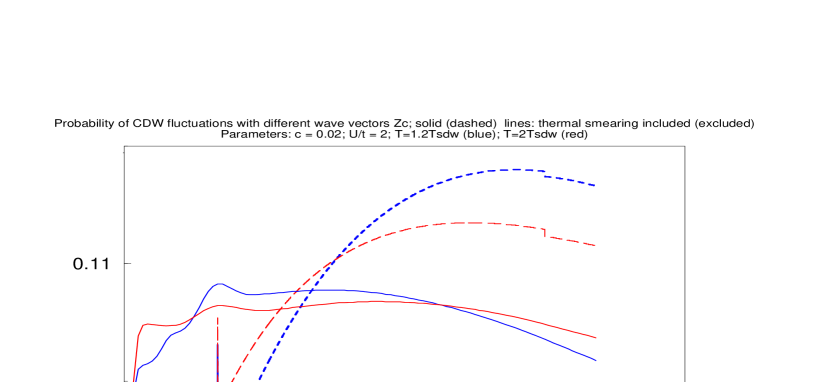
FIG. 1.:

 

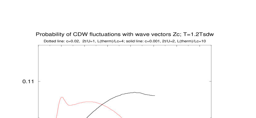
FIG. 2.:

 

FIG. 3.:

 

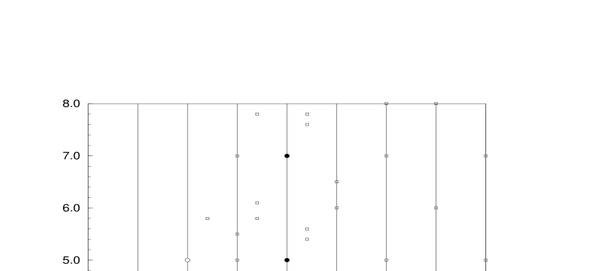
FIG. 4.:

 

FIG. 5.:

 

FIG. 6.:

 

FIG. 7.:

 

FIG. 8.:

 

FIG. 9.:

FIG. 10.: The qualitative phase diagram: the phase transition between stripe and antiferromagnet state is first order, other transition lines are second order. All three lines of phase transitions are intersected at the Lifshitz point P.

REFERENCES

- [1] S-W. Cheong et al., Phys. Rev. Lett. 67, 1791 (1991); J.M. Tranquada et al., Nature (London) 375, 561 (1995).
- [2] P. Dai et al., Science, 284, 1344 (1999); H. Kimura et al., Phys. Rev. B 59, 6517 (1999).
- [3] M. Fujita et al., Phys. Rev. B 65, 064505 (2002).
- [4] J. Zaanen and O. Gunnarson, Phys. Rev. B 40, 7391 (1989).
- [5] H.J. Schulz, J. Phys. (Paris) 50, 2833 (1989); Phys. Rev. Lett. 64, 1445 (1990); ibid. 65, 2462 (1990).
- [6] V.J. Emery, S.A. Kivelson, and H -Q. Lin, Phys. Rev. Lett. 64, 475 (1990); C. Castellani, C. Di Castro and M. Grilli, ibid. 75, 4650 (1995).
- [7] S.A. Kivelson, E. Fradkin, V.J. Emery, Nature 393, 550 (1998).
- [8] S.I.Mukhin, J. Phys. Chem. Solids 59, 1846 (1998).
- [9] S.I.Mukhin and Jan Zaanen, unpublished (1998).
- [10] S.I. Mukhin, Phys. Rev. B 62, 4332 (2000); cond-mat/9811409.
- [11] Yu.A. Bychkov, L.P. Gor’kov, and I.E. Dzyaloshinskii, Sov. Phys. JETP 23, 489 (1966).
- [12] I.E. Dzyaloshinskii and A.I. Larkin, Sov. Phys. JETP 34, 422 (1972); A.T. Zheleznyak, V.M. Yakovenko, and I.E. Dzyaloshinskii, Phys. Rev. B 55, 3200 (1997).
- [13] J. Solyom, Adv. Phys. 28, 201 (1979).
- [14] E.H. Lieb and F.Y. Wu, Phys. Rev. Lett. 20, 1445 (1968).
- [15] Jan Zaanen, private communications (2001).
- [16] S.I. Matveenko and S.I. Mukhin, Phys. Rev. Lett. 84, 6066 (2001).
- [17] S.A.Brazovskii, S.I.Matveenko, Sov. Phys. JETP 60, 804 (1984).
- [18] B. Horovitz, H. Gutfreund and M. Weger, Phys. Rev. B 12, 3174 (1975).
- [19] A.A. Abrikosov, L.P. Gor’kov and I.E. Dzyaloshinski, ”Methods of quantum field theory in statistical physics”, Dover Publications, N.Y. 1963, p. 130.
- [20] L.P. Gor’kov and A.G. Lebed’, J. Physique Lett. 45, L-433 (1984).
- [21] A. Erdelyi, W. Magnus, F. Oberhettinger and F.G. Tricomi, ”Higher transcendental functions”, New York-Toronto-London, 1953-1955.
- [22] M. Inui and P.B. Littlewood, Phys. Rev. B 44, 4415 (1991); J. Zaanen, P.B. Littlewood, Phys. Rev. B 50, 7222 (1994).
- [23] O. Zachar, S.A. Kivelson, and V.J. Emery, Phys.Rev. B 57, 1422 (1998).
- [24] L.V. Keldysh and Yu.V. Kopaev, Sov. Phys. Solid State 6, 2219 (1965).
- [25] L.P. Gor’kov and A.G. Lebed’, J. Physique Lett 45, L-433 (1984).
- [26] Formally, a leading harmonic approximation prevents one from keeping powers of with higher than 1 in the Bessel functions, but we use symbols to make more transparent derivation of Eq. (54) from Eq. (51).
- [27] K. Machida and M. Fujita, Phys. Rev. B 30, 5284 (1984).
- [28] Coupling constants and , characterizing Tc in the low- and high doping limits respectively, differ by factor , i.e. less than factor of 2 found for the Peierls model in S.A. Brazovskii, S.A. Gordyunin, and N.N. Kirova, JETP Lett. 31, 456 (1980). The discrepancy is satisfactory allowing for our few-harmonic aproximation.
- [29] Long-range Coulomb interaction would certainly influence the total energy balance of the stripe phase. This paper is focused on the major role of the on-site repulsion in the “selection” of the coupled SDW and CDW modes.
- [30] G. Grüner, Density Waves in Solids (Addison-Wesley, Reading, MA, 1994).
- [31] S.A.Brazovskii, JETP 78, 677 (1980); S. A.Brazovskii, S. A. Gordyunin, N. N. Kirova, JETP Lett. 31, 457 (1980).
- [32] W.P. Su, J.R. Schrieffer, and A.J. Heeger, Phys. Rev. Lett. 42, 1698 (1979); K. Machida and M. Fujita, Phys. Rev. B 30, 5284 (1984).
- [33] S. Brazovskii, N. Kirova, Sov. Sci. Rev A 6,99 (1984)
- [34] S.I.Matveenko, Sov. Phys. JETP 60, 1026 (1984).
- [35] I.E.Dzyaloshinskii, I.M.Krichever, JETP 56, 908 (1982).
- [36] A.I. Buzdin and V.V. Tugushev, Sov. Phys. JETP 85,428 (1984)
- [37] K. Machida and H. Nakanishi, Phys. Rev. B 30, 122 (1984).