Towards Noised-Induced Phase Transitions in Systems of Elements with Motivated Behavior

Abstract

A new type of noised-induced phase transitions that should occur in systems of elements with motivated behavior is considered. By way of an example, a simple oscillatory system $\{x,v=\dot{x}\}$ with additive white noise is analyzed numerically. A chain of such oscillators is also studied in brief.
PACS: 05.40.-a, 05.45.-a, 05.70.Fh
Keywords: motivated behavior, noise-induced phase transitions

1 Introduction

Systems of elements with motivated behavior (systems with motivation), e.g., fish and bird swarms, car ensembles on highways, stock markets, etc. often display noise-induced phase transitions (for a review see Ref. [3]). The ability of noise to induce phase transitions is now well established (see, e.g., Refs [1, 2]). However, in systems with motivation there is a special mechanism endowing the corresponding noise-induced phase transitions with distinctive properties.

For example, people as elements of a certain system cannot individually control all the governing parameters. Therefore one chooses a few crucial parameters and focuses on them the main attention. When the equilibrium with respect to these crucial parameters is attained the human activity slows down retarding, in turn, the system dynamics as a whole. For example, in driving a car the control over the relative velocity $v$ is of prime importance in comparison with the correction of the headway distance $x$. So, under normal conditions a driver should eliminate the relative velocity between her car and a car ahead first and only then correct the headway.

These speculations lead us to the concept of dynamical traps, a certain “low” dimensional region in the phase space where the main kinetic coefficients specifying the characteristic time scales of the system dynamics become sufficiently small in comparison with their values outside the trap region [4, 5]. The present paper analyzes the effect of noise on such a system and demonstrates that additive noise in a system with dynamical traps is able to give rise to new phases.

2 Noised oscillatory system with dynamical traps

By way of example, the following dimensionless system typically used to describe the oscillatory dynamics is considered:

$$\frac{dx}{dt}=v\,,\quad\frac{dv}{dt}=-\Omega(v)\left[x+\sigma v\right]+\epsilon\xi(t)\,,$$ (1)

where $\sigma$ is the damping decrement and the term $\epsilon\xi(t)$ is a random Langevin “force” of intensity $\epsilon$ proportional to the white noise $\xi(t)$ with unit amplitude. The function $\Omega(v)$ describes the dynamical trap effect arising in the vicinity of $v=0$. For this function, the following simple Ansatz

$$\Omega(v)=\frac{v^{2}+\triangle^{2}}{v^{2}+1}\,.$$ (2)

is used. In the chosen scales the thickness of the trap region is equal to unity and the parameter $\triangle\leq 1$ measures the trapping efficacy. When $\triangle=1$ the dynamical trap effect is ignorable, for $\triangle=0$ it is most effective.

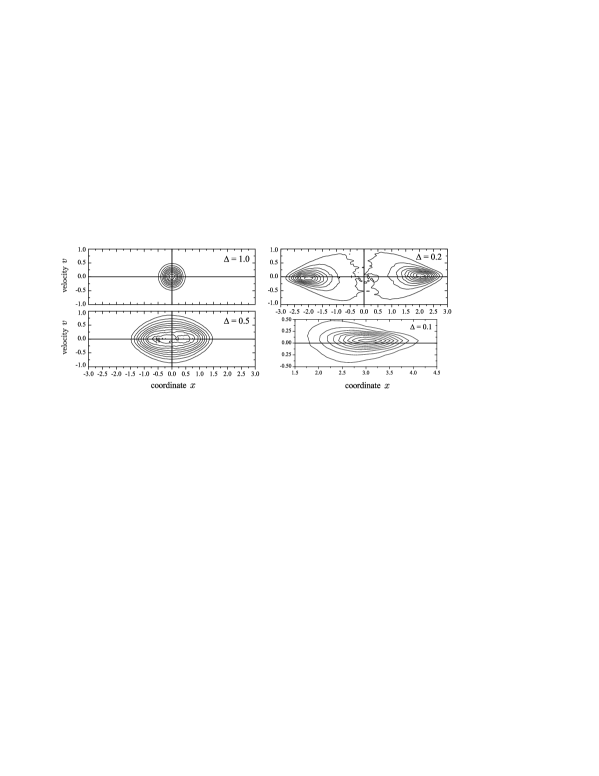
Figure 1: Evolution of the distribution function $\mathcal{P}(x,v)$ (shown by level contours) as the parameter $\triangle$ decreases. The parameters used are $\sigma=0.1$ and $\epsilon=0.1$. The lower right window depicts only one maximum of the distribution function.

System (1), (2) was analyzed numerically using the algorithm described in [6]. Figure 1 shows the distribution function $\mathcal{P}(x,v)$ of the system on the phase plane $\{x,v\}$, depending on the parameter $\triangle$. As can be seen this system undergoes a second order phase transition manifesting itself in the change of the shape of the phase space density $\mathcal{P}(x,v)$ from unimodal to bimodal as the trap parameter $\triangle$ decreases.

Mechanism of the phase transition

Figure 2 illustrates the mechanism of this phase transition. It depicts a typical fragment of the system motion through the trap region for $\triangle\ll 1$. When the path goes into the trap region $\mathcal{Q}_{t}$ ($|v|\ll 1$) the regular “force” $\Omega(v)(x+\sigma v)$ is depressed. So inside this region the system dynamics is mainly random due to the remaining weak Langevin “force” $\epsilon\xi(t)$. Crucial is the fact that the boundaries $\partial_{+}\mathcal{Q}_{t}$ (where $v\sim 1$) and $\partial_{-}\mathcal{Q}_{t}$ (where $v\sim-1$) are not identical in properties with respect to the system motion. At the boundary $\partial_{+}\mathcal{Q}_{t}$ the regular “force” leads the system inwards the trap region $\mathcal{Q}_{t}$, whereas at the boundary $\partial_{-}\mathcal{Q}_{t}$ it causes the system to leave the region $\mathcal{Q}_{t}$. Outside the trap region $\mathcal{Q}_{t}$ the regular “force” is dominant. Thereby, from the standpoint of the system motion inside the region $\mathcal{Q}_{t}$, the boundary $\partial_{+}\mathcal{Q}_{t}$ is “reflecting” whereas the boundary $\partial_{-}\mathcal{Q}_{t}$ is “absorbing”.

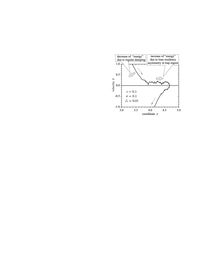
Figure 2: A typical fragment of the system path going through the trap region. The parameters $\sigma=0.1$, $\epsilon=0.1$, and $\triangle=0.01$ were used in numerical simulations in order to make the trap effect more pronounced.

As a result the distribution of the residence time at different points of the region $\mathcal{Q}_{t}$ should be asymmetric as shown in Fig. 1 (it is most clear in the lower right window). Therefore, during location inside the trap region the mean velocity must be positive, causing the system to go away from the origin. Outside the trap region the system motion is damping. So, when the former effect becomes sufficiently strong the distribution function $\mathcal{P}(\eta,u)$ becomes bimodal.

3 Chain of oscillators

A similar noise-induced phase transition for an ensemble of oscillators with dynamical traps is analyzed. The following one-dimensional model is considered, $N$ balls can move along $x$-axis interacting with the nearest neighbors, which is described by the equations for $i=1,2,\ldots N-1$

$$\frac{dx_{i}}{dt}=v_{i}\,,\quad\frac{dv_{i}}{dt}=-\Omega_{s}(v_{i-1},v_{i},v_{i+1})\left[\eta_{i}+\sigma\vartheta_{i}\right]+\epsilon\xi_{i}(t)\,.$$ (3)

Here $x_{i}$ is the coordinate of ball $i$, $v_{i}$ is its velocity, the variables $\eta_{i}$ and $\vartheta_{i}$ are given by the expression:

$$\eta_{i}=x_{i}-\tfrac{1}{2}(x_{i-1}+x_{i+1})\,,\quad\vartheta_{i}=v_{i}-\tfrac{1}{2}(v_{i-1}+v_{i+1})\,,$$ (4)

and $\{\xi_{i}(t)\}$ is the collection of white noise sources of unit amplitude and being mutually independent. The damping decrement $\sigma$ and the noise intensity $\epsilon$ are assumed to be the same for all the oscillators. The boundary balls ($i=0$ and $i=N$) are let to be fixed to prevent the ball system from moving as a whole. The function $\Omega_{s}(v_{i-1},v_{i},v_{i+1})$ measuring the trap effect due to the nearest neighbor interaction is given by the Ansatz

$$\Omega_{s}(v_{i-1},v_{i},v_{i+1})=\frac{(v_{i-1}-v_{i})^{2}+(v_{i}-v_{i+1})^{2}+\triangle^{2}}{(v_{i-1}-v_{i})^{2}+(v_{i}-v_{i+1})^{2}+1}\,,$$ (5)

where the parameter $\triangle$ has the same meaning as previously, it measures the intensity of trapping. The balls are assumed to be either mutually permeable or impermeable. In the latter case the absolutely elastic collision approximation is used.

The system of equations (3)–(5) was analyzed numerically. Below, the results are presented for the impermeable balls. Again integration of the stochastic differential equations was performed with the algorithms described in [6]. We analyzed an ensemble of 500 balls initially spaced 5 units apart and counted the number of balls falling into 100 identical intervals covering the system location region in the corresponding space.

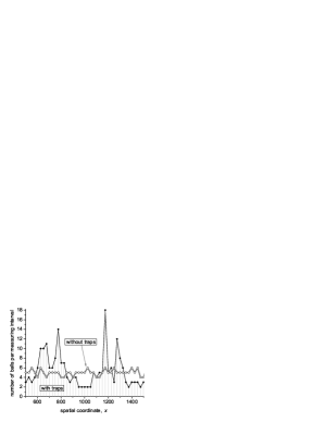
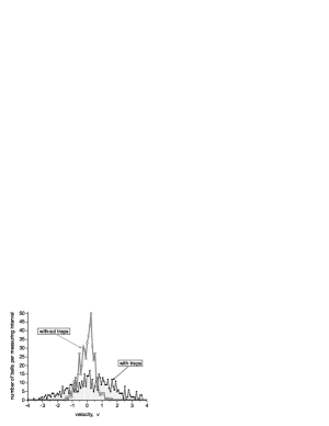
Figure 3: The ball distribution along the spatial axis and the velocity distribution at a fixed moment of time. These distributions are represented in terms of number of balls falling into measuring interval. The measuring intervals of number 100 cover the whole region of the system location in the corresponding space. The thick grey line and the boundary of dashed region match the cases where the trap effect is absent, $\triangle=1$, and strong, $\triangle=0.1$, respectively. The other parameters used are $\sigma=0.1$ and $\epsilon=0.1$.

Figure 3 actually depicts the ball distribution along the spatial axis and the velocity space at a fixed moment of time. As seen, the trap effect leads to the formation of a sufficiently inhomogeneous spatial distribution of balls whereas for the same system but without trapping, $\triangle=1$, the balls are actually uniformly distributed over the space region. In the velocity space the trap effect causes the balls to spread over a much wider domain.

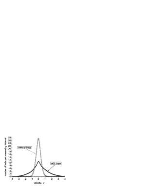
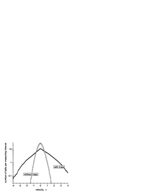
Figure 4: The time averaged velocity distribution presented in the same way as in Fig. 3. Here, however, the individual length of the measuring interval was decreased so their total number was 250. The parameters used are $\triangle=0.1$, $\sigma=0.1$ and $\epsilon=0.1$, the averaging time interval is 500 unit. The left and right windows depict the same data in linear and logarithmic scales, respectively.

To make the trap effect in the velocity space more clear we averaged the velocity distribution over 500 time units. The result is presented in Fig. 4. As seen, the strong trap effect causes a nonanalytic behavior of the velocity distribution at zero value, it takes the form of a cusp.

Finally, Fig. 5 illustrates the time pattern of the system dynamics. It is clear that the shown spatial structure is characterized by a long life time, because, we recall, the period of individual ball oscillations without traps is about $2\pi$.

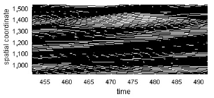
Figure 5: A fragment of the system time pattern. Black regions correspond to increased number of balls located in them.

4 Conclusion

A new type of noise-induced phase transitions in systems of elements with motivated behavior is considered. Dynamics of such systems, we think, should exhibit a number of anomalies due to dynamical traps. The dynamical traps form a low dimensional region in the phase space where the kinetic coefficients become sufficiently small and, as a result, the system spends a long time in it. The cause of the dynamical traps is, e.g., the inability of people or animals to control all the system governing parameters. So they have to focus the main attention on a few crucial ones and the intensity of their activity decreases when the system attains a local quasi-equilibrium with respect to these parameters.

To illustrate this effect a simple oscillatory system $\{x,v=\dot{x}\}$ is studied when the trap region is located in the vicinity of the $x$-axis and without noise the stationary point $\{x=0,v=0\}$ is absolutely stable. For this system as shown numerically an additive white noise can cause the phase-space density to take a bimodal shape. For the chain of such oscillators the trap effect gives rise to a substantially nonuniform spatial distribution and leads to nonanalytic behavior of the velocity distribution near zero value.

It should be underlined that a possible phase state that could be ascribed in this case to a maximum of the distribution function in the phase space does not match any stationary point of the “regular” or “random” forces.

References

- [1] W. Horsthemke and R. Lefever, Noise-Induced Transitions (Springer, Berlin, 1984).
- [2] Stochastic Dynamics, Lutz Schimansky-Geier and Thorsten Pöschel (eds.), Lecture Notes in Physics, Vol. 484 (Springer-Verlag, Berlin, 1998).
- [3] D. Helbing, Rev. Mod. Phys. 73, 1067 (2001).
- [4] I. Lubashevsky, R. Mahnke, P. Wagner, and S. Kalenkov, Phys. Rev. E 66, 016117 (2002).
- [5] I. Lubashevsky, M. Hajimahmoodzadeh, A. Katsnelson, and P. Wagner, e-print arXiv:cond-mat/0304300.
- [6] K. Burrage and P. M. Burrage, Appl. Numer. Math. 22, 81 (1996).