Soft modes in the easy plane pyrochlore antiferromagnet

Abstract

Thermal fluctuations lift the high ground state degeneracy of the classical nearest neighbour pyrochlore antiferromagnet, with easy plane anisotropy, giving a first order phase transition to a long range ordered state. We show, from spin wave analysis and numerical simulation, that even below this transition a continuous manifold of states, of dimension $N^{2/3}$ exist ($N$ is the number of degrees of freedom). As the temperature goes to zero a further ‘order by disorder’ selection is made from this manifold. The pyrochlore antiferromagnet Er₂Ti₂O₇, is believed to have an easy plane anisotropy and is reported to have the same magnetic structure. The latter is perhaps surprising, given that the dipole interaction lifts the degeneracy of the classical model in favour of a different structure. We interpret our results in the light of these facts.

In this paper we present a Monte Carlo study and classical spin wave analysis of an easy plane antiferromagnet on a pyrochlore lattice. The work was motivated by a recent comprehensive study of the rare earth pyrochlore Erbium titanate [1]. Er₂Ti₂O₇, which orders at 1.2 K [2] has been suggested to approximate the easy plane antiferromagnet [3, 4, 5]. We find that the magnetic structure of this simple model system is determined by an order by disorder mechanism [6] and that it is the same structure as that observed in the experiment.

The easy plane antiferromagnet

The pyrochlore lattice (see figure 2), has a rhombohedral primitive unit cell with lattice vectors,

$$\mathbf{a}=\left(\frac{1}{2}~{}\frac{1}{2}~{}0\right)\;,\mathbf{b}=\left(\frac{1}{2}~{}0~{}\frac{1}{2}\right)\;,\mathbf{c}=\left(0~{}\frac{1}{2}~{}\frac{1}{2}\right),$$

with a four atom basis at positions, $\mathbf{v}_{1}=0~{}0~{}0\;,\mathbf{v}_{2}=\frac{\mathbf{b}}{2}\;,\mathbf{v}_{3}=\frac{\mathbf{c}}{2}\;,\mathbf{v}_{4}=\frac{\mathbf{a}}{2}$, as shown in figure 2.

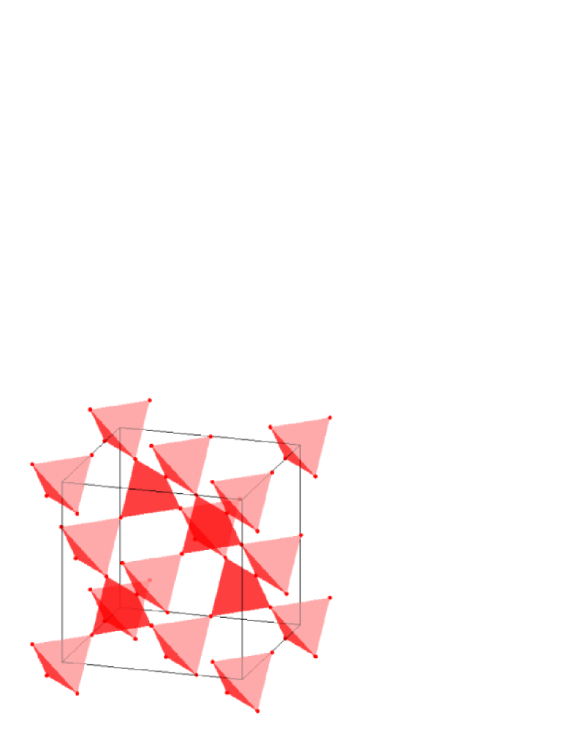
Figure 1: The pyrochlore lattice of corner-sharing tetrahedra

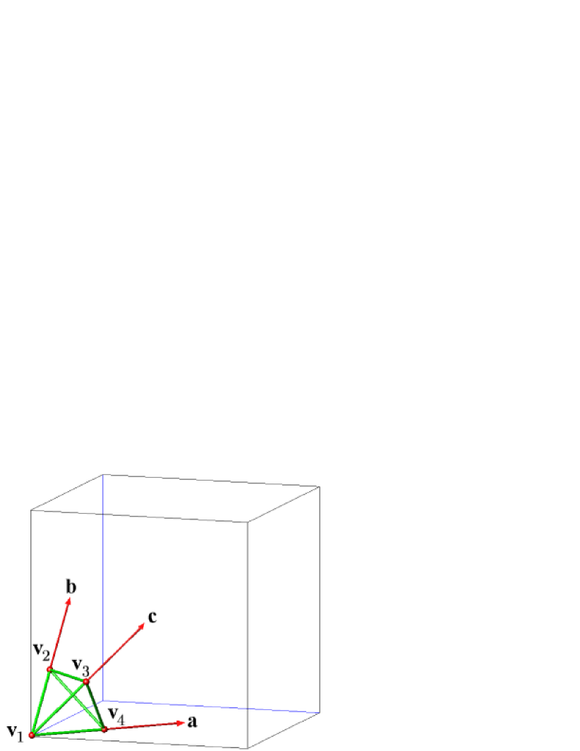
Figure 2: Rhombohedral axes with respect to the cubic unit cell

The units are those of a larger, cubic cell containing four tetrahedral cells [7]. The number of primitive cells, $N_{cell}=N/4$, where $N$ is the total number of spins and the linear dimension of the sample , $L=(N_{cell}/4)^{1/3}$.

We have studied the $D\rightarrow-\infty$ limit of the Hamiltonian

$$\mathbb{H}=-J\sum_{<i,j>}\mathbf{S}_{i}\cdot\mathbf{S}_{j}-D\sum_{i=1}^{N}\left(\boldsymbol{\delta}_{i}\cdot\mathbf{S}_{i}\right)^{2},$$

where $\boldsymbol{\delta}_{i}$ corresponds to a local $<111>$ anisotropy and the exchange constant $J=-1$. The spins are thus constrained to a plane oriented perpendicular to the local $<111>$ axis:

$$S_{x1}+S_{y1}+S_{z1}=0$$ (1a)

$$S_{x2}-S_{y2}+S_{z2}=0$$ (1b)

$$S_{x3}-S_{y3}-S_{z3}=0$$ (1c)

$$S_{x4}+S_{y4}-S_{z4}=0.$$ (1d)

The ground state condition for four antiferromagnetically coupled spins gives 3 further constraints [7]:

$$S_{x1}+S_{x2}+S_{x3}+S_{x4}=0$$ (1ba)

$$S_{y1}+S_{y2}+S_{y3}+S_{y4}=0$$ (1bb)

$$S_{z1}+S_{z2}+S_{z3}+S_{z4}=0.$$ (1bc)

In addition the spins are all of unit length:

$$|\mathbf{S}_{1}|=|\mathbf{S}_{2}|=|\mathbf{S}_{3}|=|\mathbf{S}_{4}|=1.$$ (1bc)

Linear equations (1a) – (1bc) can be solved by row-echelon matrix reduction [8]. The resulting dependent and independent variables are put into equation (1bc) to give four equations in terms of five variables. There is therefore one independent and continuous degree of freedom for four spins on a single tetrahedron in their ground state configuration. Full details of this solution can be found in Ref. [9].

The result for one tetrahedron suggests the possibility of a continuous ground state degeneracy when the tetrahedra are connected into a pyrochlore lattice and this is indeed what we found numerically, as shown below. This result is rather different from that found in Ref. [10], where the model was first studied. Here the authors only identify a discrete degeneracy and it was a surprise to find evidence of fluctuations over a continuous set of states.

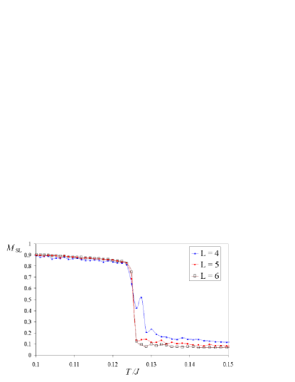
Figure 3: $M_{SL}$ vs $T/J$, showing a first order phase transition to an ordered q=0 state.

Monte Carlo simulations

Single spin-flip Monte Carlo simulations were performed on systems of size $N=432$ to $N=3456$, with periodic boundaries. The simulation lengths were typically $10^{5}$ moves per spin, with $40,000$ moves used for equilibration. As shown in figure 3, initial results confirm the strongly first order phase transition presented in Ref. [10]. The order parameter $M_{SL}$ is the sublattice magnetisation for each of the sites of the primitive cell, which we refer to as $q=0$ ordering. For $T\sim 0.125J$ the order parameter jumps from a small value characteristic of a finite system in a disordered phase to $M_{SL}\sim 0.85$, indicating an already highly ordered state.

Closer inspection [1] shows that the ground state chosen by the system is that shown in figure 4(a), not that proposed in Ref. [10] and shown in figure 4(b). The, initially proposed state has pairs of spins either aligned anti-parallel to each other or perpendicular to each other. We actually find scalar products between spins here of $-2/3$ and $1/3$. The spin components of both states are shown in Table 1.

(a) State 1

(b) State 2

Figure 4: Different ground states of the easy-plane tetrahedron antiferromagnet.

Table 1: The spin components of State 1 and State 2.

	State 1			State 2
i	$S_{x}$	$S_{y}$	$S_{z}$	$S_{x}$	$S_{y}$	$S_{z}$
1	$-\frac{1}{\sqrt{6}}$	$-\frac{1}{\sqrt{6}}$	$\frac{2}{\sqrt{6}}$	$\frac{-1}{\sqrt{2}}$	$\frac{1}{\sqrt{2}}$	0
2	$\frac{1}{\sqrt{6}}$	$-\frac{1}{\sqrt{6}}$	$-\frac{2}{\sqrt{6}}$	$-\frac{1}{\sqrt{2}}$	$-\frac{1}{\sqrt{2}}$	0
3	$-\frac{1}{\sqrt{6}}$	$\frac{1}{\sqrt{6}}$	$-\frac{2}{\sqrt{6}}$	$\frac{1}{\sqrt{2}}$	$\frac{1}{\sqrt{2}}$	0
4	$\frac{1}{\sqrt{6}}$	$\frac{1}{\sqrt{6}}$	$\frac{2}{\sqrt{6}}$	$\frac{1}{\sqrt{2}}$	$-\frac{1}{\sqrt{2}}$	0

It is easy to show that not all possible ground states have $q=0$ ordering. For example, in Ref. [10] O($L^{2}$) states were identified with spins ordered along one axis and with disorder in the planes perpendicular to this axis. The transition must therefore be driven by an order by disorder [6] mechanism, although no details of the entropic forces involved have previously been given. Below the transition it is clear that further entropic selection between different $q=0$ states must occur as we have already identified two different possibilities in figures 4(a) and 4(b), while the system systematically ends up in state 1 for $T\rightarrow 0$.

In figures 5(a), 5(b) and 5(c) we illustrate the evolution of this choice between different $q=0$ states. We show the distribution of nearest neighbour bond energies for three temperatures below the transition, for which, in all cases $M_{SL}>0.9$. For the highest temperature there is a continuous distribution of values from $-1$ (antiparallel spins) to $1/3$ where a sharp peak occurs. This figure is consistent with the result for a single tetrahedron, that a continuous degeneracy of $q=0$ ground states exists. One can see that going to the lowest temperatures the distribution slowly becomes peaked around energies $-2/3$ and $1/3$, corresponding to the ground state shown in figure 4(a). At all temperatures the energy is very close to the ground state energy and this figure clearly represents the order by disorder selection of a single point on a continuous energy surface. We expect the selection to be due to a singular excitation spectrum above the ground state at this point [11] and this is what we show in the next section.

\psfrag{P}{\huge{$P(E_{ij})$}}\psfrag{E}{\huge{$E_{ij}$}}\psfrag{0}{\huge$-1$}\psfrag{800}{\huge$~{}~{}1$}\psfrag{400}{\huge$~{}~{}0$}\psfrag{1}{\huge$0$}\includegraphics[angle={-90},width=110.96556pt]{fig_6.eps}

(a) $T/J=0.09$

\psfrag{P}{\huge{$P(E_{ij})$}}\psfrag{E}{\huge{$E_{ij}$}}\psfrag{0}{\huge$-1$}\psfrag{800}{\huge$~{}~{}1$}\psfrag{400}{\huge$~{}~{}0$}\psfrag{1}{\huge$0$}\includegraphics[angle={-90},width=110.96556pt]{fig_7.eps}

(b) $T/J=0.05$

\psfrag{P}{\huge{$P(E_{ij})$}}\psfrag{E}{\huge{$E_{ij}$}}\psfrag{0}{\huge$-1$}\psfrag{800}{\huge$~{}~{}1$}\psfrag{400}{\huge$~{}~{}0$}\psfrag{1}{\huge$0$}\includegraphics[angle={-90},width=110.96556pt]{fig_8.eps}

(c) $T/J=0.005$

Figure 5: Bond energy distributions $P(E_{ij})$ for various $T/J$.

Spin wave calculations

We consider small fluctuations out of the ground state 1. Working in the laboratory reference frame and re-defining ${}^{\alpha}\mathbf{S},\;\alpha=1,4$ as the spins in a given primitive cell, we make a small rotation, ${{}^{\alpha}S_{x}}={{}^{\alpha}S_{x0}}+{{}^{\alpha}\varepsilon}$ compatible with the local planar constraint. $S_{x0}$ is the ground state component and ${}^{\alpha}\varepsilon$ is the independent variable. ${}^{\alpha}S_{y}(^{\alpha}\varepsilon)$ and ${}^{\alpha}S_{z}(^{\alpha}\varepsilon)$ can thus be calculated by application of the constraints [9]. The Hamiltonian is then expanded to order $(^{\alpha}\varepsilon)^{2}$ and written in the form

$$\mathbb{H}-H_{o}=\frac{1}{2}\sum_{i}^{N_{cell}}\sum_{j}^{N_{cell}}\sum_{\alpha=1,\beta=1}^{\alpha=4,\beta=4}{{}^{\alpha}\varepsilon_{i}}\,\,\,M^{\alpha\beta}_{ij}\,\,\,{{{}^{\beta}}\varepsilon_{j}},$$ (1bd)

where $\alpha$ and $~{}\beta$ denote spins in a unit cell and $i$ and $j$ denote different unit cells (since all bonds are counted twice the sum is divided by 2). Note that due to the frustration, individual bonds make linear contributions in $(^{\alpha}\varepsilon)$, but as the ground state is a global minimum, these sum to zero. Once the dynamical matrix $M^{\alpha\beta}(\mathbf{R}_{ij})$ has been determined, it is Fourier transformed such that :

$$M^{\alpha\beta}(\mathbf{q})=\frac{1}{N_{cell}}\sum_{\mathbf{R}_{ij}}M^{\alpha\beta}(\mathbf{R}_{ij})\exp{(i\mathbf{q}.\mathbf{R}_{ij})},$$ (1be)

and (1bd) is reduced to

$$\mathbb{H}-H_{o}=\frac{1}{2}\frac{1}{N_{cell}}\sum_{\mathbf{q}}\sum_{\alpha\beta}{{}^{\alpha}\varepsilon_{\mathbf{q}}}\,\,M^{\alpha\beta}(\mathbf{q})\,\,{{}^{\beta}\varepsilon_{\mathbf{q}}},$$ (1bf)

where

$${{}^{\alpha}\varepsilon_{\mathbf{q}}}=\frac{1}{\sqrt{N_{cell}}}\sum_{\mathbf{R}_{i}}{{}^{\alpha}\varepsilon_{i}}\exp{(-i\mathbf{q}.\mathbf{R}_{i})}.$$ (1bg)

$M^{\alpha\beta}(\mathbf{q})$ is shown in matrix (1bh):

$$\left(\begin{array}[]{cccc}4J&0&0&2J\left(1+\rme^{\left(i\mathbf{q}.\mathbf{a}\right)}\right)\\ 0&4J&2J\left(1+\rme^{\left(i\mathbf{q}.\left(\mathbf{c}-\mathbf{b}\right)\right)}\right)&0\\ 0&2J\left(1+\rme^{\left(-i\mathbf{q}.\left(\mathbf{c}-\mathbf{b}\right)\right)}\right)&4J&0\\ 2J\left(1+\rme^{\left(-i\mathbf{q}.\mathbf{a}\right)}\right)&0&0&4J\\ \end{array}\right).$$ (1bh)

The eigenvalue equation, $f(\lambda)=0$ factorizes to the following form:

$$\left(\left(G-\lambda\right)^{2}-\frac{1}{2}G^{2}A\right)\left(\left(G-\lambda\right)^{2}-\frac{1}{2}G^{2}B\right)=0$$ (1bi)

where $G=4J$, $A=1+\cos(\mathbf{q}.\mathbf{a})$ and $B=1+\cos(\mathbf{q}.(\mathbf{c}-\mathbf{b}))$, giving

$$\lambda(\mathbf{q})_{\pm}=4J\left(1\pm\cos\left(\frac{\mathbf{q}.\mathbf{a}}{2}\right)\right)$$ (1bj)

$$\lambda(\mathbf{q})_{\pm}=4J\left(1\pm\cos\left(\frac{\mathbf{q}.(\mathbf{c}-\mathbf{b})}{2}\right)\right)$$ (1bk)

One can see that there are planes in reciprocal space perpendicular to $\mathbf{a}$ and to $(\mathbf{c}-\mathbf{b})$ for which $\lambda(\mathbf{q})=0$. We have verified that this is not the case for other selected $q=0$ ground states and it is these soft modes that provide the entropic force for the final ground state selection.

Using the mode counting arguments of Ref. [11] we can determine the effect of these zero modes on the specific heat. For a system with no soft modes, each degree of freedom will contribute $1/2$, in units of $k_{B}$ to the specific heat. In the harmonic approximation, the soft modes contribute zero. Assuming that this singularity is regularised at higher order by quartic corrections, each soft mode will contribute $(1/4)$.

One plane in reciprocal space contains $N_{cell}^{2/3}$ zero modes. The number of zero modes per unit cell is $2N_{cell}^{-1/3}$, since there are two planes. The specific heat per spin is thus:

$$\frac{C_{h}}{Nk_{B}T} = \frac{1}{4}\left[\left(4-2N_{cell}^{-1/3}\right)\frac{1}{2}+2N_{cell}^{-1/3}\frac{1}{4}\right]$$

$$= \frac{1}{2}-\frac{1}{8}\frac{1}{N_{cell}^{1/3}}$$

$$= \frac{1}{2}-\frac{1}{2^{11/3}}\frac{1}{L}$$

$$\frac{C_{h}}{Nk_{B}T} = \frac{1}{2}-C\frac{1}{L}$$ (1bl)

where $N_{cell}=4L^{3}$ and C is a constant. If $\frac{1}{2}-\frac{C_{h}}{N}$ is plotted versus $1/L$, a straight line graph should result. This figure has been tested by Monte Carlo (see figure 6). Data were collected for $L=1-7$ at a temperature of $T/J=0.0001$ with $1,000,000$ Monte Carlo steps per spin and $500,000$ equilibration steps, with five separate simulations averaged for each lattice point. There is good agreement with a linear fit, suggesting that our order by disorder scenario is correct. However the gradient, while it is the correct order of magnitude, is not correct: $0.063$ as opposed to the predicted value $0.0787$. We have not, at present been able to explain this discrepancy. Note that the entropic contribution to the free energy coming from the soft modes scales as $N^{2/3}$ and is therefore not extensive. This could mean that the ordering within the $q=0$ manifold occurs at a system size dependent temperature that goes to zero in the thermodynamic limit and the discrepancy could come from this effect; although the temperature here is very low. More work is required to resolve this point.

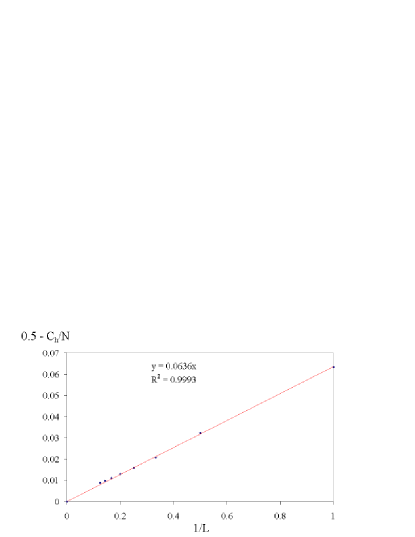
Figure 6: $\frac{1}{2}-\frac{C_{h}}{N}$ vs $\frac{1}{L}$ for State 1.

Conclusion

In this paper we have reported another example of order by disorder in a geometrically frustrated magnetic system (see for example [11, 12, 13]). We have exposed one order by disorder mechanism leading to the low temperature selection of an ordered state, but there are several interesting statistical mechanics questions that remain open: firstly, is there a different, perhaps discrete mechanism, analogous to that in Villain’s original paper [6], that drives the phase transition, or are the soft modes felt by the system, even in the disordered phase? Secondly, are there disordered states with the same soft mode structure? This is the case for the Heisenberg antiferromagnet on the kagomé lattice [11, 13] and the results here suggest that columnar line defects could exist, equivalent to the line defects of the kagomé lattice. It would be interesting to pursue this question further.

The project, in this case was strongly motivated by experimental results on Er₂Ti₂O₇ and its real interest lies in the question: is it in fact relevant? There are several details that the simple model does not correctly predict; most notably, experimentally the transition is second order [1] while here we find a very strongly first order transition. Further, experimentally the low temperature specific heat varies like $T^{3}$ [1], which is indicative of a spin wave spectrum with a quadratic density of energetic states. We have calculated the density of eigenvalues above the zero frequency modes and find $g(\lambda)=const.$, which is compatible with having degenerate planes in reciprocal space and variations along only one dimension. Here, of course, we cannot capture the quantum fluctuations as our model only has one degree of freedom per spin. To study this question more closely one would need to add out of plane fluctuations, although it is difficult to see how this could lead to a quadratic density of states. It might be interesting to look at this problem in the future. However, despite these failings our simple model does have one great success: it does predict the correct magnetic structure for Er₂Ti₂O₇ [1]. This seems particularly interesting considering that dipolar corrections, which one might expect to be the most substantial perturbation [14] would lead to a different magnetic structure [15]. A classical model, with dipoles would predict the ground state shown in figure 4(b), which is different from the experimentally observed structure. With this result we suggest that our model is a relevant starting point to study this compound and it will be interesting to see if quantum fluctuations can change the details discussed above.

References

References

- [1] Champion J D M et al2003 Phys. Rev. B 68 020401(R)
- [2] Blöte H W J et al 1969 Physica 43 549
- [3] Rosenkranz S et al 2000 J. Appl. Phys. 87 5914
- [4] Siddharthan R et al 1999 Phys. Rev. Lett. 83 1854
- [5] Harris M J et al 1998 J. Magn. Magn. Mater. 177 757
- [6] Villain J 1980 J. Physique 41 1263
- [7] Reimers J N, Berlinsky A J and Shi A C 1991 Phys. Rev. B 43 865
- [8] Boas M L 1983 Mathematical Methods in the Physical Sciences (New York, Chichester: Wiley)
- [9] Champion J D M 2001 Ph.D. Thesis, University of London
- [10] Bramwell S T, Gingras M J P and Reimers J N 1994 J. Appl. Phys. 75 5523
- [11] Chalker J T, Holdsworth P C W and Shender E F 1992 Phys. Rev. Lett. 68 855
- [12] Moessner R and Chalker J T 1998 Phys. Rev. Lett. 80 2929
- [13] Zhitomirsky M E 2002 Phys. Rev. Lett. 87 057204
- [14] Bramwell S T and Gingras M J P 2001 Science 294 1495
- [15] Palmer S E and Chalker J T 2000 Phys. Rev. B 62, 488