Fluid-like behavior of a one-dimensional granular gas

Abstract

We study the properties of a one-dimensional (1D) granular gas consisting of $N$ hard rods on a line of length $L$ (with periodic boundary conditions). The particles collide inelastically and are fluidized by a heat bath at temperature $T_{b}$ and viscosity $\gamma$. The analysis is supported by molecular dynamics simulations. The average properties of the system are first discussed, focusing on the relations between granular temperature $T_{g}=m\langle v^{2}\rangle$, kinetic pressure and density $\rho=N/L$. Thereafter, we consider the fluctuations around the average behavior obtaining a slightly non-Gaussian behavior of the velocity distributions and a spatially correlated velocity field; the density field displays clustering: this is reflected in the structure factor which has a peak in the $k\sim 0$ region suggesting an analogy between inelastic hard core interactions and an effective attractive potential. Finally, we study the transport properties, showing the typical sub-diffusive behavior of 1D stochastically driven systems, i.e. $\langle|x(t)-x(0)|^{2}\rangle\sim Dt^{1/2}$ where $D$ for the inelastic fluid is larger than the elastic case. This is directly related to the peak of the structure factor at small wave-vectors.

I Introduction

Scientists and engineers have been studying granular materials for nearly two centuries for their relevance both in natural processes (landslides, dunes, Saturn rings) and in industry (handling of cereals and minerals, fabrication of pharmaceuticals etc.). general1 ; general2 ; general3 ; general4 The understanding of the “granular state” still represents an open challenge and one of the most active research topics in non-equilibrium statistical mechanics and fluid dynamics. For instance, a way to attack the problem consists in fluidizing the grains by shaking them so that the system behaves as a non-ideal gas, a problem relatively easier to study. The difficulty, but also the beauty, of the dynamics of granular gases, meant as rarefied assemblies of macroscopic particles, stems from the inelastic nature of their collisions which leads to a variety of very peculiar phenomena. Several theoretical methods have been employed to deal with granular gases ranging from hydrodynamic equations, kinetic theories to molecular dynamics. Engineers often prefer the strategy of the continuum description because it gives a better grasp of real life phenomena, while natural scientists tend to opt for a microscopic approach, to better control each step of the modelization. The latter, as far as the interaction between particles is concerned, regards granular systems as peculiar fluids, and treats them through the same methods which have been successfully applied to ordinary fluids. hansen This allows not only, to employ concepts already developed by physicists and chemists, but also to stress analogies and substantial differences.

The purpose of the present paper is to establish such a connection for a system of stochastically driven inelastic hard-rods constrained to move on a ring. The elastic version of this system has a long tradition lord ; tonks ; takahashi ; frenkel ; gursey ; salsburg ; percus and is particularly suitable to test approximations and theories since many of its equilibrium properties can be derived in a closed analytical form. Even though, the one dimensional geometry introduces some peculiarities not shared by real fluids, we shall show that the model provides many useful information and a very rich phenomenology which closely recalls the behavior of microscopic particles confined in tubules or cylindrical pores with little interconnection. A second reason to investigate such a model is to show how the inelasticity of interactions influences not only the average global properties of a system, but also its microscopic local structure.

A basic requirement to a theoretical description of a granular gas is to provide an equation of state linking the relevant control parameters and possibly to relate it to the microscopic structure of the system. This connection is well known for classical fluids, where thermodynamic and transport properties are linked to the microscopic level via the correlation function formalism.

One dimensional models have been employed by several authors as simple models of granular gases. mcnamara ; sela ; grossman ; zhou ; zhou2 ; kadanoff ; mackintosh ; puglisi ; puglisi2 ; bennaim ; cordero ; baldassarri The differences between the various models stem chiefly from the choice of the thermalizing device. In fact, granular gases would come to rest unless supplying energy compensating the losses due to the inelastic collisions. We call, by analogy, “heat bath” the external driving mechanism maintaining the system in a statistically steady state.

For the history, the first 1D models, which were proposed, had no periodic boundary conditions and the energy was injected by a vibrating wall (stochastic or not). This kind of external driving however, was not able to keep the system homogeneous, because only the first and last particle had a direct interaction with the wall. kadanoff As an alternative, a uniform heating mechanism, namely a Gaussian white noise acting on each particle, was introduced. mackintosh Later Puglisi et al.puglisi added a second ingredient, consisting of a friction term that prevents the kinetic energy from diverging. With such a modification the system reaches a steady regime and time averages can be safely computed. In the present paper we shall focus on this last model characterizing its steady state properties.

The layout is the following: in section II we introduce the model, in section III we obtain numerically and by approximate analytical arguments equations for the average kinetic energy and pressure. Section IV is devoted to fluctuations of the system observables around their average values. In section V we study the diffusion properties of the system. Finally, in section VI we present the conclusions.

II The model

Inelastic hard sphere models are perhaps the simplest models able to capture the two salient features of granular fluids, namely the hard core repulsion between grains and the dissipation of kinetic energy due to the inelastic collisions. Since many of the equilibrium properties of the 1D elastic hard rods are known in closed analytical form, such a system represents an excellent reference model even for the inelastic case. Let us consider $N$ identical impenetrable rods, of coordinates $x_{i}(t)$, mass $m$ and size $\sigma$, constrained to move along a line of length $L$. Periodic boundary conditions are assumed. The hard-core character of the repulsive forces among particles reduces the interactions to single binary, instantaneous collision events occurring whenever two consecutive rods reach a distance $d_{i}(t)=x_{i}(t)-x_{i-1}(t)$ equal to their length $\sigma$. When two inelastic hard-rods collide, their post-collisional velocities (primed symbols) are related to pre-collisional velocities (unprimed symbols) through the rule:

$$v_{i}^{\prime}=v_{i}-\frac{1+r}{2}(v_{i}-v_{j})$$ (1)

where $r$ indicates the coefficient of restitution. The interaction of each particle with the heat-bath is represented by the combination of a viscous force proportional to the velocity and a stochastic force. Then each particle follows the so called Kramers dynamics

$$\frac{dx_{i}}{dt} = v_{i}$$ (2)

$$m\frac{dv_{i}}{dt} = -m\gamma v_{i}+\xi_{i}(t)$$ (3)

where $\gamma$ is the viscous friction coefficient, $\xi_{i}(t)$ is a Gaussian white noise with zero average and correlation

$$\langle\xi_{i}(t)\xi_{j}(s)\rangle=2\gamma mT_{b}\delta_{ij}\delta(t-s)\;,$$ (4)

$T_{b}$ is the “heat-bath temperature” and $\langle\cdot\rangle$ indicates the average over a statistical ensemble of noise realizations.

We have developed a numerical simulation code for hard rods interacting through momentum conserving but energy dissipating collisions. In our simulations the motion between two consecutive collisions is governed by the dynamics (2,3). Thus, we determine the instant when the first collision among the $N$ particles occurs and change their velocities and positions according to the equations of motion. The effect of the collision is taken into account by updating the velocities after each collision according to the rule (1).

We tested our code on the elastic case ($r=1$) and checked that our simulations faithfully reproduced the well known properties of the equilibrium hard rod system.

III Average properties

We begin by considering the steady state properties of the model. The aim is to derive relations connecting the microscopic parameters to the “thermodynamic” observables such as temperature and pressure and eventually to obtain an “equation of state” relating these two quantities. In order to achieve this goal we assume that the system is homogeneous, so that its density $\rho$ is constant.

III.1 Kinetic temperature

Collisions and the Kramers’ dynamics entail that the time derivative of the average kinetic energy per particle is

$$\frac{d}{dt}\frac{1}{2}m\langle v(t)^{2}\rangle=\gamma(T_{b}-T_{g})-w(t),$$ (5)

where $T_{g}=m\sum_{i=1}^{N}v_{i}^{2}/N$ is the granular temperature and $w(t)$ is the average power dissipated by collisions, given by $w=\frac{1-r^{2}}{8}m\langle\delta v^{2}\rangle/\tau_{c}$, where $\delta v$ is the difference between the pre-collisional velocities of the colliding pair. The average collision time $\tau_{c}$ is estimated by assuming a mean free path $\lambda=(L-\sigma N)/N$, where $L-\sigma N$ is the free volume. We obtain, in terms of the system density $\rho=N/L$,

$$\tau_{c}=\frac{\lambda}{v}=\frac{1-\sigma\rho}{\rho}\sqrt{\frac{m}{T_{g}}}.$$ (6)

Thus the average power dissipated per grain reads:

$$w=\frac{1-r^{2}}{8}\langle\delta v^{2}\rangle\frac{\rho\sqrt{T_{g}m}}{1-\sigma\rho}.$$ (7)

In order to estimate $T_{g}$ we assume that $m\langle\delta v^{2}\rangle\simeq 4T_{g}$ since the velocities of the colliding pairs are strongly correlated. Thus imposing the solution of Eq. (5) to be stationary we obtain for $T_{g}$ the following expression:

$$T_{g}=\frac{T_{b}}{1+\frac{1-r^{2}}{2\gamma}\frac{\rho}{1-\rho\sigma}\sqrt{\frac{T_{g}}{m}}}.$$ (8)

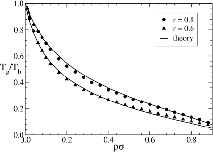
Figure 1: Comparison between the numerical results for the granular temperature versus density and the corresponding theoretical expression Eq. (8). The simulation data refer to $\sigma=0.2$, $\gamma=0.2$, $T_{b}=1.0$, $r=0.6$ and $r=0.8$. We kept the system size fixed to $L=40$ but varied the number of particles $N$ to change the density.

In figure 1 we compare formula (8) with the results of numerical simulations at various densities. In spite of the simplicity of the argument used to derive Eq. (8), the agreement between $T_{g}$ extracted by simulations and its theoretical estimate is fairly good.

III.2 Kinetic pressure

In a granular system the total pressure, $P$, can be obtained via its mechanical or kinetic definition, i.e. as the impulse transferred across a surface in the unit of time.allen ; barrat The pressure contains both the ideal gas and the collisional contribution ($P_{id}$ and $P_{exc}$ respectively)

$$P=P_{id}+P_{exc}=\rho T_{g}(\rho)+\frac{\sigma}{Lt_{ob}}\sum_{k=1}^{M_{c}}\delta p_{k}$$ (9)

where the second equality stems from the virial theorem. erpenbeck Here $t_{ob}$ is the observation time, the sum runs over the $M_{c}$ collisions and $\delta p_{k}=m\delta v_{k}$ represents the impulse variation due to the $k$-th collision.

An approximate formula for $P_{exc}$ can be derived as follows. The average collision frequency per particle can be estimated as $\tau_{c}^{-1}=(M_{c}/t_{ob})/N$. By replacing in Eq. (9) $t_{ob}$ with $(M_{c}/N)\tau_{c}$ and using $\tau_{c}$ given by Eq. (6), we obtain, for the excess part of the pressure, the expression

$$P_{exc}=\frac{N\sigma}{\tau_{c}L}m\langle\delta v_{c}\rangle=\frac{\rho^{2}\sigma}{1-\sigma\rho}T_{g}(\rho).$$ (10)

Collecting pieces together we arrive at

$$P(\rho)=T_{g}(\rho)\bigg{[}\rho+\frac{\sigma\rho^{2}}{1-\sigma\rho}\bigg{]}\;=\;T_{g}(\rho)\frac{\rho}{1-\sigma\rho}$$ (11)

which reproduces the well known Tonks formula tonks in the case of elastic particles and constitutes the sought equation of state for the inelastic system. Let us recall that in the elastic case, Eq. (11) can be written in the virial form

$$P(\rho)=T_{g}(\rho)\rho[1+\rho\sigma g(\sigma)]$$ (12)

showing the connection between the macroscopic and the microscopic level, since $g(\sigma)=1/(1-\rho\sigma)$ is the equilibrium pair correlation at contact.

We see, from figure (2), that the presence of the prefactor $T_{g}(\rho)$, which is decreasing function of the density, makes $P(\rho)$ to increase more slowly than the corresponding pressure of the elastic system in the same physical conditions (i.e. same density and contact with the same heat bath).

Equations (8) and (10) for temperature and pressure coincide, in the limit $\gamma\to 0$, $\sigma\to 0$, $\gamma T_{b}=\Omega=\mbox{const}$, with those derived by Williams and MacKintosh mackintosh .

Following the standard approach to fluids, we define, even for the inelastic system, the response of the density to a uniform change of the pressure for a fixed value of the heat bath temperature:

$$\chi_{T}=\frac{1}{\rho}\frac{\partial\rho}{\partial P}$$ (13)

which is plotted in figure 3. We observe that the response of the inelastic system to a compression is much larger than the corresponding elastic system at the same density, due to the tendency to cluster.

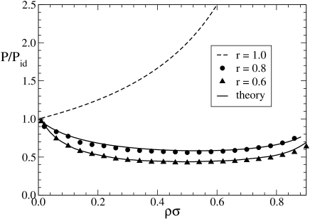
Figure 2: Comparison between the kinetic pressure obtained from the simulations and the prediction of Eq. 11 at different densities for inelastic hard rods with coefficients of restitution $r=0.6$ and $r=0.8$. The remaining parameters are the same as in figure 1. Dashed line refers to the pressure of the corresponding elastic system.

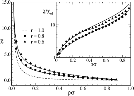
Figure 3: Compressibility, computed from Eq. (13), plotted versus density, for inelastic hard rods with coefficient $r=0.6$ (the remaining parameters are the same as in figure 1). Symbols refers to simulations while solid lines are the theoretical predictions obtained via the expression for the pressure (11). The curve for the elastic system $r=1$ (dashed line) is also reported for sake of comparison. In the inset shows the ratio between the inelastic and elastic compressibility.

IV Fluctuations

So far we have considered only the global average properties of the granular gas. It is well known, on the other hand, that these system may exhibit strong spontaneous deviations from their uniform state. In this section we shall study fluctuations of the main observables in order to understand the qualitative effect of inelasticity on such a peculiar fluid.

IV.1 Velocity distributions

One of the signatures of the inelasticity of the collisions is represented by the shape of the velocity distribution function (VDF), $P(v)$. Non-Gaussian VDF’s, displaying low velocity and high velocity overpopulated regions, have been measured experimentally losert ; menon ; Blair ; urbach ; aranson ; kudrolli and in numerical simulations.puglisi ; breyvel In figure 4 we show two VDF corresponding to two different values of $r$.

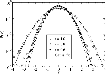
Figure 4: Velocity distributions $P(v)$ for three values of the coefficient of restitution $r=1.0$ (circles), $0.8$ (squares), $0.6$ (triangles). The remaining parameters are $N=1000$, $L=1000$, $\sigma=0.2$, $T_{b}=1.0$, $\gamma=0.2$. Dashed lines indicates the corresponding Gaussian fit.

Theoretical, numerical and experimental studies have shown that the VDF for inelastic ($r<1$) gases usually displays overpopulated tails. The literature seems to indicate the lack of a universal VDF: in $d>1$ the solution of the homogeneous Boltzmann equation with inelastic collisions (with a stochastic driving similar to ours but without viscosity) has overpopulated tails of the kind $\sim\exp(-v^{3/2})$.ernst

IV.2 Energy fluctuations

Interestingly, the energy fluctuations of our system, $E\equiv m\sum_{i}v_{i}^{2}$/2, display a scaling with respect to the number of particles. We are interested in the quantity $({\langle E^{2}\rangle-\langle E\rangle^{2})/\langle E\rangle^{2}}$ as a function of $N$ (at fixed density $\rho$). Defining $\langle v^{n}\rangle=\int v^{n}P(v)dv$, we have

$$\langle E^{2}\rangle-\langle E\rangle^{2}=\frac{m^{2}}{4}\sum_{i,j}\bigg{(}\langle v_{i}^{2}v_{j}^{2}\rangle-\langle v_{i}^{2}\rangle\langle v_{i}^{2}\rangle\bigg{)}$$ (14)

Under the hypothesis that the variables $v_{i}$ are independently distributed, we get

$$\langle E^{2}\rangle-\langle E\rangle^{2}=\frac{m^{2}}{4}{[N\langle v^{4}\rangle-N\langle v^{2}\rangle^{2}]}$$ (15)

Since for Gaussian variables $\langle v^{4}\rangle=3\langle v^{2}\rangle^{2}$, we find

$$\frac{\langle E^{2}\rangle-\langle E\rangle^{2}}{\langle E\rangle^{2}}=\frac{2}{N}$$ (16)

which is a well known formula for equilibrium systems huang . This scaling is fairly well verified in figure 5.

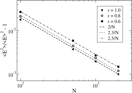
Figure 5: Energy fluctuation as a function of the number of particles, $N$ for $r=1.0,0.8,0.6$. The elastic case agrees with the theoretical prediction $2/N$, whereas the inelastic case gives a value of the relative fluctuation slightly larger. The remaining parameters are the same as in figure 4

In the case of a granular fluid, $P(v_{i})$ is no more Gaussian, exhibiting fatter tails, so one observes $\langle v^{4}\rangle\geq 3\langle v^{2}\rangle^{2}$ (for example in the case $r=0.6$ we have $\langle v^{4}\rangle/\langle v^{2}\rangle\approx 3.3$). This leads to the conclusion that the scaling $\sim 1/N$ of formula (16) still holds, but with a coefficient larger than $2$. Simulation runs for $r=0.6$ confirm this prediction (Fig. 5). The renormalization of the multiplicative constant occurring in the inelastic system could be interpreted also as an “effective reduction” of the number of degrees of freedom. Indeed, the inelastic system has the tendency to cluster, as it will be shown, and therefore the effective number of independent “particles” appears smaller. Another appealing interpretation is that the inelastic systems possesses an effective “specific heat” larger than that of elastic systems.

IV.3 Velocity correlations

A universal signature of the inelasticity is the presence of correlations between the velocities of the particles. We measured the structure function of the velocities $v_{i}$, $S_{v}(k)=\langle\tilde{v}(k)\tilde{v}(-k)\rangle$, where $\tilde{v}(k)$ is the Fourier transform of $v_{i}$. In figure 6, we show three $S_{v}(k)$ corresponding to the elastic ($r=1$) and inelastic system with $r=0.8$ and $r=0.6$.

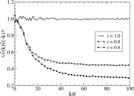
Figure 6: Structure function of the velocity field $v_{i}$, for elastic and inelastic systems. The control parameters are the same as in figure 4

As mentioned above, the elastic systems is characterized by uncorrelated velocities and this reflects on a constant structure function. A certain degree of correlation is instead evident in the inelastic system. In fact, the inelasticity reduces by a factor $r$ the relative velocity of two colliding particles and this leads to an increasing correlation among velocities. However, the noise induced by the bath competes with these correlations, making the structure function not very steep. More specifically, $S_{v}(k)$ can be fitted, in the middle range of $k$ values, by an inverse power $\sim k^{-0.5}$, while at high $k$ values it reaches a constant plateau. This is the fingerprint of a persistent internal noise (velocity fluctuations are not completely frozen by inelastic collisions).Ernstprogram

IV.4 Distribution of interparticle spacing and of collision times

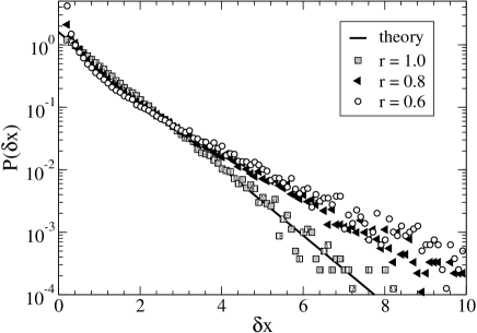
Figure 7: Distributions of distances between nearest neighbor particles $\delta x=x_{i}-x_{i-1}$, for elastic and inelastic systems, with the same parameters used before. The solid line indicates the exponential expected in the elastic case (see text). The state parameters are the same as in Fig. 4

The probability distribution, $P(\delta x)$, of distances between nearest neighbor particles $\delta x=x_{i}-x_{i-1}$, shown in figure 7, provides information about the spatial arrangement of the system. In the elastic case one easily finds

$$P(\delta x)=\frac{1}{\lambda}\exp[-(\delta x-\sigma)/\lambda]$$ (17)

for $\delta x\geq\sigma$ and $0$ for $\delta x<\sigma$ with $\lambda=(1-\rho\sigma)/\rho$. The presence of inelasticity modifies such a simple exponential law in the way shown in figure 7. In this case, the probability of finding two particles at small separation increases together with that of finding large voids. Such a picture is consistent with the idea of the clustering phenomenon:zanetti two particles, after the inelastic collision, have a smaller relative velocity and therefore reach smaller distances, eventually producing dense clusters and leaving larger empty regions with respect to the elastic case.

On the contrary, the probability distribution of collision times, shown in figure 8, appears to always follow the theoretical (elastic) form $P(t)=1/\tau_{c}\exp(-t/\tau_{c})$. Apart from a trivial rescaling due to the change of the thermal velocity with $r$, it seems not to depend appreciably on the coefficient of restitution.

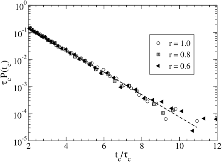
Figure 8: Distributions of collision times. The dashed line indicates the exponential law expected for the elastic system (see text). Control parameters as in figure 7.

Such a finding is in contrast with the situation observed in 2D vibrated granular systems Paolotti ; Blair . A possible explanation for this discrepancy is the following: in the inelastic 1D system, there is correlation between the relative velocities and the free-paths (or free-times), otherwise the distribution $P(t)$ and $P(\delta x)$ would have had the same shape due to the trivial relation $x=vt$, $v$ being the the average velocity of the rods. In particular, the fact that the peak of $P(\delta x)$ in $\delta x=0$ does not yield a corresponding peak in the $t=0$ region of $P(t)$ suggests that the shorter the distance between particles the smaller their relative velocity.

IV.5 Density fluctuations

We turn, now, to the study of the structural properties of the inelastic hard-rod gas, by considering the pair correlation function or the structure factor. As mentioned in section II, the virial equation (12) relates the pressure of an elastic hard-rod system to its microscopic structure. In the presence of inelasticity, however, we expect that the tendency to cluster is mirrored by a change in the structural properties of the fluid. Therefore we considered the behavior of the static (truly speaking steady state) structure factor

$$S(k)=1+\rho\int dx[g(x)-1]e^{ikx}$$ (18)

for different values of $\rho\sigma$ and inelasticity.

The spatial structure of the system is determined, as in ordinary fluids, by the strong repulsive forces. Their role is seen in the oscillating structure of $g(x)$. The inelastic nature of the collisions provides a correction to $g(x)$, which can be better appreciated by studying the small wavelength behavior of $S(k)$ which develops a peak at small $k$ recalling the Ornstein-Zernike behavior

$$S(k)\simeq\frac{1}{S^{-1}(0)+c_{2}k^{2}}\;.$$ (19)

The coefficient $c_{2}$ is negative for hard rods, whereas it is positive for the inelastic system. For hard rods, $S(k)$ is known percus and reads:

$$S(k)=\frac{1}{1+2b\rho\sigma\frac{\sin(k\sigma)}{k\sigma}+(b\rho\sigma)^{2}\frac{\sin^{2}(k\sigma/2)}{(k\sigma/2)^{2}}}$$ (20)

with $b=\frac{1}{1-\rho\sigma}$.

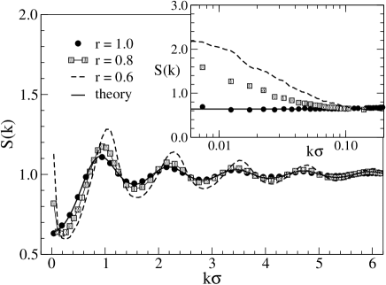
Figure 9: Typical behavior of the structure function of $S(k)$ for different values of the coefficients $r=1.0,0.8,0.6$. Notice the growth of the peak at small $k$ when $r$ decreases.

Figure 9 shows the typical behaviors of $S(k)$ for elastic and inelastic systems. The numerically computed structure factor of the elastic system agrees rather well with equation (20). The inelastic system, instead, displays a peak in the small $k$ region reflecting the tendency of the fluid to cluster. The peak increases with inelasticity, demonstrating that the energy dissipation in collisions is responsible for these long range correlations. Incidentally, we comment that such a behavior of $S(k)$ could be attributed to the presence of a long range attractive effective potential between the rods, as a result of dynamical correlations.ernst2

MackIntosh and Williams mackintosh found that, in the case of randomly kicked rods in the absence of viscosity, the pair correlation function decays as an inverse power law, $g(x)\propto x^{-\eta}$ with $\eta\to 0$ for $r\to 1$ and $\eta\to 1/2$ for $r\to 0$. Correspondingly, one expects $S(k)$ to diverge as $k^{-1/2}$ as $k\to 0$, for very inelastic systems. In other words, the inelasticity leads to long range spatial correlations which are revealed by the peak at small $k$ of $S(k)$. We remark that, in spite of the apparent similarity between the equations of state for elastic and inelastic system, their structural properties are radically different. Such a phenomenon is the result of the coupling of the long-wavelength modes of the velocity field with the stochastic non-conserved driving force. In fact, due to the inelastic collisions, the velocities of the particles tend to align, thus reducing the energy dissipation. On the other hand, these modes adsorb energy from the heat bath and grow in amplitude, and only the presence of friction prevents these excitations from becoming unstable. The density field, which is coupled to the velocity field by the continuity equation, also develops long range correlations, and the structure factor displays a peak at small wave-vectors.

V Transport properties

One dimensional hard-core fluids exhibit an interesting connection between the microscopic structural properties and diffusive ones. In the present section, we present numerical results for the collective diffusion and for the diffusion of a tagged particle and show how these are connected to the structure.

V.1 Collective Diffusion and Self-Diffusion

Let us turn to analyze the perhaps simplest transport property of the hard rods system, namely the self-diffusion, i.e. the dynamics of a grain in the presence of $N-1$ partners. The problem is highly non-trivial since the single grain degrees of freedom are coupled to those of the remaining grains. Such a single-filing diffusion is also relevant in the study of transport of particles in narrow pores. kollmann

The diffusing particles can never pass each other. The excluded volume effect represents a severe hindrance for the particles to diffuse. In fact, a given particle in order to move must wait for a collective rearrangement of the entire system. Only when the cage of a particle expands, the tagged particle is free to diffuse further. This is a peculiar form of the so called cage effect which is enhanced by the one-dimensional geometry. In addition, the cage effect produces a negative region and a slow tail in the velocity autocorrelation function.

As an appropriate measure of the self-diffusion, we consider the average square displacement of each particle from its position at a certain time, that we assume to be $t=0$ without loss of generality

$$R(t)=\frac{\sum_{i=1}^{N}\langle[x_{i}(t)-x_{i}(0)]^{2}\rangle}{N}$$ (21)

At an early stage, the self-diffusion is expected to display ballistic behavior, $R(t)\sim|v|^{2}t^{2}$, with $|v|^{2}=T_{g}/m$, before any perturbation (heat bath and collisions) change the free motion of particles, i.e. when $t\ll 1/\gamma$ and $t\ll\tau_{c}$.

A system of non-interacting (i.e. non-colliding) particles subjected to Kramers’ dynamics (2,3) displays, after the ballistic transient, normal self-diffusion of the form $R(t)\sim 2D_{0}t$ with $D_{0}=T_{g}/\gamma$. This is well verified in figure 10 (circles).

Lebowitz and Percus percuslebow studied the tagged particle diffusion problem for systems governed by non-dissipative dynamics without heat bath and found a diffusive behavior described by

$$R(t)=2D_{coll}t=\lambda\langle|v|\rangle t$$ (22)

with $\lambda=(1-\rho\sigma)/\rho$. Since $\langle|v|\rangle=\sqrt{T/2\pi m}$ one obtains

$$D_{coll}=\frac{1-\rho\sigma}{\rho}\sqrt{\frac{T}{2\pi m}}$$ (23)

On the other hand, almost in the same years, Harris harris studied the behavior of $R(t)$ in the case of $N$ identical Brownian particles with hard-core interactions , i.e. obeying a single-filing condition, and obtained a sub-diffusive behavior increasing as

$$R(t)=2\lambda\bigg{(}\frac{D_{0}t}{\pi}\bigg{)}^{1/2}$$ (24)

where $D_{0}$ is the single (noninteracting) particle diffusion coefficient.

In figure 10, we study the self-diffusion $R(t)$ for elastic and inelastic systems in the presence of heat bath and viscosity, obtaining two different regimes separated by a typical time $\tau_{c}$. In the first transient regime $t<\tau_{c}$ we we observe the ballistic motion. In the second stage, instead, we expect the sub-diffusive behavior, $R(t)\sim t^{1/2}$, predicted by Harris and other authors. harris ; pincus ; olandesi . The inelastic system displays the same sub-diffusive behavior, but with a multiplicative constant larger than $1$, i.e. at equal times the granular (inelastic) fluid has a larger absolute value of $R(t)$.

It is interesting to analyze the connection between this transport property and the compressibility of the system, as remarked by Kollmann. kollmann

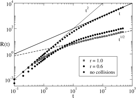
Figure 10: Self-diffusion: behavior of $R(t)$ for three different systems: one without collisions (free particles), one with elastic collisions and the third with inelastic collisions ($r=0.6$).

V.2 Connection between self-diffusion and structure

We follow Alexander and Pincus pincus argument in order to derive a formula for the self-diffusion and show the connection with the compressibility of the system. Let us consider the two time correlator:

$$\langle\rho_{k}(t)\rho_{-k}(0)\rangle=\sum_{ij}\langle e^{ikx_{i}(t)}e^{-ikx_{j}(0)}\rangle$$ (25)

we set $x_{i}(t)=X_{i}+(x_{i}(t)-X_{i})=X_{i}+u_{i}$, where $X_{i}$ are the nodes of the 1D lattice $X_{i}=ia$, ($a$ being the lattice spacing). Expanding around $X_{i}$

$$\langle\rho_{k}(t)\rho_{-k}(0)\rangle\simeq k^{2}\sum_{ij}\mbox{e}^{ik(X_{i}-X_{j})}\langle u_{i}(0)u_{j}(t)\rangle$$ (26)

hence

$$\langle\hat{u}_{k}(t)\hat{u}_{-k}(0)\rangle=\frac{\langle\rho_{k}(t)\rho_{-k}(0)\rangle}{Nk^{2}}$$ (27)

We assume, now, that the density correlator varies as

$$\langle\rho_{k}(t)\rho_{-k}(0)\rangle=\langle\rho_{k}(0)\rho_{-k}(0)\rangle e^{-Dk^{2}t}$$ (28)

where $D=D_{0}/S(0)$ (this is demonstrated in Appendix A) is the collective diffusion coefficient, with $D_{0}=T_{b}/\gamma$. Now, the mean square displacement per particle (21) can be written as $R(t)=\sum_{l}\langle[u_{l}(t)-u_{l}(0)]^{2}\rangle/N$ and, in Fourier components, reads

$$R(t)=\frac{2}{N}\sum_{k}\langle\hat{u}_{k}(0)\hat{u}_{-k}(0)-\hat{u}_{k}(t)\hat{u}_{-k}(0)\rangle$$ (29)

employing Eq. 27 we find

$$R(t)=2\sum_{k}\langle\rho_{k}(0)\rho_{-k}(0)\rangle\frac{1-{\mbox{e}}^{-Dk^{2}t}}{N^{2}k^{2}}$$ (30)

Approximating the sum with an integral ($\sum_{k}\to L/(2\pi)\int_{-\pi/a}^{\pi/a}dk$ and recalling that

$$NS(k)=\langle\rho_{k}(0)\rho_{-k}(0)\rangle$$ (31)

we obtain

$$R(t)=\frac{2L}{N}\int_{0}^{\pi/a}\frac{dk}{2\pi}S(k)\frac{1-\mbox{e}^{-Dk^{2}t}}{k^{2}}$$ (32)

and therefore

$$R(t)\simeq\frac{2}{\rho\pi}S(0)\sqrt{\pi Dt}=\frac{2}{\rho}\sqrt{\frac{D_{0}S(0)t}{\pi}}$$ (33)

Notice that such a formula in the case of hard-rods is identical to formula (24).

We see that the tagged particle diffusion depends on the structure of the fluid. In the granular fluid the $k\to 0$ part of the spectrum is enhanced and thus we expect a stronger tagged particle diffusion. This is what we observe. Physically there are larger voids and particles can move more freely. Let us notice that as far as the collective diffusion is involved the spread of a group of particles is faster in the presence of repulsive interactions than without. tarazona

VI Conclusions

In this paper we have studied a one-dimensional system of inelastic hard-rods coupled to a stochastic heat-bath with the idea that it can represent a reference system in the area of granular gases to test theories and approximations. Due to the relative simplicity of the one dimensional geometry we have shown that it is possible to obtain relations between the macroscopic control parameters such as kinetic temperature, pressure and density. We tested these analytical predictions against the numerical measurements and found a fairly good agreement. It also appears that many properties of the heated one-dimensional inelastic hard rod system are similar to those of ordinary fluids. However, when we have considered how various physical observables fluctuate about their equilibrium values, many relevant differences have emerged. These range from the non-Gaussian behavior of the velocity distribution, the peculiar form of the distribution of distances between particles and of the energy fluctuations to the shape of the structure factor at small wave-vectors. Finally, we have found that the diffusive properties of the system are affected by the inelasticity and in particular the self-diffusion is enhanced.

To conclude, in spite of the similarity between ordinary fluids and granular fluids, which has been recognized for many years and has made possible to formulate hydrodynamical equations for granular media in rapid, dilute flow, the presence of anomalous fluctuations in the inelastic case indicates the necessity of a treatment which incorporates in a proper way both the local effects such as the excluded volume constraint and the long ranged velocity and density correlations. Such a program has been partially carried out by Ernst and coworkers Ernstprogram , but needs to be completed regarding the description of the fluid structure.

VII Appendix A

In the case of over-damped dynamics (i.e. large values of $\gamma$) one finds that the collective diffusion is given by tarazona

$$\frac{\partial\rho(x,t)}{\partial t}=\frac{1}{\gamma}\frac{\partial}{\partial x}\bigg{\{}\rho(x,t)\frac{\partial\mu(\rho(x))}{\partial x}\bigg{\}}$$ (34)

where $\mu(\rho(x))$ is the local chemical potential. Expanding $\mu$ about its average value $\rho_{0}$ we obtain:

$$\frac{\partial\mu(\rho(x))}{\partial x}=\bigg{[}\frac{\delta\mu}{\delta\rho}\bigg{]}_{\rho_{0}}\frac{\partial\rho(x)}{\partial x}$$ (35)

Substituting into Eq. (34) we find

$$\frac{\partial\rho(x,t)}{\partial t}=\frac{1}{\gamma}\rho_{0}\bigg{[}\frac{\delta\mu}{\delta\rho}\bigg{]}_{\rho_{0}}\frac{\partial^{2}\rho(x)}{\partial x^{2}}$$ (36)

and using

$$S(0)=\frac{K_{B}T_{b}}{\rho_{0}}\bigg{[}\frac{\partial\rho_{0}}{\partial\mu}\bigg{]}_{T}$$ (37)

in the case of elastic hard rods we obtain:

$$\frac{\partial\rho(x,t)}{\partial t}=\frac{1}{\gamma}\frac{K_{B}T_{b}}{S(0)}\frac{\partial^{2}\rho(x)}{\partial x^{2}}=\frac{D_{0}}{S(0)}\frac{\partial^{2}\rho(x)}{\partial x^{2}}$$ (38)

Thus the renormalized diffusion coefficient is $D=D_{0}/S(0)$.

References

- (1) H.M. Jaeger, S.R. Nagel and R.P. Behringer, Rev. Mod. Phys. 68, 1259 (1996) and references therein.
- (2) J. Duran, Sands, Powders and Grains: An Introduction to the Physics of Granular Materials (Springer-Verlag, New York, 2000).
- (3) L.P. Kadanoff, Rev. Mod. Phys. 71, 435 (1999).
- (4) Granular Gases, Lectures Notes in Physics vol.564, T. Pöschel and S. Luding editors, Berlin Heidelberg, Springer-Verlag (2001).
- (5) J.P. Hansen and I.R. MacDonald, Theory of Simple Liquids, Academic Press: London, 1990.
- (6) Lord Rayleigh, Nature 45, 80 (1995).
- (7) L. Tonks, Phys. Rev. 50, 955 (1936).
- (8) H. Takahashi, Proc. Phys. Math. Soc. Japan 24, 60 (1942).
- (9) J. Frenkel, Kinetic Theory of Liquids, Oxford University Press, New York, 1940.
- (10) F. Gursey, Proc. Cambridge Philos. Soc. 46, 182 (1950).
- (11) Z. Salsburg, R. Zwanzig and J. Kirkwood, J.Chem.Phys. 21, 1098 (1953).
- (12) J.K. Percus, J.Stat.Phys. 15, 505 (1976).
- (13) J.M. Pasini and P. Cordero, Phys. Rev. E 63, 041302 (2001).
- (14) N. Sela and I. Goldhirsch, Phys. Fluids 7, 507 (1995).
- (15) S. McNamara and W.R. Young, Phys. Fluids A 4, 496 (1992); ibid. 5, 34 (1993).
- (16) E.L. Grossman and B. Roman, Phys. Fluids 8, 3218 (1996).
- (17) T. Zhou, Phys. Rev. Lett 80, 3755 (1998).
- (18) T. Zhou, Phys. Rev. E 58, 7587 (1998).
- (19) Y. Du, H. Li, and L. P. Kadanoff, Phys. Rev. Lett. 74 1268 (1995).
- (20) D.R.M. Williams and F.C. MacKintosh, Phys. Rev. E 54, R9 (1996).
- (21) A. Puglisi, V. Loreto, U.M.B. Marconi, A. Petri, and A. Vulpiani, Phys. Rev. Lett. 81, 3848 (1998) and Phys. Rev. E 59, 5582 (1999).
- (22) F. Cecconi, A. Puglisi, U.M.B. Marconi and A. Vulpiani, Phys. Rev. Lett. 59, 064301 (2003).
- (23) E. Ben-Naim, S.Y. Chent, G.D. Doolent, and S. Redner, Phys. Rev. Lett. 83 4069 (1999).
- (24) A. Baldassarri, U. Marini Bettolo Marconi and A. Puglisi, Europhys. Lett. 58, 14 (2002).
- (25) M.P. Allen and D.J.Tildesley, Computer Simulation of Liquids, Clarendon Press, Oxford, (1987).
- (26) A. Barrat and E. Trizac, Phys. Rev. E 66, 051303 (2002).
- (27) J.J. Erpenbeck and W.W. Wood, Statistical Mechanics B. Modern Theoretical Chemistry, ed. J. Berne, vol. 6, Plenum, New York, (1977).
- (28) W. Losert, D.G.W. Cooper, J. Delour, A. Kudrolli and J.P. Gollub, Chaos, 9, 682 (1999).
- (29) K. Feitosa and N. Menon, Phys. Rev. Lett. 88, 198301 (2002).
- (30) Daniel L. Blair and A. Kudrolli, Phys. Rev. E 67, 041301 (2003).
- (31) J.S. Olafsen and J.S. Urbach, Phys. Rev. Lett. 81 , 4369 (1998).
- (32) I.S. Aranson and J.S. Olafsen, Phys. Rev. E 66, 061302 (2002).
- (33) A. Kudrolli and J. Henry, Phys. Rev. E 62, R1489 (2000).
- (34) J.J. Brey and M.J. Ruiz-Montero Phys. Rev. E 67, 021307 (2003).
- (35) T.P.C. van Noije and M.H. Ernst, Granular Matter 1, 57 (1998).
- (36) K. Huang, Statistical mechanics, J. Wiley & Sons, New York, 1987.
- (37) T.P.C. van Noije, M.H. Ernst, E. Trizac, and I. Pagonabarraga, Phys. Rev. E 59, 4326 (1999).
- (38) I. Goldhirsch and G. Zanetti, Phys. Rev. Lett. 70 1619 (1993).
- (39) D. Paolotti, C. Cattuto, U. Marini Bettolo Marconi, and A. Puglisi, Granular Matter 5, 75 (2003).
- (40) T.P.C. van Noije, M.H. Ernst, R. Brito, and J.A.G. Orza, Phys. Rev. Lett. 79 (1997).
- (41) M. Kollmann, Phys. Rev. Lett. 90, 180602 (2003).
- (42) J.L. Lebowitz and J.K. Percus, Phys. Rev. 155, 122 (1967).
- (43) T.E. Harris, J. Appl. Prob. 2, 323 (1965).
- (44) S. Alexander and P. Pincus, Phys. Rev. B 18, 2011 (1978).
- (45) H. van Beijeren, K.W. Kehr and R. Kutner, Phys. Rev. B 28, 5711 (1983).
- (46) U. Marini Bettolo Marconi and P. Tarazona J. Chem. Phys.110, 8032 (1999) and J. Phys: Condens. Matter 12 A413 (2000).