Exact scaling functions of the multichannel Kondo model

Abstract

We reinvestigate the large degeneracy solution of the multichannel Kondo problem, and show how in the universal regime the complicated integral equations simplifying the problem can be mapped onto a first order differential equation. This leads to an explicit expression for the full zero-temperature scaling functions at - and away from - the intermediate Non Fermi Liquid fixed point, providing complete analytic information on the universal low - and intermediate - energy properties of the model. These results also apply to the widely-used Non Crossing Approximation of the Anderson model, taken in the Kondo regime. An extension of this formalism for studying finite temperature effects is also proposed and offers a simple approach to solve models of strongly correlated electrons with relevance to the physics of heavy fermion compounds.

Models of quantum impurities constitute a central piece in our understanding of strongly correlated systems, as demonstrated by the importance of these ideas for the physical description of magnetic impurities in metals Hewson (1996) or superconductors Pan et al. (2000); Polkovnikov et al. (2001), the correlation-driven metal to insulator transition Georges et al. (1996), the behavior of heavy fermion compounds Lee et al. (1986); Schröder et al. (2000), and the coherent transport through nanostructures Kouwenhoven and Glazman (2001). Despite of their relative simplicity, one usually has recourse to different techniques in order to fully grasp the complete physics displayed by these localized hamiltonians. Unfortunately, analytical approximation schemes devised to deal with the Kondo problem, like the slave boson method Newns and Read (1987), lead in general to too much simplifications. On the contrary, purely numerical methods Krishna-murthy et al. (1980) or exact techniques Andrei and Destri (1984) provide quantitative results, but often lack the flexibility to solve more interesting cases, like lattice impurity models, or to compute dynamical observables. Conformal field theory (CFT) can also provide interesting insights on this problem Affleck and Ludwig (1993), which is however limited to the elucidation of the critical behavior right at the possible fixed points.

Another way of tackling impurity hamiltonians lies in setting up controlled limits that lead to a simplified solution encompassing all physical aspects of the problem. We will focus here on a large number of channels limit of quantum impurity models that was proposed previously Parcollet et al. (1998); Parcollet and Georges (1997), from which the well-studied Cox and Ruckenstein (1993); Bickers (1987) self-consistent pertubation theory (Non Crossing Approximation or NCA) appears to be a limiting case. However simplified, this alternative approach is known to lead to challenging non-linear integral equations, from which limited analytical information can be gathered Parcollet et al. (1998); Mueller-Hartmann (1984). A numerical solution of these equations is often possible, but is increasingly difficult to obtain at low temperature and for real frequency quantities. Thus little work has been undertaken using this method for the many interesting extensions of the Kondo model, like multi-impurity hamiltonians or the Kondo lattice. This is unfortunate, as this technique offers a concrete opportunity for building a consistent theory for the competition of Kondo screening and magnetism Parcollet and Georges (1997) which lies at the heart of the quantum criticality displayed in heavy fermions compounds.

We will show in this paper that much progress can be made towards both analytic and numerical solutions of the multichannel Kondo model. Indeed we are able for the first time to solve this problem at zero temperature in the universal regime (when the Fermi energy is large compared to frequency). The key step of this solution lies in the mapping of the saddle-point integral equations onto a much simpler non-linear differential equation, that can be solved explicitely. Our calculation follows the well-known analysis by Mueller-Hartmann of the similar NCA equations for the infinite $U$ Anderson impurity model Mueller-Hartmann (1984). However the Kondo regime of these equations seems not to have been considered previously in the literature, and constitutes the originality of the present work with respect to Mueller-Hartmann (1984). We are thus able to obtain analytic expressions for the frequency-dependent scaling functions, for the Kondo temperature and for the precise location of the intermediate Non Fermi Liquid fixed point. This offers also new insights on quantum criticality: we introduce below a concept of complex Kondo temperature and describe an interesting crossover phase diagram around the intermediate coupling fixed point. We will finally show how these ideas can be formulated at finite temperature, by deriving non-linear finite difference equations for the Green’s functions, that may be useful to solve numerically more challenging extensions of the present problem.

Considering the Kondo model from now on, we will be interested here in a multichannel version that consists of a SU($N$) spin antiferromagnetically coupled to $K$ channels of conduction electrons, as expressed by the hamiltonian:

$$H=\sum_{k,\sigma,\alpha}\epsilon_{k}c^{\dagger}_{k\sigma\alpha}c_{k\sigma\alpha}+\frac{J_{K}}{N}\sum_{kk^{\prime}\sigma\sigma^{\prime}\alpha}S_{\sigma^{\prime}\sigma}c^{\dagger}_{k\sigma\alpha}c_{k^{\prime}\sigma^{\prime}\alpha}$$ (1)

using a fermionic representation $S_{\sigma^{\prime}\sigma}=f^{\dagger}_{\sigma^{\prime}}f_{\sigma}-q_{0}\delta_{\sigma\sigma^{\prime}}$ of the localized spin, where $\sigma=1\ldots N$. The constraint $\sum_{\sigma}f_{\sigma}^{\dagger}f_{\sigma}=q_{0}N$ should also be enforced. Here the parameter $q_{0}N$ may be understood as the size of the quantum spin, and the channel index $\alpha$ is taken to run from $1$ to $K$.

In a previous work Parcollet et al. (1998), Parcollet and Georges have shown how this model could be simplified in the limit where both $N$ and $K$ are large, keeping $\gamma=K/N$ fixed (the fact that the spin size $q_{0}N$ is taken to be large is also an important point in obtaining their solution). Introducing the spinon propagator $G_{f}(\tau)=-\big{<}T_{\tau}f_{\sigma}(\tau)f_{\sigma}^{\dagger}(0)\big{>}$ and the Green’s function $G_{B}(\tau)=+\big{<}T_{\tau}B_{\alpha}(\tau)B^{\dagger}_{\alpha}(0)\big{>}$ of the channel bosonic field $B_{\alpha}(\tau)$ conjugate to the operator $\sum_{k\sigma}c^{\dagger}_{k\sigma\alpha}f_{\sigma}$, the saddle-point equations read (in imaginary time):

$$\Sigma_{f}(\tau) = \gamma G_{0}(\tau)G_{B}(\tau)$$ (2)

$$\Sigma_{B}(\tau) = -G_{0}(-\tau)G_{f}(\tau)=G_{0}(\tau)G_{f}(\tau)$$ (3)

for a particle-hole symmetric bath Green’s function $G_{0}(i\omega)\equiv\sum_{k}1/(i\omega-\epsilon_{k})$. The self-energies in the previous set of equations are given by the Dyson equations:

$$G_{f}^{-1}(i\omega_{n}) = i\omega_{n}+\lambda-\Sigma_{f}(i\omega_{n})$$ (4)

$$G_{B}^{-1}(i\nu_{n}) = \frac{1}{J_{K}}-\Sigma_{B}(i\nu_{n})$$ (5)

where $\omega_{n}$ ($\nu_{n}$) denotes a fermionic (bosonic) Matsubara frequency. The Lagrange multiplier $\lambda$ is used to enforce the constraint related to the spin size, which reads in the large $N$ limit:

$$G_{f}(\tau=0^{-})=q_{0}$$ (6)

The usual NCA equations Cox and Ruckenstein (1993) are obtained when the constraint $\sum_{\sigma}f_{\sigma}^{\dagger}f_{\sigma}=1$ is performed exactly, and this amounts to take the $q_{0}\rightarrow 0$ limit in the saddle-point equations. It is useful to analytically continue equations (2)-(3), and one readily obtains in terms of retarded quantities at zero temperature Florens and Georges (2002):

$$\Sigma_{f}(\omega) = \gamma\int_{0}^{+\infty}\frac{{{\mathrm{d}}}\epsilon}{\pi}G_{0}^{\prime\prime}(\epsilon)\big{[}G_{B}(\omega\!-\!\epsilon)-J_{K}\big{]}$$ (7)

$$-\gamma\int_{\omega}^{+\infty}\frac{{{\mathrm{d}}}\epsilon}{\pi}G_{0}(\epsilon)G_{B}^{\prime\prime}(\omega\!-\!\epsilon)$$

$$\Sigma_{B}(\omega) = \int_{0}^{+\infty}\frac{{{\mathrm{d}}}\epsilon}{\pi}G_{0}^{\prime\prime}(\epsilon)G_{f}(\omega-\epsilon)$$ (8)

$$-\int_{\omega}^{+\infty}\frac{{{\mathrm{d}}}\epsilon}{\pi}G_{0}(\epsilon)G_{f}^{\prime\prime}(\omega-\epsilon)$$

where double primed quantities denote imaginary parts. The subtracted $J_{K}$ in (7) comes from a careful inspection of the short time behavior of $G_{B}(\tau)$. As we are interested in the universal regime where the Fermi energy of the conduction electrons is the biggest energy scale, we follow Mueller-Hartmann (1984) and consider a flat density of states of half-width $\Lambda$: $G_{0}(\omega)\simeq iG_{0}^{\prime\prime}(\omega)=-i\pi\rho_{0}\theta(\Lambda^{2}-\epsilon^{2})$, with $\rho_{0}=1/(2\Lambda)$ (the real part of $G_{0}$ can be discarded to order $\Lambda^{-1}$). This leads in the previous equations to integrals running from the lower bound $\epsilon_{{\mathrm{min}}}=\omega-\Lambda$ that can be replaced by $\epsilon_{{\mathrm{min}}}\simeq-\Lambda$ for frequency smaller than $\Lambda$. This trick allows to obtain simple expressions for the self-energies:

$$\Sigma_{f}(\omega)\! = \!-\gamma\rho_{0}\int_{-\Lambda}^{\omega}\!\!\!{{\mathrm{d}}}\epsilon\big{[}G_{B}(\epsilon)-J_{K}\big{]}+i\gamma\rho_{0}\int_{-\Lambda}^{0}\!\!\!{{\mathrm{d}}}\epsilon\;G_{B}^{\prime\prime}(\epsilon)$$

$$\Sigma_{B}(\omega)\! = \!-\rho_{0}\int_{-\Lambda}^{\omega}\!\!\!{{\mathrm{d}}}\epsilon\;G_{f}(\epsilon)+i\rho_{0}\int_{-\Lambda}^{0}\!\!\!{{\mathrm{d}}}\epsilon\;G_{f}^{\prime\prime}(\epsilon)$$ (9)

that lead by differentiation to the following relations:

$$\frac{\partial}{\partial\omega}\Sigma_{f}(\omega) = -\gamma\rho_{0}\big{[}G_{B}(\omega)-J_{K}\big{]}$$ (10)

$$\frac{\partial}{\partial\omega}\Sigma_{B}(\omega) = -\rho_{0}G_{f}(\omega)$$ (11)

Equation (9) imply also the following boundary condition at the lower band edge (for $\Sigma_{B}$):

$$\Sigma_{B}(-\Lambda)=i\rho_{0}\int_{-\Lambda}^{0}\!\!\!{{\mathrm{d}}}\epsilon\;G_{f}^{\prime\prime}(\epsilon)$$ (12)

Following Mueller-Hartmann (1984), we now define the inverse propagators $Y_{f}(\omega)\equiv-G_{f}^{-1}(\omega)$ and $Y_{B}(\omega)\equiv G_{B}^{-1}(\omega)$. Combining the previous two relations with the Dyson equations (4)-(5) for real frequencies, we easily arrive to:

$$\frac{1}{Y_{f}}\frac{\partial}{\partial\omega}Y_{f} = \frac{1-\gamma\rho_{0}J_{K}}{\rho_{0}}\frac{\partial}{\partial\omega}Y_{B}+\gamma\frac{1}{Y_{B}}\frac{\partial}{\partial\omega}Y_{B}$$ (13)

$$Y_{f}^{-1} = -\frac{1}{\rho_{0}}\frac{\partial}{\partial\omega}Y_{B}$$ (14)

The first equation provides a first constant of motion, that reads:

$$\log\big{[}-Y_{f}(\omega)\big{]}+C=\frac{1-\gamma\rho_{0}J_{K}}{\rho_{0}}Y_{B}(\omega)+\gamma\log Y_{B}(\omega)$$ (15)

where $C$ is determined by the boundary condition (12). The crucial difference between the multichannel Kondo model we consider in this paper and previous work Mueller-Hartmann (1984) on the NCA for the infinite $U$ Anderson model is that, by inserting relation (14) into (15), we obtain a first order differential equation:

$$\frac{\partial}{\partial\omega}Y_{B}=\rho_{0}e^{C}(Y_{B})^{-\gamma}e^{(1-\gamma\rho_{0}J_{K})Y_{B}/\rho_{0}}$$ (16)

instead of a non-linear second order differential equation. Ultimately, this simplification is due to the disappearance of the high-energy scale associated with charge fluctuations on the impurity. We emphasize however that this result also applies to the usual NCA of the Anderson model, in the Kondo regime.

To exhibit the exact solution of the multichannel Kondo model, we introduce two functions $f^{\pm}_{\gamma}(x)$ defined by the integral (which is easily computed for integer $\gamma$):

$$x=\int_{0}^{f^{\pm}_{\gamma}(x)}{{\mathrm{d}}}t\;e^{\pm t}\;t^{\gamma}$$ (17)

and thus obtain the following scaling form of the inverse bosonic propagator:

$$Y_{B}(\omega) = Af^{a}_{\gamma}(\omega/z_{K})$$ (18)

$${{\mathrm{where}}}\;\;\;a = {{\mathrm{Sign}}}(1-\gamma\rho_{0}J_{K})$$ (19)

The numerical prefactor in the previous equation is given by $A\equiv\rho_{0}/|1-\gamma\rho_{0}J_{K}|$, and a complex Kondo temperature $z_{K}\equiv\rho_{0}^{\gamma}|1-\gamma\rho_{0}J_{K}|^{-1-\gamma}e^{C}$ has to be introduced. The fact that the propagators scale with respect to a complex energy scale stems from the presence of a spectral asymmetry for generic values of $q_{0}$ Parcollet et al. (1998).

Equation (18) can be considered to be the complete solution of the large number of channels Kondo model for all energy scales below the high energy cut-off, and constitutes the central result of our paper. In particular, it is valid for frequency below and above the the Kondo temperature, defined as $T_{K}\equiv|z_{K}|$, as long as $T_{K}$ is much smaller than the cut-off $\Lambda$. To analyze the properties of this scaling function is first particularly simple right at the Non Fermi Liquid fixed point. Indeed, equation (16) allows to locate the coupling $J_{K}^{*}=1/(\rho_{0}\gamma)$ at which the various propagators exihibit scale invariance:

$$Y_{B}(\omega)=\big{[}\rho_{0}(1+\gamma)e^{C}\omega\big{]}^{1/(1+\gamma)}\;\;{{\mathrm{at}}}\;\;J_{K}=J_{K}^{*}$$ (20)

for all frequencies smaller than the cut-off. We note also that, away from the fixed point $J_{K}^{*}$, the behavior (20) still applies, albeit for $\omega<T_{K}$. The power law obtained in equation (20) agrees with previous work Mueller-Hartmann (1984); Parcollet et al. (1998), in which the zero-temperature low-frequency propagator $G_{B}(\omega)\propto\omega^{2\Delta_{B}-1}$, with $2\Delta_{B}=\gamma/(1+\gamma)$, was obtained. For frequencies comparable to $T_{K}$ and away from the fixed point, equation (18) leads to universal corrections to this pure power law behavior, a result that could not be obtained from the low frequency analysis performed in Parcollet et al. (1998). The various regimes observed are expressed graphically in figure 1.

Figure 1: Zero temperature $(\omega,J_{K})$ crossover diagram: the dashed line represents the Kondo temperature $T_{K}$ below which Non Fermi Liquid (NFL) behavior is observed; above this line two universal crossover regimes described in the text are characterized by the scaling functions (18). For $|\omega|\gtrsim\Lambda$, non universal corrections start to appear.

To understand first the universal crossover arising at $J_{K}<J_{K}^{*}$, we consider large frequency above $T_{K}$, and get $Y_{B}(\omega)\propto\log|\omega|$, so that $G_{f}(\omega)\propto 1/\omega$ from equation (14). This corresponds to a free moment regime, where the impurity spin is weakly bound to the screening cloud of the conduction electrons. The scaling function $f_{\gamma}^{+}(x)$ thus describes the crossover from weak coupling to the fixed point $J_{K}^{*}$ Nozières and Blandin (1980). From the same token, $f_{\gamma}^{-}(x)$ is associated to the flow from strong to intermediate coupling; we note however that in the case $J_{K}>J_{K}^{*}$ one has roughly $T_{K}\sim\Lambda/\Gamma(\gamma+1)$, so that the condition $T_{K}\ll\Lambda$ (and hence universality of this regime) is met only for $\gamma\gg 1$. This picture of the various crossover regimes that we have obtained is particularly explicit, and illustrates the renormalization flow around the attractive fixed point. To make contact with the theory of quantum critical phenomena Sachdev (2000), we emphasize that $J_{K}$ is for the multichannel Kondo model an irrelevant perturbation around $J_{K}^{*}$, so that no phase transition occurs as $J_{K}$ is varied. Therefore the low energy behavior at all $J_{K}$ is controlled by the intermediate fixed point, in contrast to the case of a relevant tuning parameter driving a true quantum phase transition.

Another way to depict the crossovers taking place around $J_{K}^{*}$ is to plot the scaling functions $f_{\gamma}^{\pm}(x)$, figure 2.

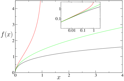
Figure 2: Plot on both linear and logarithmic scales of the scaling functions $f^{+}_{\gamma}(x)$ (lower curve) and $f^{-}_{\gamma}(x)$ (upper curve) for $\gamma=1$, as compared to their low energy asymptotic form $[(1+\gamma)x]^{1/(1+\gamma)}$ (middle curve).

It is also possible to compute the exact value for the Kondo temperature $T_{K}$. We will do this in the limit $q_{0}\rightarrow 0$, which corresponds actually to the usual Non Crossing Approximation. In this case, the pseudo-particle propagators get maximally asymmetric, and the spectral functions $G_{B}^{\prime\prime}(\omega)$ and $G_{f}^{\prime\prime}(\omega)$ vanish for all $\omega<0$. This implies an explicit expression for the boundary condition (12), $\Sigma_{B}(-\Lambda)=0$, and a purely real inverse propagator $Y_{B}(\omega)$ (for negative frequency). The initial condition $Y_{B}(-\Lambda)=1/J_{K}$ gives for $J_{K}<J_{K}^{*}$ the following relation:

$$\frac{T_{K}}{\Lambda}=\left[\int_{0}^{1/(\rho_{0}J_{K})-\gamma}\;{{\mathrm{d}}}t\;e^{t}\;t^{\gamma}\right]^{-1}$$ (21)

In the limit of small $J_{K}$, one finds:

$$T_{K}\simeq\Lambda(\rho_{0}J_{K})^{\gamma}e^{\gamma}e^{-1/(\rho_{0}J_{K})}$$ (22)

i.e. a vanishingly small Kondo temperature, as expected. When $J_{K}$ approaches the fixed point value $J_{K}^{*}$, $T_{K}$ is maximum and Non Fermi Liquid properties apply up to the high energy cutoff.

We now discuss temperature effects. In Parcollet et al. (1998) was shown how to obtain from the large-$N$ equations (2-5) the exact finite-temperature low-frequency (i.e. $\omega\ll T_{K}$) scaling functions using CFT arguments. It seems unfortunately impossible to apply this approach to extend our exact scaling function (18), valid for $T_{K}\sim\omega\ll\Lambda$, to finite temperature. However we can succeed in generalizing the derivation of the linear differential equations (10-11) to the case of non zero temperature. For that purpose we consider the imaginary time saddle-point equations in the scaling regime:

$$\Sigma_{f}(i\omega_{n}) = -\gamma\int_{0}^{\beta}\!\!\!\!d\tau e^{i\omega_{n}\tau}\frac{\pi\rho_{0}}{\beta\sin(\pi\tau/\beta)}\big{[}G_{B}(\tau)-J_{K}\big{]}$$

$$\Sigma_{B}(i\nu_{n}) = -\int_{0}^{\beta}\!\!\!\!d\tau e^{i\nu_{n}\tau}\frac{\pi\rho_{0}}{\beta\sin(\pi\tau/\beta)}G_{f}(\tau)$$ (23)

This gives the idea of writing a finite difference equation for the self-energies, which provides indeed a remarkably simple result:

$$\!\!\!\!\!\frac{\Sigma_{f}(i\nu_{n}+i\pi/\beta)-\Sigma_{f}(i\nu_{n}-i\pi/\beta)}{2\pi/\beta}\!\!\! = \!\!\!-i\gamma\rho_{0}\big{[}G_{B}(i\nu_{n})-J_{K}\big{]}$$

$$\!\!\!\!\!\frac{\Sigma_{B}(i\omega_{n}+i\pi/\beta)-\Sigma_{B}(i\omega_{n}-i\pi/\beta)}{2\pi/\beta}\!\!\! = \!\!\!-i\rho_{0}G_{f}(i\omega_{n})$$ (24)

Although these relations do not lead to much analytical understanding as compared to their zero temperature counterpart, they offer an economical way of tackling the finite temperature integral equations, which may be of interest for some generalizations of the Kondo model.

We would like to conclude the paper on the possible applications of the formalism discussed in this work. Our main result, the computation of the full zero-temperature scaling functions of the many channel Kondo model, offers perspectives both in the physics of quantum impurities and strongly correlated systems. First, questions that we will address in future work concern the direct comparison of the exact scaling function (18) to the numerical solution of the large-N integral equations (2-5), using both the standard numerical routines with fast Fourier fransforms and the system of finite difference equations (24). In the same direction, it would also be interesting to perform a similar analysis and gain some analytical insight on the multichannel Kondo model in the bosonic representations Parcollet and Georges (1997), a model that allows a richer phase diagram with a transition from over-screening to underscreening.

As was pointed out in the introduction, models of several quantum impurities or lattice versions of the Kondo hamiltonian are of great experimental importance and notoriously difficult to tackle theoretically. We hope that the analytical step undertaken in the present work will allow further progress in this direction.