One dimensional gapless magnons in a single anisotropic ferromagnetic nanolayer

Abstract

Gapless magnons in a plane ferromagnet with normal axis anisotropy are shown to exist besides the usual gapped modes that affect spin dependent transport properties only above a finite temperature. These magnons are one dimensional objects, in the sense that they are localized inside the domain walls that form in the film. They may play an essential role in the spin dependent scattering processes even down to very low temperatures.

While charge and its transport play an essential role in carrying and processing information, spin is the origin of magnetism and is the basis to most of the storage devices in information-related technologies. There is much interest in combining charge and spin properties in order to expand the possibilities for applications into the so called spintronics wolf . This field, that has started with the discovery of giant magnetoresistance (GMR) in alternating Fe/Cr layers baib , has rapidly become on focus with the report of magnetic materials with high transition temperatures ($T_{C}$) such as Ga_1-xMn_xAs ($T_{C}\sim 110$ K) ohno and Ti_1-xCo_xO₂ ($T_{C}\sim 300$ K) ticoo , for instance. With the upscaling of $T_{C}$ toward room temperatures realizations of practical ideas ensue, pointing in the direction of spin-based devices analogous to $p$-$n$ transistors vig . Functioning principles of such devices rely on the existence of domain walls (DW) in finite ferromagnetic samples. The role of DW on transport of electrical current has been shown in the early experiments on iron whyskerstaylor and since then subjected to intense experimental and theoretical investigation various . The possibility that GMR originates directly from DW may yield the fabrication of GMR devices from single layered materials taking simultaneous advantage of spin and charge degrees of freedom. With the improvement of growing techniques, the possibilities of producing 2D ferromagnetic samples with DW of few tenths of Å, has become reality sample .

In this Letter we report on a magnetic excitation that has not yet been accounted for the scattering of electrons by DW. One-dimensional (1D) gapless magnons propagating inside a DW of a single-layer ferromagnet are shown to exist in addition to the usually known gapped magnons. Starting from an appropriate model hamiltonian, we solve it for the continuum limit in 2D and find that these modes are confined in the 1D DW, as illustrated in Fig.1. Due to the absence of gap, the inelastic coupling of these modes to electrons should manifest at very low temperatures, as opposed to the usual magnon scattering processes that become important only at temperatures comparable to the anisotropy gap. We provide a theory to include the effect of the gapless magnons on conduction electrons.

Figure 1: Domain wall in 2D showing the 1D channel at its center where gapless magnons are expected to propagate in the $y$ direction; the amplitude of such a mode is depicted by the bell-like curve shown on top.

We then present results for the resistivity in a 2D system as a function of the DW size, the electronic density, and the temperature for realistic values of the parameters.

In order to model a system of independent electrons interacting with local $1/2$ spins, we will use the effective hamiltonian ${\cal H}={\cal K}+{\cal H}_{H}+{\cal H}_{I}$, where ${\cal K}$ stands for the electron’s kinetic energy operator $-\hbar^{2}\nabla^{2}/2m$, while ${\cal H}_{H}$ accounts for the interaction between local spins (${\mathbf{S}}_{i}$), described by a 2D ferromagnetic Heisenberg spin hamiltonian

$${\cal H}_{H}=-J\sum_{i}{\mathbf{S}}_{i}\cdot{\mathbf{S}}_{i+1}-J\Delta\sum_{i}({\rm S}_{i}^{z})^{2},$$ (1)

on a square lattice of constant $a$. Here $\Delta>0$ gives the strength of the on-site anisotropy and $J>0$ is the exchange amplitude. Interaction between electrons and the local spins is considered through

$${\cal H}_{I}=-J_{K}a^{2}\sum_{i}{\bm{\sigma}}\cdot{\mathbf{S}}_{i}\delta({\mathbf{r}}_{i}-{\mathbf{r}})$$ (2)

where $J_{K}$ is the exchange integral and ${\bm{\sigma}}$ is the spin of the electron.

First, we consider the static DW solution of ${\cal H}_{H}$ for a $\pi$-domain. In the continuum the following hydrodynamic equations are obtained for the magnetization,

$$\frac{\partial\theta}{\partial t}=-j(\sin\theta\nabla^{2}\phi+2\cos\theta\nabla\theta\cdot\nabla\phi),$$ (3)

and

$$\frac{\partial\phi}{\partial t}=j\left(\frac{\nabla^{2}\theta}{\sin\theta}-\cos\theta(\nabla\phi)^{2}-\frac{1}{\lambda^{2}}\cos\theta\right),$$ (4)

with $j\equiv JS^{2}a^{2}/\hbar$ and $\lambda\equiv a/\sqrt{2\Delta}$. The fields $\theta$ and $\phi$ parametrize the magnetization through the usual relation ${\bm{S}}({\mathbf{r}})=S(\sin{\theta}\cos{\phi},\sin{\theta}\sin{\phi},\cos{\theta})$. Such a hydrodynamic treatment suits the low energy excitations studied in what follows, hence the continuum limit is not only appropriate but becomes exact for the long wavelength phenomena handled below.

It is possible to find a static solution for these coupled equations in the form of a $\pi$ DW. Assuming $\phi=\bar{\phi}$ is constant, $\theta=\bar{\theta}(x)$ (see Fig.1), and using the boundary conditions $\lim_{x\rightarrow\mp\infty}\cos\theta(x)=\pm 1$, the coupled equations can be easily integrated to give $\bar{\bm{S}}({\mathbf{r}})=S[\hat{\bm{x}}\;{\rm sech}(x/\lambda)-\hat{\bm{z}}\tanh(x/\lambda)]$ if we conveniently choose $\bar{\phi}=0$.

Hence a $\pi$ DW like the one illustrated in Fig.1 is admitted as an equilibrium configuration in the 2D ferromagnetic system described by ${\cal H}_{H}$. One sees that $\lambda$ measures the size of the spin-inversion region thus giving the size of the DW. From the definition of $\lambda$ it is clear that the DW extends throughout the sample unless the anisotropy is different from zero. Strictly, the DW configuration is not the absolute minimum of energy in our model, although it is a stable solution. If one however takes the effect of dipolar interactions, as in a finite sample, the ground state becomes, in general, a DW distortion. Yet, if the temperature is lowered, and as long as the on-site anisotropy $\Delta>0$, one expects to cross a transition temperature below which there are no DW structures in the system. However, in 2D one is able to induce DW’s in a magnetic layer up to a few thousand in a typical sample, even for temperatures as low as a few Ksample . The use of this particular solution as a starting point is then justified, even at the low temperatures for which the excitations studied ahead are more important.

The DW solution for ${\cal H}_{H}$ as obtained here bares resemblance to the solitons studied in the 1D Heisenberg chain wri . As we see below, this similarity with the 1D chain for the equilibrium solution does not lead to the same physics in 2D, the fluctuations about this solution are given by the usual massive magnons plus the additional gapless modes, only present in dimensions $>1$.

We consider small deviations from equilibrium given by $\theta=\bar{\theta}(x)+\xi({\mathbf{r}},t)$ and $\phi=\bar{\phi}+\eta({\mathbf{r}},t)/\sin\bar{\theta}(x)$, where $\xi,\eta\ll 1$. Substitution of these relations in Eqs.(3) and (4) yields $\partial^{2}\xi({\mathbf{r}},t)/\partial t^{2}=-j^{2}[\nabla^{2}-V(x)]^{2}\xi({\mathbf{r}},t)$, where $V(x)\equiv\left(1/\lambda^{2}\right)\left[2\tanh^{2}{\left(x/\lambda\right)}-1\right]$, and an identical equation for $\eta({\mathbf{r}},t)$. Dispersion relations can then be obtained from a standard choice of the solution in the form $\xi({\mathbf{r}},t)=b({\mathbf{r}})\exp{-i\omega}t$, which leads to the following eigenvalue equation,

$$\left[\nabla^{2}-V(x)\right]b({\mathbf{r}})=-\frac{\omega}{j}b({\mathbf{r}}).$$ (5)

It is convenient to study the spectrum of the $x$ dependent solutions to understand why there must be a gap in 1D but not in 2D. This is understood if we realize that Eq.(5) yields the usual discrete eigenvalues associated with the $x$ direction and a mode that is given by just setting $\omega=0$. Let us call this zero eigenvalue solution by zero-mode for further reference. In 1D, the zero-mode is a small static distortion from the original DW solution localized near $x=0$ and with the functional form $\xi(x)\sim{\rm sech}(x/\lambda)$, as it is seen by replacing $x\rightarrow{\mathbf{r}}$ in Eq.(5) and integrating it for $\omega=0$. Since such a mode has no dynamics, the spectrum of the ferromagnetic 1D anisotropic chain is gapped as it is well known. In particular, away from the DW $\lambda^{2}V(x)\rightarrow 1$, and a solution is promptly obtained both in 1D and 2D, in the form of isotropic magnons with a massive spectrum given by $\omega(k)=j(k^{2}+1/\lambda^{2})$ where $k$ is the wave vector. This dispersion holds also in 2D with $k^{2}=k_{x}^{2}+k_{y}^{2}$.

The key ingredient to distinguish 2D from 1D is that with the additional degree of freedom, the zero-mode acquires dynamics and becomes the gapless magnon that we are studying. We see this by using a solution in the form $b({\mathbf{r}})=f(x)g(y)$ in Eq.(5), which separates in

$$\left[\frac{d^{2}}{dx^{2}}-V(x)\right]f(x)=\left(q^{2}-\frac{\omega}{j}\right)f(x),$$ (6)

and

$$g^{\prime\prime}(y)=-q^{2}g(y).$$ (7)

It is clear from these equations that the zero-mode associated with the $x$ direction in Eq.(6) is a propagating spin wave with dispersion given by $\omega(q)=jq^{2}$. In 2D this mode has a finite frequency and is localized about $x=0$, as is seen from the solution $b({\mathbf{r}})\equiv{\rm sech}(x/\lambda)\exp{iqy}$ obtained from integrating Eq.(6) for $\omega(q)=jq^{2}$. An identical solution holds for $\eta({\mathbf{r}},t)$. One can see that $\xi$ is related to transverse ($\perp\hat{\bm{y}}$), while $\eta$ to longitudinal oscillations. The complete solution is given by ${\bm{S}}({\mathbf{r}},t)=\bar{\bm{S}}({\mathbf{r}})+(\partial\bar{\bm{S}}({\mathbf{r}})/\partial\bar{\theta})\xi({\mathbf{r}},t)+\hat{\bm{y}}S\;\eta({\mathbf{r}},t)$, where $\xi$ and $\eta$ are more generally linear combinations of the $q$ and $\omega$ dependent solutions worked out above. The gapless dispersion corresponds to plane magnetization waves propagating with very small amplitudes inside the 1D DW.

It should be pointed that these are not the first gapless excitations reported in a 2D anisotropic chain. Gapless kinks that could propagate under very restricted conditions have been reported previously japas , and they consist basically of topological excitations inside the DW. Within our approximations, Eq.(7) is linear and dispersive and therefore will not sustain such localized kink-like solutions which will ultimately decay into ordinary spin waves. Gapless dispersions have also naturally appeared in solutions of the XXZ hamiltonian in 3D,jafez showing that this is not a particularity of the 2D case we are treating. Here it becomes clear the necessity of dimensions $>1$ for the existence of such wall magnons.

Consideration of these modes for the transport of electrons in magnetic materials appears to be absent from the up to date literature, where magnons are overwhelmingly considered in the analysis of measured data only at temperatures suffciciently high to be comparable to the anisotropy gap, whose typical values range from 50xK to 150xK, depending on the material used. Absence of gap in the spectrum should make the contribution of these objects relevant for the resistivity at lower temperatures.

In what follows, it will be seen that a transport theory for electrons interacting with the gapless magnons can in fact be put forward without complications and that the effects on the resistivity are expected to be quite observable for temperatures much lower than the anisotropy gap.

Hydrodynamics is quantized by writing

$$\widehat{\xi}[qy]=\frac{a}{2\sqrt{L_{y}\lambda}}{\rm sech}\left(\frac{x}{\lambda}\right)\sum_{q}\left[\exp{(iqy)}a_{q}+h.c.\right],$$

and $\widehat{\eta}=\widehat{\xi}[qy-\pi/2]$. This ensures that the contribution of the free magnons in Eq.(1) is written as ${\cal H}_{m}=\sum_{q}\hbar\omega_{q}a^{{\dagger}}_{q}a_{q}$, where $a^{{\dagger}}_{q}$ is the (Heisenberg) bosonic operator that creates a magnon with wave vector $q$, $\hbar\omega_{q}=JS^{2}a^{2}q^{2}$, and $L_{y}$ is the width of the sample.

The electron-magnon interaction given by Eq.(2), can be put in the form ${\cal H}_{I}=U_{0}(x)+U_{1}(x)+{\cal H}_{em}$, where $U_{0}(x)=SJ_{K}\sigma_{z}\tanh(x/\lambda)$, $U_{1}(x)=SJ_{K}\sigma_{x}{\rm sech}(x/\lambda)$, and

$$\frac{{\cal H}_{em}}{SJ_{K}}=\left[\sigma_{x}\tanh\left(\frac{x}{\lambda}\right)+\sigma_{z}{\rm sech}\left(\frac{x}{\lambda}\right)\right]\widehat{\xi}-\sigma_{y}\widehat{\eta}.$$

The term given by $U(x)=U_{0}(x)+U_{1}(x)$ affects the electron’s motion only in the $x$ direction and can be incorporated as an effective potential in a purelly electronic hamiltonian, ${\cal H}_{e}=-\hbar^{2}\nabla^{2}/2m+U(x)$. With these definitions, the full hamiltonian ${\cal K}+{\cal H}_{H}+{\cal H}_{I}$ can be rewritten as ${\cal H}_{e}+{\cal H}_{m}+{\cal H}_{em}$, where effectively, the two first operators are single-particle hamiltonians while the last one accounts for the interaction.

As a result of its interaction with the DW, the electron experiences an effective potential that combines a spin-conserving term, $U_{0}(x)\propto\sigma_{z}$ and a spin-flipping term $U_{1}(x)\propto\sigma_{x}$. The former has the approximate form of a smooth step barrier centered at the DW while the latter exists only within the DW. From this structure of $U(x)$ it is seen that spin-up electrons tend to be blocked from left to right while the opposite is true for the spin-down electrons. This is expected since the energy of one spin rises when it reaches the region where the magnetization is opposed to it. The DW tends to work then as a spin diode, since it will conduct one species more favorably in one direction.

Interaction with magnons, given by ${\cal H}_{em}$, may be viewed as a complex potential in the $x$ direction, that besides flipping the spin of the electrons, has also a dissipative character. Spin-flip makes transport favorable since the electron can travel into the opposite-spin region with an energy gain. However, the momentum lost by emitting a magnon causes the electrons to loose energy in the process, and this is a temperature dependent component. What we expect, on a qualitative basis, is that these magnons will lower the efficiency of such a diode as a spin filter, having the same effect on the transport electrons as the usual hot magnons, but showing their effect at much lower temperatures.

To calculate the conductivity due to such an interaction we start with the Boltzmann transport equation, which may be written in a relaxation time approximation by assuming that the change in the electrons’ distribution function is given by $\delta f^{\sigma}({\mathbf{k}})=C(k){\mathbf{k}}\cdot{\mathbf{E}}$, where ${\mathbf{E}}$ is an in-plane uniform electric field perpendicular to the DW. To leading order, the collisions with the DW affect only the scatering ampliudes ${\cal W}_{{\mathbf{k}}{\mathbf{k}}^{\prime}}^{\sigma}\equiv W_{{\mathbf{k}}{\mathbf{k}}^{\prime}}^{\sigma\sigma}+W_{{\mathbf{k}}{\mathbf{k}}^{\prime}}^{\sigma-\sigma}$, where $W_{{\mathbf{k}}{\mathbf{k}}^{\prime}}^{\sigma\sigma^{\prime}}$ is the probability per unit time for an electron in an initial state $|{\mathbf{k}}\sigma\rangle$ to be scattered to $|{\mathbf{k}}^{\prime}\sigma^{\prime}\rangle$. With these assumptions, the relaxation time obtained is

$$\frac{1}{\tau^{\sigma}({\mathbf{k}})}=\frac{\cal A}{4\pi^{2}}\int{\cal W}_{{\mathbf{k}}{\mathbf{k}}^{\prime}}^{\sigma}\left[1-\frac{{\mathbf{k}}\cdot{\mathbf{k}}^{\prime}}{kk^{\prime}}-\tan{\theta}\frac{\left|{\mathbf{k}}\times{\mathbf{k}}^{\prime}\right|}{kk^{\prime}}\right]d{\mathbf{k}}^{\prime},$$ (8)

where ${\cal A}$ is the area of the sample and $\theta$ is the angle between ${\mathbf{k}}$ and ${\mathbf{E}}$. The crossed term that appears on the right side of Eq.(8) is a particularity of the 2D system, it is absent in both 1 and 3 dimensions. It does not modify the relaxation time considerably though since, as it is known, the collisions that mostly affect the transport current consist of nearly backward processes (${\mathbf{k}}\sim-{\mathbf{k}}^{\prime}$) with exchange of momentum $\sim 2k_{F}$. The conductivity is readily calculated from $\tau^{\sigma}({\mathbf{k}})$,

$$\rho^{-1}=\frac{e^{2}\hbar^{2}}{m^{2}}\sum_{\sigma}\int k^{2}\cos^{2}{\theta}\tau^{\sigma}({\mathbf{k}})\delta(E_{\mathbf{k}}^{\sigma}-E_{F}^{\sigma}).$$ (9)

The scattering amplitudes are calculated by using the exact states of ${\cal K}+U_{0}(x)+{\cal H}_{m}$, which is the only part in ${\cal H}$ that does not vanish far from the DW. If we denote such states by $|{\mathbf{k}}\sigma n_{q}\rangle$, where $n_{q}$ indicates the magnon state in occupation-number formalism, then the amplitudes will be given by $W_{{\mathbf{k}}{\mathbf{k}}^{\prime}}^{\sigma\sigma^{\prime}}=2\pi N/\hbar\sum_{qq^{\prime}}|\langle{\mathbf{k}}\sigma n_{q}|V^{\sigma\sigma^{\prime}}|{\mathbf{k}}^{\prime}\sigma^{\prime}n_{q^{\prime}}\rangle|^{2}\delta_{\cal Q}$, where $N$ is the number of domain walls and $\delta_{\cal Q}$ constrains the transitions within the ones that conserve total energy and momentum. Here, $V^{\sigma-\sigma}=V_{x}+V_{y}$ and $V^{\sigma\sigma}=V_{z}$, while $V_{i}$ is the sum of all terms in $U_{1}(x)+{\cal H}_{em}$ that are $\propto\sigma_{i}$. As stated, the detailed solutions constitute text book material, but are nonetheless sufficiently awkward not to be shown herefullpaper . The solutions are used to numerically handle Eqs.(8) and (9) in obtaining the resistivity $\rho$.

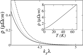
Figure 2: Resistivity in the $x$ direction as a function of $k_{F}\lambda$ where $\lambda$ is the size of the DW. The continuous line corresponds to the elastic case (no magnons), while the dotted and dashed lines were computed including the electron-magnon interaction for T=10 K and 25 K respectively. The anisotropy gap used to obtain these curves was about 116 K (10 meV) and in all cases $J_{K}=0.5$ eV. The inset shows the temperature dependence for $k_{F}\lambda\sim 4.2$.

Fig.2 compares the resistivity along the $x$ direction of a 2D sample for different values of the temperature as a function of $k_{F}\lambda$ with and without including the gapless magnons. The sample size has been taken as $L_{x}$ = 500 $\mu$m and $L_{y}$ = 50 $\mu$m, and $N\sim 3000$. Such a large number of DW are not expected to be naturally pesent in magnetic layers down to arbitrarily low temperatures. However, the interesting nanolayers for spintronics and device applications should present DW at much lower temperatures, and such a number is achieved by experimental techniques down to 2 Ksample . If one considers the typical electronic densities, in the range from 10¹⁵ to 10²⁰ cm^-2, in layers, the DW sizes shown in Fig.2 range from a few Å, to several tenths of Å, consistent with what is also observed in experimentssample .

One sees that an observable increase in the resistivity results for most values of $k_{F}\lambda$, as expected due to the localized character of the gapless magnons. What is notable here, is that even at a temperature of 10 K the effect can be quite observable, while the usual gapped magnons considered in most of the literature would, in this case, affect the results only for temperatures larger than about $116$ K (the anisotropy gap). As a final remark, we would like to point out that these effects can be experimentally checked by measuring the magnetoresitance related to fields higher than the critical DW field. This eliminates scattering processes as phonons or non-magnetic impurities from the background, as it is known. If the remaining resistivity shows a temperature dependence consistent with a magnon bath for temperatures considerably lower than the anisotropy gap, this will strongly suggest the presence of the gapless magnons.

In closing, we have found that, contrary to the case in 1D and to common belief, the magnetic excitation spectrum of a 2D (single-layer) anisotropic ferromagnet should influence charge transport at considerably low temperatures in spite of the anisotropy. This is due to the existence of one dimensional gapless magnons that can propagate in the domain walls formed as the lowest energy configuration. We have provided a theory to describe how electrons interact with both these magnons and the domain wall. We have presented results showing the effect of these magnons on the transport of electrons through domain walls.

A.V.F. and A.O.C. wish to thank Fundação de Amparo à Pesquisa do Estado de São Paulo (FAPESP) for financial support. P.F.F. and A.O.C. kindly acknowledge partial support from Conselho Nacional de Desenvolvimento Científico e Tecnológico (CNPq).

References

- (1) S. A. Wolf, Science 294, 1488 (2001).
- (2) M. Baibich, et al, Phys. Rev. Lett. 61, 2472 (1988).
- (3) H. Ohno, et al, J. Appl. Lett. 73, 363 (1998); H. Ohno, Science 281, 951 (1998).
- (4) Y. Matsumoto, M. Muramaki, T. Shono, T. Hasegawa, T. Fukumura, M. Kawasaki, P. Ahmet, T. Chikyow, S. Koshihara, H. Koinuma, Science 291, 854 (2001).
- (5) M.E. Flatté and G. Vignale, Appl. Phys. Lett. 78 1273 (2001); G. Vignale and M.E. Flatté, Phys. Rev. Lett. 89 098302 (2002).
- (6) G.R. Taylor, A. Isin, and R.V. Coleman, Phys. Rev. 165, 621 (1968).
- (7) J.F. Gregg, et al, Phys. Rev. Lett. 77, 1580 (1996); P.M. Levy and S. Zhang, Phys. Rev Lett. 79, 5110 (1997).
- (8) M. Feigenson, et al., Phys. Rev. B 67, 134436 (2003); M.K. Mukhopadhyay, et al., cond-mat/0302516 (2003).
- (9) J. Tjon and J. Wright, Phys. Rev. B 15, 3470 (1977).
- (10) T. Matsui, Lett. Math. Phys. 42, 229 (1997); T. Khoma and M. Yamanaka, Phys. Rev. B 65, 104434 (2002).
- (11) J.M. Winter, Phys. Rev. 124, 452 (1961); F.C. Burton, C. R. Acad. Sci. (Paris) 252, 3955 (1961); see also A.A. Thiele, Phys. Rev. B 14, 3130 (1976) and M.S. Swanson, Phys. Rev. B 27, 4421 (1983).
- (12) A. Villares Ferrer, P.F. Farinas, and A.O. Caldeira, unpublished.