Resonant nucleation of spatio-temporal order via parametric modal amplification

Abstract

We investigate, analytically and numerically, the emergence of spatio-temporal order in nonequilibrium scalar field theories. The onset of order is triggered by destabilizing interactions (DIs), which instantaneously change the interacting potential from a single to a double-well, tunable to be either degenerate (SDW) or nondegenerate (ADW). For the SDW case, we observe the emergence of spatio-temporal coherent structures known as oscillons. We show that this emergence is initially synchronized, the result of parametric amplification of the relevant oscillon modes. We also discuss how these ordered structures act as bottlenecks for equipartition. For ADW potentials, we show how the same parametric amplification mechanism may trigger the rapid decay of a metastable state. For a range of temperatures, the decay rates associated with this resonant nucleation can be orders of magnitude larger than those computed by homogeneous nucleation, with time-scales given by a simple power law, $\tau_{\rm RN}\sim[E_{b}/k_{B}T]^{B}$, where $B$ depends weakly on the temperature and $E_{b}/k_{B}T$ is the free-energy barrier of a critical fluctuation.

I Introduction

The emergence of spatio-temporal ordered structures in nonlinear systems is an ideal laboratory for investigating the trend toward complexification observed in nature at the physical, chemical, and biological level walgraef . It is known that localized, or spatially-bound, order emerges in systems which are out of thermodynamic equilibrium, at the expense of growing overall disorder bar-yam . Examples can be found in hydrodynamics, in networks of chemical reactions cross , in phase transitions and critical phenomena phase ; magnets ; degennes , and in living organisms schnerb . For these localized ordered structures to survive, they must interact with an external environment, which maintains nonequilibrium conditions: in general, an isolated nonlinear system will eventually reach equilibrium, maximizing its entropy to the detriment of localized ordered structures.

In other words, if localized ordered structures emerge during the approach to equilibrium of a closed system, they will eventually disappear as energy becomes increasingly equipartitioned amongst the system’s many degrees of freedom. The emergence of localized ordered structures is thus a nonequilibrium phenomenon, usually corresponding to an unequal partitioning of energy: if they are long-lived, they will serve as bottlenecks to equipartition. [An exception occurs for 1d field theories with SDW, where configurations such as kink-antikink pairs correspond to the equilibrium.] Following the pioneering work of Fermi, Pasta, and Ulam in the early 1950s ford , several recent works have investigated the possibility that discrete kink-like structures may act as bottlenecks for equipartition in chains of nonlinear oscillators discrete ; bottlenecks .

In field theory and cosmology, most of the interest on ordered configurations has focused on topological (kinks, vortices, monopoles) rajaraman ; vilenkin or nontopological (nontopological solitons, Q-balls) NTSs static solutions of the equations of motion. Those configurations can be boosted towards each other with a certain velocity and made to interact, to model nonlinear composite particle interactions. A well-known example are 1-dimensional breathers, time-dependent bound states that have been shown to result from interactions of kink-antikink pairs campbell . However, this is not surprising: any two or more static solitonic configurations with short-range attractive interactions can be prepared to generate spatially-bound time-dependent structures digal . This is to be contrasted with the spatially-bound, time-dependent structures of interest here, that emerge spontaneously during the nonlinear evolution of a system. We have recently found such structures in 2+1-dimensional simulations of nonlinear scalar field models gleiser-howell . Such structures were identified with oscillons, long-lived time-dependent localized field configurations that have been previously found deterministically in a variety of physical systems, ranging from field theory models with amplitude-dependent nonlinearities gleiser ; bettinson , vertically vibrated grains umbanhowar , and stellar interiors umurhan .

In this paper, we will examine the emergence of spatially-bound, time-dependent field configurations during the approach to equilibrium of (2+1)-dimensional scalar field models with typical double-well interactions. These interactions are controlled by a tunable external parameter, which can be interpreted as an extra interaction that may be switched on or off at will. In the parlance of Ising magnetic systems, the external interaction may be a spatially-homogeneous magnetic field, ${\cal H}(t)$. We will investigate both the symmetric double-well (SDW) – extending previous results of ref. gleiser-howell – as well as provide new results for the asymmetric case (ADW). The interest in examining both cases stems from the fact that the ensuing dynamics will be quite different: while for the SDW the degeneracy in free energy density dictates that no critical nucleation is possible, this will not be the case for the ADW. In fact, for the SDW we observe the synchronous emergence of long-lived localized configurations (oscillons), which eventually disappear as the system reaches equipartition gleiser-howell . We will argue that these configurations act as bottlenecks for equipartition, concentrating the field’s energy in a narrow band of long-wavelength modes. For the ADW, and with the system initially quenched to the metastable state, the synchronous emergence of oscillons may trigger the nucleation of a critical droplet of the lower free-energy phase, which grows to complete the phase transformation. We will show that, for a range of temperatures, the time-scales associated with this process are orders of magnitude faster than the typical statistical homogeneous nucleation, where a system adiabatically cooled into its metastable phase decays to its lowest free energy phase with typically exponentially-large time scales langer ; domb . In fact, the present treatment, with an “instantaneous” quench (faster than other typical time-scales in the system), and the arbitrarily slow cooling implicit of homogeneous nucleation calculations, represent the two extreme cases of a whole spectrum of possible cooling rates. Since we will argue that the emergence of coherent structures is due to the resonant amplification of parametric excitations of certain field modes, we will refer to this nucleation mechanism as resonant nucleation. Anticipating one of our results, for field models described by amplitude-dependent scalar nonlinearities, resonant nucleation of spatio-temporal order will be relevant whenever the cooling time scale $\tau_{\rm cool}$ is faster than the equilibration time-scale of the longest wavelength in the system, $\tau_{\rm eq}^{0}$. [The superscript “0” is a reminder that often the longest wavelength is associated with the zero mode of the system, which has the slowest relaxation time-scale.] We note that we will always work far from the critical point where, of course, $\tau_{\rm eq}^{0}\rightarrow\infty$. For our recent work on the approach to criticality please see ref. howell .

The paper is organized as follows. In the next section we discuss the general properties of the model (a general Ginzburg-Landau model), the initial conditions, and the numerical implementation of the dynamics. In section 3 we present a mean field (homogeneous Hartree) approximation adequate to describe the system in the presence of small fluctuations about equilibrium. The fact that the homogeneous Hartree approximation breaks down as nonperturbative excitations become progressively more important will provide us with useful information about the emergence of ordered structures. In section 4 we argue that the emergence of spatio-temporal order is a consequence of parametric resonance, induced by the nonlinear coupling between the field’s zero mode – the forcing agent – and smaller-$k$ modes. We also provide entropic arguments in support of the statement that the emergence of coherent spatio-temporal structures delays equipartition of the energy and, thus, the approach to equilibrium. In section 5, we extend our investigation to ADWs. For a range of temperatures [or initial energies, see below], we measure the time scales for the decay of the metastable state as a function of barrier height, contrasting them with those computed from homogeneous nucleation theory. We identify two possible mechanisms for the decay: for small asymmetries, a critical nucleus is produced by the coalescence of two or more oscillons, while for larger asymmetries a single oscillon evolves into a critical nucleus. We show that, for a range of temperatures associated with the presence of oscillons in the system, the time scale associated with the decay obeys a simple power law, $\tau_{\rm RN}\sim[E_{b}/k_{B}T]^{B}$, where $E_{b}/k_{B}T$ is the free-energy barrier of a critical fluctuation, and the exponent $B$ satisfying $\simeq 2.44<B(T)<3.36$. We conclude in section 6 with a summary of our results and outlook for future work.

II The nonlinear model and its implementation

We start by introducing the model we will work with and its statistical and numerical implementation. We consider a (2+1)-dimensional real scalar field (or scalar order parameter) $\phi({\bf x},t)$ evolving under the influence of an on-site potential $V(\phi)$. If the system does not interact with an external bath, the continuum Hamiltonian is conserved and gives the total energy of the system, for a given field configuration,

$$H[\phi]=\int d\,^{2}x\left[\frac{1}{2}(\partial_{t}\phi)^{2}+\frac{1}{2}(\nabla\phi)^{2}+V(\phi)\right],$$ (1)

where

$$V(\phi)=\frac{m^{2}}{2}\phi^{2}-\frac{\alpha}{3}\phi^{3}+\frac{\lambda}{8}\phi^{4}$$ (2)

is the potential energy density. The parameters $m$,$\alpha$, and $\lambda$ are positive definite and temperature independent. Before we go any further, a note on our choice of potential. One could as easily have chosen a typical Ginzburg-Landau (GL) potential, $V(\phi)=-\frac{a}{2}\phi^{2}+\frac{\lambda}{8}\phi^{4}-{\cal H}(t)\phi$, with ${\cal H}(t)$ an external homogeneous magnetic field. The GL potential can be transformed into the potential of eq. 2 by a field shift, $\phi^{\prime}=\phi+C({\cal H};a,\lambda)$, where $C$ is the solution of the cubic equation $C^{3}-2\frac{a}{\lambda}C+\frac{2H}{\lambda}=0$, $\alpha=\frac{3}{2}\lambda C$, and $m^{2}=-a+\frac{3}{2}C^{2}\lambda$. We chose the potential of eq. 2 for convenience. Our control parameter is $\alpha$. We note that when $\alpha=0$ the potential is an anharmonic single well. In this case, there are no spinodal instabilities. (By spinodal instabilities we mean $V^{\prime\prime}(\phi)<0$ for certain values of $\phi$, which may result in the unstable growth of modes.) When $\alpha\geq 3/2$ (in scaled units, see below) the potential can assume a typical double-well shape [SDW for equality and ADW for $\alpha>3/2$], and spinodal instabilities are possible. We will thus refer to the interactions modeled by $\alpha$ as destabilizing interactions (DIs). Changing $\alpha$ from an initial value of zero to a finite positive value can also be thought of as an “instantaneous” quench: the system, initially prepared in a single well, is “tossed” into a double-well potential within a time-scale much faster than any equilibration time-scale for longer wavelengths in the system, those with $k^{2}\lesssim 2\pi V^{\prime\prime}(\phi=0)$, where $k$ is the mode’s wave number. We will say more about this later on.

It is helpful to introduce the dimensionless variables $\phi^{\prime}=\phi\,\sqrt{\lambda}/m$, $x^{\prime}=xm$, $t^{\prime}=tm$, and $\alpha^{\prime}=\alpha/(m\sqrt{\lambda})$ (henceforth dropping the primes). When $\alpha\equiv\alpha_{c}=3/2$ the two minima are degenerate (SDW). If $\alpha\neq 0$, the ${\cal Z}_{2}$ symmetry is explicitly broken. We will only be concerned here with the cases modeled by $\alpha\geq\alpha_{c}$. For $\alpha>\alpha_{c}$ the minimum at $\phi=0$ becomes the local (or metastable) minimum (ADW) and $\phi_{+}=\alpha+\sqrt{\alpha^{2}-2}$ is the global minimum.

II.1 Statistical Implementation and Initial Conditions

A statistical description of the state of the system is given by a set of time-dependent observables $\{\langle O^{(1)}(t)\rangle,\langle O^{(2)}(t)\rangle,\ldots\}$, each one calculated as an ensemble average over $N$ realizations, or microstates. For example,

$$\langle O^{(1)}(t)\rangle=N^{-1}\sum_{i=1}^{N}O^{(1)}_{i}(t).$$ (3)

In most cases, an observable within a particular microstate is itself an average over the area of the system, such as the average value of the field $\phi_{i}(t)=A^{-1}\int_{A}\!d\,^{2}x\,\phi_{i}({\bf x},t)$ for the particular microstate $i$. Most of the observables considered will have this “double” averaging. Such is the case for $\langle\phi(t)\rangle$, $\langle\pi(t)\rangle$ (the field’s conjugate momentum), and the corresponding hierarchy of correlation functions. It will be noted when this is not the case, particularly when quantities are no longer assumed to be translationally invariant, such as those describing localized configurations.

We prepare the field such that it is in thermal equilibrium at temperature $T$ in the single-well ($\alpha=0$) potential at some time prior to the quench at $t=0$, when $\alpha$ is set to a nonzero value. When one is faced with a nonlinear equation of motion such as eq. 4 below, the thermal probability distribution for $\phi({\bf x},0)$ cannot be obtained exactly. To generate the initial conditions for each of the microstates in the ensemble, we instead couple the field in the single-well potential to a heat bath via a generalized Langevin equation with additive noise,

$$\ddot{\phi}+\gamma\dot{\phi}-\nabla^{2}\phi=-\phi-\frac{1}{2}\phi^{3}+\xi,$$ (4)

where the viscosity coefficient $\gamma$ is related to the stochastic force of zero mean $\xi({\bf x},t)$ by the fluctuation-dissipation relation,

$$\langle\xi({\bf x},t)\,\xi({\bf x^{\prime}},t^{\prime})\rangle=2\gamma T\,\delta^{2}({\bf x}-{\bf x^{\prime}})\,\delta(t-t^{\prime}).$$ (5)

Eq. 5 defines the two-point correlation function of the stochastic force, assumed here to be Markovian. Since this force will only be used during the preparation of the initial thermal state – after the quench the coupling with the bath is turned off ($\gamma\rightarrow 0$) – this assumption is sufficient. [However, it would be quite interesting to examine the effects of multiplicative noise in the nonequilibrium dynamics of this system when the contact with the thermal bath is kept throughout its evolution. [The role of multiplicative noise on the onset of synchronization in 1+1-dimensional fields has been recently investigated by Munõz and Pastor-Satorras munoz .] We note that even though we are preparing each microstate in an initial thermal state, there is a one to one correspondence between the temperature and the average energy of the field. In fact, we can refer to the ensemble prepared as above as a microcanonical ensemble, since each microstate has energy $E\pm\delta E$, where $\delta E/E<10^{-3}$. Such numerical accuracy in energy matches that obtained with other methods used preparing the initial state, including the popular Monte Carlo sampling. It simply expresses the fact that, for large enough lattices that approach the thermodynamic limit, there is an equivalence between canonical and microcanonical ensembles chandler .

II.2 Numerical Implementation

The full evolution of the scalar field for each microstate is simulated using a staggered leapfrog integration of the equation of motion. It is implemented on a square lattice with periodic boundary conditions. Integrations are performed with $\Delta x=0.2$ and $\Delta t=0.02$ with 1024 lattice sites per side. The field is then defined over an area with sides of length $L=204.8$. The leapfrog scheme replaces second-order derivatives with finite-difference expressions that are accurate to ${\cal O}(\Delta x^{2},\Delta t^{2})$. The lattice spacing and system size are chosen so that computations can be carried out in a timely manner, while the numerical values of any observables and their corresponding continuum values are in good agreement. For example, after the quench, the energy in this closed system is conserved by more than 1 part in $10^{3}$. Results are independent of lattice size, provided large enough lattices are used. Finally, all of the observables are then averaged over an ensemble of $N=100$ microstates.

III Dynamics within the perturbative realm: Homogeneous Hartree Approximation

III.1 Setting up the initial configuration

We start our investigation using a familiar perturbative method, the leading order or Homogeneous Hartree Approximation (HHA). An excellent account can be found in bonini , where successive truncations within the hierarchy of correlation functions were used to simplify the equation of motion, all the while capturing the essential aspects of the dynamics. We will borrow many of the same methods and notation found in this reference. The HHA assumes that the statistical distribution of the fluctuations in the field and its momentum remain Gaussian throughout the evolution of the system. We will see that this is indeed an excellent approximation in the following cases: i) just prior to the quench (that is, the initial state of the field in a single well) for all temperatures considered; ii) at all times after the quench when the temperature is low; iii) at very early times after the quench when the temperature is high. We start by considering the system before the quench is implemented ($\alpha=0$), that is, the dynamics with the potential $V(\phi)=\frac{1}{2}\phi^{2}+\frac{1}{8}\phi^{4}$ boyanovsky:03 .

A simple way to implement the HHA in this situation is to factor the cubic term in eq. 4 as $\phi^{3}({\bf x},t)\to 3\langle\phi^{2}\rangle\phi({\bf x},t)$, where $\langle\phi^{2}\rangle$ is the translationally invariant mean-square variance of the field. Since the field is in thermal equilibrium, $\langle\phi^{2}\rangle$ is time-independent. In this approximation, the equation of motion becomes linear,

$$\ddot{\phi}-\nabla^{2}\phi=-\left(1+\frac{3}{2}\langle\phi^{2}\rangle\right)\phi.$$ (6)

The Fourier transform of the field is a complex quantity given by

$$\bar{\phi}({\bf k},t)=\frac{1}{(2\pi)^{2}}\int\!d\,^{2}x\,\phi({\bf x},t)\,e^{i{\bf k\cdot x}}.$$ (7)

The corresponding equation of motion for $\bar{\phi}({\bf k},t)$ in $k$-space is [with $k=(k_{x}^{2}+k_{y}^{2})^{1/2}$]

$$\ddot{\bar{\phi}}=-\omega^{2}(k)\bar{\phi},$$ (8)

with the effective frequency squared

$$\omega^{2}(k)=k^{2}+1+\frac{3}{2}\langle\phi^{2}\rangle=k^{2}+m_{H}^{2}.$$ (9)

We have introduced the Hartree mass $m_{H}^{2}=1+\frac{3}{2}\langle\phi^{2}\rangle$. Notice that when there are fluctuations in this field ($\langle\phi^{2}\rangle>0$) the effective Hartree mass is greater than the “bare” mass ($m^{2}=1$) given by the potential in eq. 2. In this approximation, the modes evolve independently of one another, just as they would in a linear truncation of the equation of motion, only now each interacts with the homogeneous mean-field background. A higher-order approximation is needed, however, to implement direct scattering between different modes.

If the system is in thermal equilibrium, the momentum modes in $k$-space will satisfy

$$\langle|\bar{\pi}({\bf k})|^{2}\rangle=T.$$ (10)

It then follows from eq. 8 that the corresponding power spectrum for the field is

$$\langle|\bar{\phi}({\bf k})|^{2}\rangle=\frac{T}{k^{2}+m_{H}^{2}}.$$ (11)

To obtain the equilibrium quantity $\langle\bar{\phi}^{2}\rangle$, one integrates eq. 11 over the entire $k$-space and divides by the area. (Equivalently, one can integrate the corresponding two-point correlation function over $x$-space to obtain $\langle\phi^{2}\rangle$, since Parseval’s theorem guarantees that the two quantities are the same.) One must be careful here, since the lattice results depend logarithmically on the ultraviolet cutoff (lattice-spacing). We refer the reader to ref. borrill , where a method is provided to handle such dependence perturbatively.

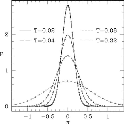
Figure 1: The probability distribution of $\pi$ for various temperatures. The continuous lines are the theoretical predictions given by eq. 12.

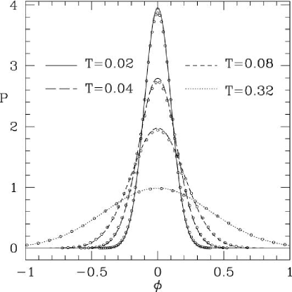
Figure 2: The probability distribution of $\phi$ for various temperatures. The continuous lines are the approximations given by eq. 13.

In figures 1 and 2 we show the probability distributions for the initial state of the field and its momentum for various temperatures. These distributions are obtained numerically by collecting the values of $\pi({\bf x},0)$ and $\phi({\bf x},0)$ of every microstate into bins of width $\Delta\pi=\Delta\phi=0.01$, and then normalizing so that the sum over each distribution is unity. Not all data points are shown, making these figures more readable. Also shown are the Gaussian probability distributions (solid lines) that are predicted from the Boltzmann-Gibbs formalism,

$$P(\pi)= \frac{1}{\sqrt{2\pi T}}e^{-\frac{\pi^{2}}{2T}}$$ (12)

$$P(\phi)= \frac{1}{\sqrt{2\pi aT}}e^{-\frac{\phi^{2}}{2aT}}.$$ (13)

The fitting parameter $a\simeq 0.51$ is obtained by comparing the area (and ensemble)-averaged two-point corrrelation function of $\phi$. The variance in figure 2, $\langle\phi^{2}\rangle$, can be fitted linearly, $\langle\phi^{2}\rangle=aT$. The agreement between the numerical results and the theoretical predictions confirms the accuracy of the lattice dynamics and the applicability of the HHA for low enough temperatures. The probability distribution of $\pi({\bf x},0)$ is exact, while that of $\phi({\bf x},0)$ is indeed close to Gaussian for the temperatures considered. We also show, in figure 3, the power spectrum of the field modes, $\langle|{\bar{\phi}}({\bf k},0)|^{2}\rangle$, and compare it with the prediction from eq. 11, valid for the HHA.

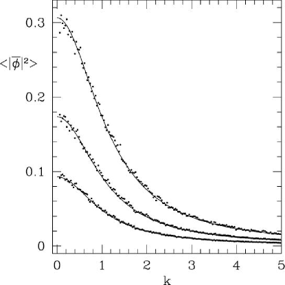
Figure 3: The power spectrum $\langle|\bar{\phi}(k)|^{2}\rangle$ for temperatures $T$=0.1, 0.2, and 0.4. The solid lines are the approximations given by eq. 11.

III.2 Dynamical evolution and breakdown of Hartree approximation

In this subsection we examine the dynamics of the field after the quench. We will limit our investigation to the case where $\alpha\rightarrow\alpha_{c}=3/2$ at $t=0$, that is, the potential is switched from a single well to a SDW. The dynamics for ADW potentials will be examined in section 5.

At $t=0$ the coupling to the bath is set to zero, and the dynamics is thus conservative thereafter. The system is closed, and can be described by a microcanonical ensemble of energy $\langle E\rangle\pm\delta E$, where $\delta E/\langle E\rangle\ll 1$. As we remarked before, for large enough systems in equilibrium, as is the case here for $t<0$, a description with fixed $E$ is equivalent to one with fixed $T$. We will use this initial temperature to characterize the system. It is interesting to note that in the thermodynamic limit, an instantaneous quench to any positive value of $\alpha$ will not change the energy of the system. The field is initially symmetric in its distribution and the quench introduces an odd term into the Hamiltonian. Instead, the energy is redistributed between its kinetic, gradient, and potential parts, and as a result the final equilibrium temperature will necessarily differ from the initial temperature. In this investigation, however, this change is always less than $0.15$ percent. For open systems, where the system remains in contact with a heat bath, we refer the reader to ref. gleiser-howell .

Due to the initial thermal distribution, defined entirely by the temperature $T$, the sudden introduction of the cubic term into the potential actually has a minor effect on most of the field. In general, there is little net change in the forces present throughout the system, since the curvature of the single- and double-well potentials are the same at $\phi=0$ and the majority of the field is indeed close to this value (see figure 2). That is, the linear equation of motion remains unchanged for the small-amplitude fluctuations that represent the peak of the field’s probability distribution. The few locations where the field is more responsive to the perturbation correspond to regions with relatively large absolute values of $\phi$. These values define the tails of the probability distribution. The new nonlinear term present in the potential breaks the symmetry in the equation of motion, and this second-order effect causes larger-amplitude field fluctuations with negative (positive) values to experience a larger (smaller) restoring force than before. Overall, a net positive force is imposed on the symmetrically prepared field and, as a consequence, its average starts at $\langle\phi\rangle=0$ and then begins to move toward $\phi_{\rm max}$, the maximum of the potential barrier between the two states.

We will see that $\langle\phi(t)\rangle$ is initially driven more out of equilibrium than all of the fluctuations about it. This is not surprising, as longer wavelength modes have longer relaxation time-scales langer . It is natural, then, to distinguish the dynamics of the two from each other. First, define $\phi_{\rm ave}(t)\equiv\langle\phi(t)\rangle$ and let $\delta\phi({\bf x},t)$ represent the fluctuations about this average. Then,

$$\phi({\bf x},t)=\phi_{\rm ave}(t)+\delta\phi({\bf x},t),$$ (14)

where $\langle\delta\phi({\bf x},t)\rangle=0$ by definition. In the HHA, one assumes that these fluctuations and their momenta remain Gaussian in their distribution. One then obtains an equation of motion for $\phi_{\rm ave}(t)$,

$$\ddot{\phi}_{\rm ave}=-\frac{\partial V_{\rm eff}}{\partial\phi_{\rm ave}}~{},$$ (15)

where we have introduced the effective potential for $\phi_{\rm ave}$,

$$V_{\rm eff}\left(\phi_{\rm ave},\langle\delta\phi^{2}\rangle\right)=\left[1-m_{\rm H}^{2}(t)\right]\phi_{\rm ave}+\frac{1}{2}\,m_{\rm H}^{2}(t)\,\phi_{\rm ave}^{2}-\frac{\alpha_{\rm c}}{3}\,\phi_{\rm ave}^{3}+\frac{1}{8}\,\phi_{\rm ave}^{4},$$ (16)

that depends explicitly on the mean-square variance of the fluctuations through the time-dependent Hartree mass $m_{\rm H}^{2}(t)=1+\frac{3}{2}\langle\delta\phi^{2}(t)\rangle$.

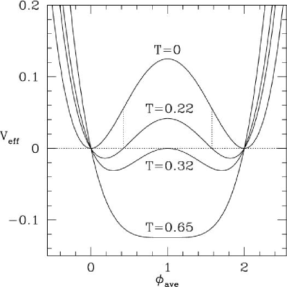
Figure 4: The effective potential for $\phi_{\rm ave}$, just after the quench, for various initial temperatures $T$. The two vertical lines correspond to the inflection points of the bare ($T=0$) potential. They are also the turning points for the potential at $T\simeq 0.22$. At $T\simeq 0.32$ the turning point is $\phi_{\rm max}$.

$V_{\rm eff}$ at $t=0$ is shown in figure 4 for various temperatures. For sufficiently low initial temperatures (how low will become clear soon), $\phi_{\rm ave}(t)$ will oscillate about the LHS minimum of the effective potential, $\phi_{-}=1-\sqrt{1-3\langle\delta\phi^{2}\rangle}$. It will then begin to relinquish its energy to higher modes through nonlinear scattering, and its amplitude will decay. It is possible, then, to approximately bound this region of oscillation from the set of turning points for $\phi_{\rm ave}(t)$ [with $\langle\delta\phi^{2}\rangle$ retaining its $t=0$ value],

$$\phi^{\rm tp}_{\rm ave}=\left\{0,\,1\pm\sqrt{1-6\langle\delta\phi^{2}\rangle},\,2\right\}.$$ (17)

These values give the location of $\phi_{\rm ave}(t)$ where $V_{\rm eff}=0$, and $\pi_{\rm ave}(t)=\partial_{t}\phi_{\rm ave}(t)$ vanishes. When $\langle\delta\phi^{2}\rangle<1/6$ there are four such turning points because of the symmetry about $\phi_{\rm max}$. The primary region of interest is when $\phi^{\rm tp}_{\rm ave}\simeq\phi_{\rm inf(-)}$, when fluctuations begin to probe the spinodal region of $V_{\rm eff}$. By using eq. 17, we can predict that $\phi_{\rm ave}(t)$ will probe this region when $\langle\delta\phi^{2}\rangle=1/9$, or $T\simeq 0.22$. Clearly, this is also where the leading-order Hartree approximation fails.

It is interesting to consider also the case when $\langle\delta\phi^{2}\rangle=1/3$, or $T\simeq 0.65$. There are only two turning points for $\phi_{\rm ave}$, since $V_{\rm eff}$ is now a single-well potential symmetric about $\phi=\phi_{\rm max}$. The fluctuations are large enough that the local maximum in the bare potential has little influence in the dynamics, and $\phi_{\rm ave}=\phi_{\rm max}$. The fluctuations actually probe beyond both minima of the potential. This case is similar to the phenomena of symmetry restoration in continuous phase transitions, and so in this context $T\simeq 0.65$ would be considered the critical temperature, $T_{c}$. For all higher temperatures, $\phi_{\rm ave}=\phi_{\rm max}$ phase ; gleiser-mix . In this work, we are only concerned with temperatures well below $T_{c}$, in fact below $T=0.32$, where $\phi^{\rm tp}_{\rm ave}=\phi_{\rm max}$ (see figure 4).

In order to further quantify the dynamics in the HHA, we derive the set of differential equations for the time evolution of the coupled two-point correlation functions. We define the translationally invariant quantities

$$G_{\phi\phi}({\bf x-y},t) = \langle\delta\phi({\bf x},t)\delta\phi({\bf y},t)\rangle$$

$$G_{\pi\pi}({\bf x-y},t) = \langle\delta\pi({\bf x},t)\delta\pi({\bf y},t)\rangle$$ (18)

$$G_{\pi\phi}({\bf x-y},t) = \frac{1}{2}\left(\langle\delta\pi({\bf x},t)\delta\phi({\bf y},t)\rangle+\langle\delta\phi({\bf x},t)\delta\pi({\bf y},t)\rangle\right).$$

Upon taking the time-derivative of each expression, the equations of motion can then equivalently be written in $k$-space. They are

$$\dot{G}_{\phi\phi}(k,t) = 2G_{\pi\phi}(k,t)$$

$$\dot{G}_{\pi\pi}(k,t) = -2\bar{\omega}^{2}G_{\pi\phi}(k,t)$$ (19)

$$\dot{G}_{\pi\phi}(k,t) = G_{\pi\pi}(k,t)-\bar{\omega}^{2}G_{\phi\phi}(k,t)~{},$$

where ${\bar{\omega}}^{2}(k)=k^{2}+V_{\rm eff}^{\prime\prime}\left[\phi_{\rm ave}(t),\langle\delta{\bar{\phi}}^{2}(t)\rangle\right]$.

These equations, coupled with

$$\dot{\pi}_{\rm ave} = -\frac{\partial V_{\rm eff}}{\partial\phi_{\rm ave}}$$ (20)

$$\dot{\phi}_{\rm ave} = \pi_{\rm ave},$$

give the full dynamics of $\pi_{\rm ave}(t)$ and $\phi_{\rm ave}(t)$ and their corresponding two-point correlation functions $\langle\delta\pi^{2}({\bf k},t)\rangle$ and $\langle\delta\phi^{2}({\bf k},t)\rangle$ in the HHA. These two groups of expressions are likewise coupled through the quantities $\langle\bar{\delta\phi}^{2}(t)\rangle=\langle\delta\phi^{2}(t)\rangle$ and $\phi_{\rm ave}(t)$. The initial conditions are given by eqs. 10, 11, and also $\pi_{\rm ave}(0)=\phi_{\rm ave}(0)=0$.

These five first-order equations were solved numerically using a fourth-order Runge-Kutta algorithm. The same lattice spacing from the leap-frog algorithm was used. The calculation of $\langle\bar{\delta\phi}^{2}(t)\rangle$ is obtained by numerically averaging the radial function $G_{\phi\phi}(k,t)$ over the disk in $k$-space with radius $k^{2}=k_{x}^{2}+k_{y}^{2}$, bounded by $k_{\rm max}=\pi/\Delta x$. There is a slight discrepancy between the area of rectangular phase space used in the two-dimensional numerical integrations and the circular phase space used in this method. In light of the previous discussion regarding the dependence of the correlation functions on the lattice spacing, this difference could possibly introduce error in the calculations of $\langle\bar{\delta\phi}^{2}(t)\rangle$. To compensate for the smaller area used in the HHA, the initial conditions for $\langle\bar{\delta\phi}^{2}(k,0)\rangle$, given by eq. 11, are multiplied by a normalization factor of 1.041 so that the radial integration gives the expected average $\langle\bar{\delta\phi}^{2}\rangle=aT$ at $t=0$. The results will confirm the validity of this normalization method.

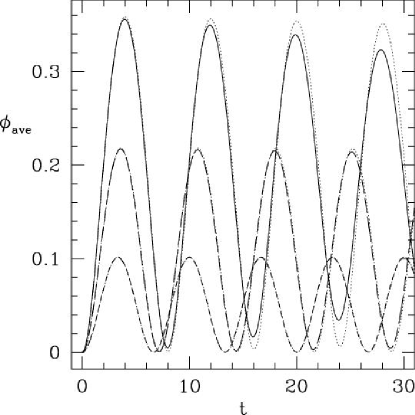
Figure 5: Numerical evolution of $\phi_{\rm ave}(t)$ compared to that obtained through the Hartree approximation, for various initial temperatures. Shown are $T=0.06$ (short dash), $T=0.12$ (long dash), and $T=0.18$ (solid), as well as the corresponding Hartree approximations (dotted).

Shown in figure 5 is the numerical time evolution of $\phi_{\rm ave}(t)$ compared to that obtained through the HHA, for various initial temperatures. The agreement is clearly excellent at lower temperatures, where $\langle\phi_{\rm ave}(t)\rangle$ undergoes almost-linear oscillations about the minimum of $V_{\rm eff}$: there is very little scattering between modes. At $T\simeq 0.18$ scattering begins to take place, allowing for a slow transfer of energy from low-$k$ modes to higher-$k$ modes not accounted for in the HHA. We will soon show that this is also the temperature where the synchronous emergence of spatio-temporal order begins to take place. Notice also the dependence of the oscillation frequencies on the initial thermalization temperature.

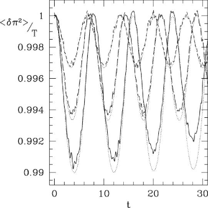
Figure 6: The numerical evolution of $\langle\pi^{2}(t)\rangle/T$ compared to that obtained through the Hartree approximation, for various initial temperatures. Shown are $T=0.06$ (short dash), $T=0.12$ (long dash), and $T=0.18$ (solid), as well as the corresponding Hartree approximations (dotted).

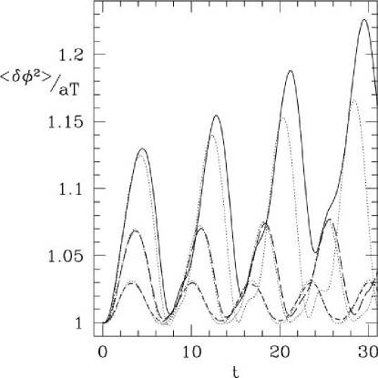
Figure 7: The numerical evolution of $\langle\phi^{2}(t)\rangle/aT$ compared to that obtained through the Hartree approximation, for various initial temperatures. Shown are $T=0.06$ (short dash), $T=0.12$ (long dash), and $T=0.18$ (solid), as well as the corresponding Hartree approximations (dotted).

Figures 6 and 7 compare the numerical time-evolution of $\langle\delta\pi^{2}(t)\rangle$ and $\langle\delta\phi^{2}(t)\rangle$ with the corresponding HHA predictions. The quantities are normalized to unity at $t=0$ through $\langle\pi^{2}\rangle=T$ and $\langle\phi^{2}\rangle=aT$, respectively. The agreement is again excellent at lower temperatures. At $T=0.18$, however, it is evident that energy is being fed into the fluctuations of the field. The full numerical evolution depicts the amplitude of oscillation of $\langle\delta\pi^{2}(t)\rangle$ decreasing at a rate larger than that predicted by the HHA. Similarly, the amplitude of oscillation of $\langle\delta\phi^{2}(t)\rangle$ increases at a larger rate. Again, this discrepancy is due primarily from the approximation’s inability to account for direct scattering between modes.

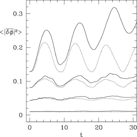
Figure 8: The numerical evolution of the two-point correlation function $\langle|\bar{\phi}(k,t)|^{2}\rangle$ for various values of $k$. Also shown are the results from the corresponding Hartree approximation (dotted lines). The initial temperature is $T=0.22$. The amplitudes decrease for increasing $k$. Shown, from the top down, are $k$=0.75, 1.25, 2.0, and 4.75.

In figure 8 we show the transfer of energy between different $k$-modes. Displayed is the time evolution of $\langle|\bar{\delta\phi}(k,t)|^{2}\rangle$ for indicative values of $k$. The initial thermalization temperature is $T=0.22$, corresponding to the value in which the majority of the field probes the spinodal region (cf. section IV). This is well above the region of temperatures in which the HHA is accurate. From the figure it is clear that scattering between low $k$ modes modes is taking place. The approximation is only accurate for shorter wavelength modes, due to the fact that they remain in equilibrium even after the quench. The breakdown of the HHA at longer wavelengths implies that important nonlinear effects are strongly influencing the behavior of the field. In the next section we investigate the emerging dynamics of these modes.

IV Emergence of spatio-temporal order in a SDW model

IV.1 Beyond the Homogeneous Hartree Approximation

The results of the last section should have made it clear that at high temperatures nonlinear scattering leads to an efficient energy transfer between modes. This energy transfer will eventually lead to the thermalization of the field in the SDW potential. As predicted by the HHA, at $T\gtrsim 0.18$ there is consistent energy transfer from the zero-mode to these higher-$k$ modes. At these initial temperatures, $\phi_{\rm ave}(t)$ undergoes damped oscillations about its effective minimum. For $T=0.22$, the amplitudes of these oscillations are large enough that $\phi_{\rm ave}(t)$ just crosses the inflection point of the bare potential: roughly half of the field probes the spinodal region.

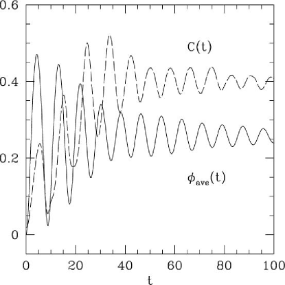
Figure 9: $\phi_{\rm ave}(t)$ (solid line) and $C(t)$ (dashed line) for $T=0.22$.

Figure 9 illustrates the transfer of energy from $\phi_{\rm ave}(t)$ to the fluctuations $\langle\delta\phi^{2}(t)\rangle$ for $T=0.22$. The quantity

$$C(t)\equiv\frac{\langle\delta\phi^{2}(t)\rangle-aT}{aT}$$ (21)

is introduced so that a visual comparison can be made between these two components of the field. Notice the correlation between the decaying amplitude of oscillation for $\phi_{\rm ave}(t)$ and the increasing amplitude of the fluctuations. At $t\simeq 60$ most of this energy transfer is complete, after which time the two quantities display smaller oscillations that are almost exactly out of phase with each other. For earlier times, $0\leq t\leq 60$, a highly nonlinear scattering process occurs, as the zero-mode of the field pumps its energy into its neighboring small-$k$ modes.

Figure 10 shows the numerical time-evolution of $\langle|\bar{\delta\phi}(k,t)|^{2}\rangle$ for $0\leq k\leq 4$ and $0\leq t\leq 60$, at $T=0.22$. First, notice that growth occurs mainly for modes with $0\leq k\leq 0.5$. Their maximum amplitude reaches a value that is up to 15 times greater than at $t=0$. The oscillations then begin to decay and, for $t>60$ (discussed later), the amplitudes of the modes take on a constant value, albeit still many times larger than their initial value. It is also apparent that for the time interval shown modes with $k>1$ are nearly time-independent, maintaining their initial thermal spectrum given by eq. 11. This is true of all large-$k$ modes present in the numerical simulation, up to $|k|_{\rm max}\simeq 15.7$, which also indicates that the lattice spacing used has no effect on the emerging dynamics of the system.

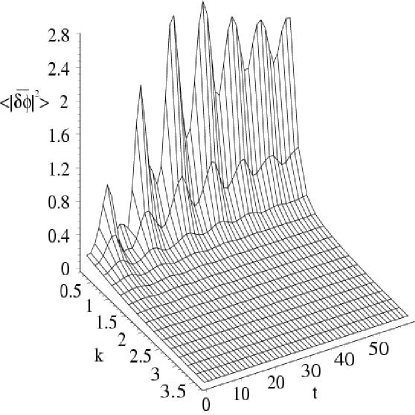
Figure 10: The spectrum of the field for times $0\leq t\leq 60$.

We would now like to search for possible spatio-temporal ordering during the field’s approach to equilibrium. However, due to the noisy initial conditions, it is quite difficult to extract information about any emergent pattern, be it spatial and/or temporal. An added advantage to having an analytical expression for the initial thermal spectrum for all temperatures of interest (cf. eq. 11) should be clear: a Wiener filter is extremely successful at removing undesirable noise whenever its spectrum is known, all the while maximally preserving the nonperturbative fluctuations that emerge numericalrecipes .

IV.2 Synchronous emergence of spatio-temporal order

With the filtered field, one can catalog and track the location of all local extrema in the system at each instant in time and for all initial temperatures. To distinguish the large-amplitude fluctuations from the long-wavelength thermal noise that is also passed by the filter, only the values of these extrema that are greater than the characteristic amplitude of the noise, $\delta\phi^{2}({\bf x},t)>aT$, are considered. With ample sorting, a library is compiled containing the description of every large-amplitude fluctuation present during the entire evolution of the system (the maximum time for the simulations is $t_{\rm max}=2000$). For each fluctuation the following attributes are recorded: its core location ${\bf x}_{\rm f}$, nucleation time $t_{\rm nuc}$, core amplitude $\phi_{\rm a}$ (measured at ${\bf x}_{\rm f}$), radius $R$ (measured at half maximum), its total number of oscillations $N_{\rm osc}$, the period of each oscillation ${\cal T}_{N}$, and its lifetime $\tau$.

Each of these attributes is time-dependent, with the exception of $N_{\rm osc}$ and $\tau$. Almost every large-amplitude fluctuation oscillates anharmonically about the background value $\phi_{\rm ave}(t)$, which is recognized by the fact that most of them reappear at approximately the same location with regular frequency. Therefore, in general it is possible to establish the relationship $N_{\rm osc}=\tau/{\cal T}$, where ${\cal T}\equiv\langle{\cal T}_{N}\rangle$ is the average period of oscillation. The set of observables is further reduced by averaging ${\bf x}_{f}$, $\phi_{\rm a}$, and $R$ over their corresponding values at the maximum of each oscillation for the lifetime of the fluctuation. Other than the nucleation time $t_{\rm nuc}$, each attribute is now time-independent. Hereafter, we will omit the $\langle\cdots\rangle$ notation and assume that these values are indeed averages.

With this information, a probability distribution function for the large-amplitude fluctuations is obtained for each initial temperature. This function, denoted as $F_{T}({\bf x}_{f},t_{\rm nuc},\phi_{\rm a},R,{\cal T},\tau)$, can be used to calculate averages over any of its variables. Similarly, one can integrate this function over a subset of variables to obtain a reduced distribution. In all cases, $F_{T}$ is normalized so that a numerical integration over all variables evaluates to unity. The bin widths of each variable (as any one variable of $F_{T}$ will be visualized as a histogram) will be specified below.

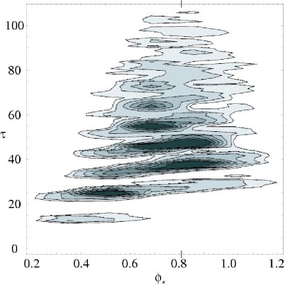
Figure 11: The probability distribution for the amplitude and lifetime of all fluctuations accounted for early in the evolution ($t<100$). The darkest regions correspond to the most abundant fluctuations (probability $f=0.07$), with each lighter region then descending in intervals $\Delta f=0.01$.

For the moment, we focus our attention on the characteristics of fluctuations early in the evolution of the field, $0\leq t\leq 100$, and at an initial temperature $T=0.22$. The quantity

$$f_{T}(\phi_{\rm a},\tau)=\int_{A}\!\!d\,^{2}x_{\rm f}\int_{0}^{100}\!\!\!dt_{\rm nuc}\int_{0}^{L/2}\!\!\!dR\int_{0}^{t_{\rm max}}\!\!\!d{\cal T}\,\,F_{T}$$ (22)

gives the reduced distribution function for the core amplitude and lifetime, and is shown in figure 11. The bin widths are $\Delta\phi_{\rm a}=0.05$ and $\Delta\tau=1$. The darkest regions in the figure correspond to the most probable fluctuations. Particularly noticeable is that fluctuations with core amplitudes $0.55\leq\phi_{\rm a}\leq 1.0$ and lifetimes $35\leq\tau\leq 65$ dominate the distribution. One can also see that fluctuations with small amplitudes $0.2\leq\phi_{\rm a}\leq 0.5$ have mostly short lifetimes. There is a group of fluctuations, however, that have lifetimes $80\leq\tau\leq 100$ and thus remain present in the system for substantially long periods of time. In addition, their core amplitudes are confined to a narrower region $0.7\lesssim\phi_{\rm a}\lesssim 0.9$. Also marked on the horizontal axes is the location $\phi_{\rm a}=0.81$, which corresponds to the difference between the local maximum and the left minimum of the effective potential for $T=0.22$, given by eq. 16. It follows that these long-lived oscillatory fluctuations have large enough amplitudes that their cores probe a narrow region centered about $\phi_{\rm max}$. In fact, the large majority of long-lived fluctuations probe beyond the inflection point of $V_{\rm eff}$ at $\phi_{\rm inf(-)}\simeq 0.4$. They are clearly nonperturbative in nature and would not be seen within the HHA.

In figure 12 we show a sequence of snapshots of the filtered field within the time interval $21.0\leq t\leq 29.4$. There are several features to be noted. [Clearly, they are more striking with a full animation. We invite the reader to view simulations in ref. website .] First, large-amplitude fluctuations seem to be of similar size (spatially-bound configurations) and spread throughout the lattice. Second, they emerge in near synchrony. As we will see below, this global ordering persists for the first few oscillation cycles. Third, as can be seen from figure 11, these configurations can be quite long-lived.

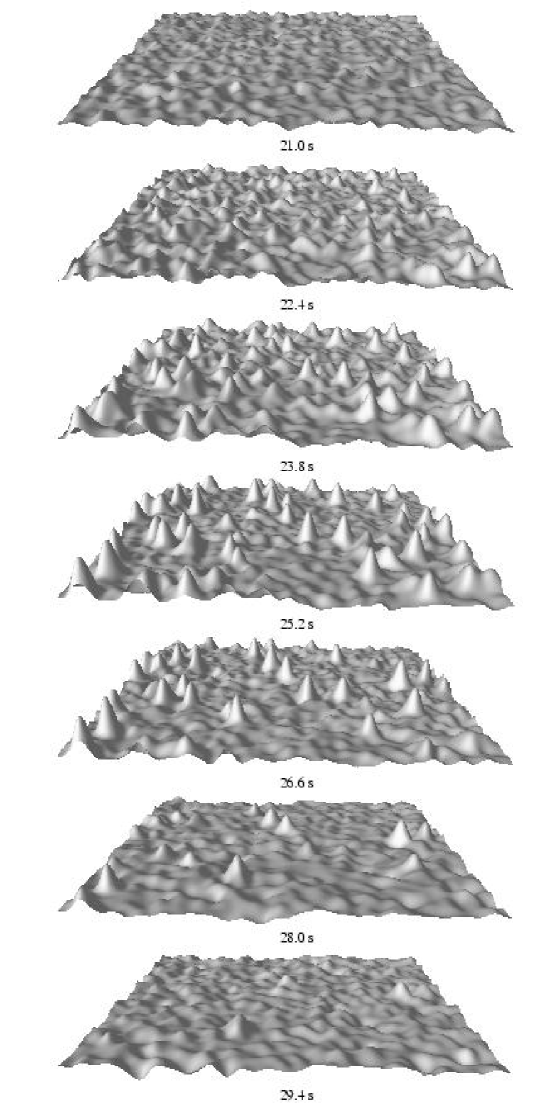
Figure 12: Snapshots displaying the synchronous emergence of oscillons in the two-dimensional field. The initial temperature is $T=0.22$. Simulations can be viewed in ref. website .

We identify these spatially-bound, long-lived configurations with oscillons, which have been originally found as deterministic solutions of models with amplitude-dependent nonlinearities gleiser ; bettinson . In these studies, the field was prepared with a bubble-like profile (typically a Gaussian or a tanh), and for large enough initial radius and amplitude, observed to fall into an oscillon configuration, characterized by a rapid oscillation of its core, as shown in figure 12. Using harmonic perturbation analysis about an oscillon solution, it has been shown that such configurations require a minimum radius (in 2 spatial dimensions for the SDW potential used here) sornborger ,

$$R_{\rm crit}=\frac{\sqrt{6}}{m}~{}.$$ (23)

We will now extend this result to the general ADW potential. First, we parameterize the radially-symmetric oscillon configuration by a Gaussian gleiser ; sornborger

$$\phi_{\rm osc}(r,t)=\phi_{a}(t)\exp[-r^{2}/R^{2}],~{}$$ (24)

where $\phi_{a}(t)$ gives the time behavior at the core of the configuration and $R$ is its radial dispertion, assumed here to be constant. (This assumption is equivalent to reducing the dynamics to one degree of freedom; it has been shown to provide results in excellent agreement with numerical simulations gleiser ; sornborger .) With this ansatz, a Lagrangian can be obtained and, from it, the equation of motion for $\phi_{a}(t)$. Linear perturbations about the solution, $\delta\phi=\phi_{a}(t)-\phi_{0}(t)$, oscillate with frequency

$$\omega^{2}(\phi_{0},\alpha,R)=\frac{2}{R^{2}}+1-\frac{4}{3}\alpha\phi_{0}+\frac{3}{4}\phi_{0}^{2}~{}.$$ (25)

Note that $\omega^{2}$ has a minimum at $\phi_{0}^{c}=\frac{8}{9}\alpha$. There is an unstable bifurcation at

$$R_{\rm crit}^{2}=\frac{2}{\frac{16}{27}\alpha^{2}-1}~{}.$$ (26)

For the SDW, $\alpha_{c}=3/2$ and the instability is given by eq. 23. Oscillons are only possible for values of $R$ larger than $R_{\rm crit}$. Larger asymmetries imply smaller values of $R_{\rm crit}$.

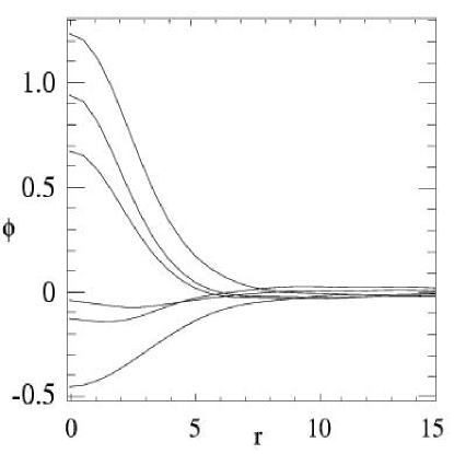
Figure 13: The profile of a localized oscillon at sequential time intervals, spanning half its oscillation period.

In order to strengthen our claim that oscillons are nucleated during the nonequilibrium evolution of $\phi({\bf x},t)$, the inset in figure 14 shows the distribution functions $f_{T}(R)$ and $f_{T}({\cal T})$ for the radii and period of oscillation, respectively. To make a comparison with deterministic oscillons, only fluctuations with $\phi_{\rm a}\geq 0.81$ (i.e. those that probe beyond the local maximum of the potential) and $\tau\geq 80$ are considered. That is, these are the lower bounds placed on the corresponding integrations over $F_{T}$. The bin widths are $\Delta R=\Delta{\cal T}=0.1$. The fitted curves are Gaussian functions with centers $R_{\rm ave}=4.3$ and ${\cal T}_{\rm ave}=8.5$ and widths $\sigma_{R}=0.4$ and $\sigma_{\cal T}=1.8$, respectively. To complete the comparison, consider a deterministic oscillon evolving in a time-independent effective potential that is representative of this case. From figure 9 a good approximation would be to take $\langle C(t)\rangle\simeq 0.4$, so that $\langle\delta\phi\rangle\simeq 0.15$. The effective mass can thus be obtained from the curvature of the left-hand well, given by eq. 16, and evaluates to $m_{\rm eff}=0.73$. Finally, from eq. 23, we find that the effective minimum radius for which the deterministic oscillon remains stable is $R_{\rm crit}^{\rm eff}=\sqrt{6}/m_{\rm eff}\simeq 3.37$. Comparing this result with figure 14 we see that, indeed, the emerging oscillons satisfy this requirement remarkably well. [Note that a proper comparison between oscillons that evolve in different potentials (i.e. for fields at different initial temperatures) always requires a suitable scaling of $\phi$, ${\bf x}$, and $t$.]

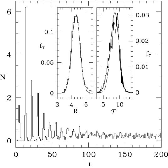
Figure 14: The number of oscillons nucleated as a function of time for $T=0.22$. Also shown (inset) are the probability distributions (solid lines) for the radius $R$ and period ${\cal T}$ of these oscillons. The fitted curves (dashed lines) are Gaussian functions.

Also shown in figure 14 is the distribution of nucleation times for the emerging oscillons. This quantity gives the number of oscillons nucleated between $t$ and $t+\Delta t$, with $\Delta t=1$. It is obtained by calculating the reduced distribution function $f_{T}(t_{\rm nuc})$ integrated over all the remaining variables. The same lower limits are used for the integrals over $\phi_{\rm a}$ and $\tau$, so that only long-lived large-amplitude fluctuations are considered. If there are $N_{\rm tot}$ such fluctuations, then the final expression for the number of oscillons nucleated as a function of time is

$$N(t)=N_{\rm tot}f_{T}(t_{\rm nuc}).$$ (27)

The sharp peaks in $N$ at early times, $t<60$, correspond to the synchronous emergence of oscillons. For $t>60$, this global ordering gives way to only local ordering, in which oscillons emerge at arbitrary times with similar probability. Even this local emergence disappears after approximately $t\geq 500$ (more on this later). Notice the correlation between the synchronous nucleation of oscillons and the energy loss from the zero-mode (c.f. figure 9) at early times, $t<60$. This phenomenon was observed for temperatures within $0.16\leq T\leq 0.26$ (see below). Below this temperature range the HHA is valid and no coherent structure emerges. Above this temperature range the field separates into large, slowly evolving thin-walled domains, signalling the approach to criticality.

IV.3 Synchronous emergence of order is due to parametric resonance

In order to understand the mechanism behind the observed synchronous emergence, we decompose the field as in eq. 14. The linearized equation satisfied by the Fourier modes of the fluctuations is

$$\ddot{\bar{\delta\phi}}=-\bar{\omega}^{2}(k)\bar{\delta\phi},$$ (28)

where

$$\bar{\omega}(k)^{2}=k^{2}+V_{\rm eff}^{\prime\prime}\left[\phi_{\rm ave}(t)\right].$$ (29)

In this approximation, the fluctuations obey a linear equation of motion with a time-dependent frequency determined by the value of $\phi_{\rm ave}(t)$. Equations of this type, generalized Mathieu equations, are known to exhibit parametric resonance, which can lead to exponential amplification ($\sim\exp{\eta t}$) in the oscillations of $\delta\phi(k,t)$ at certain wavelengths. They have been the focus of much recent attention in studies of reheating of the universe after an inflationary expansion phase kofman . To verify that this is the mechanism behind the synchronous amplification of oscillon modes early in the field’s evolution, we use in eq. 29 the anharmonic solution for $\phi_{\rm ave}(t)$ that would be obtained if the effective potential remained time-independent. That is, we require that $\phi_{\rm ave}(t)$ oscillates in the effective potential as determined immediately after the quench (i.e., without energy loss), just as the parametric driving force in generalized Mathieu equations oscillates with constant amplitude. In this sense, we are considering the initial response of the fluctuations to the oscillations of $\phi_{\rm ave}(t)$, without accounting for the subsequent transfer of energy between the two. Only with this approach can one achieve a constant exponential amplification of $\bar{\delta\phi}$ and thus a good measure of resonance. Even though this approximation only strictly holds for early times, the results obtained will confirm its validity in describing the essential physics behind the observed synchronous emergence.

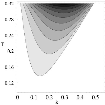
Figure 15: Lines of constant amplification rate for small-amplitude modes at various temperatures, beginning with $\eta_{\rm min}=2.8\times 10^{-2}$ for the bottom-most contour and increasing in increments of $\Delta\eta=1.3\times 10^{-2}$.

Figure 15 shows lines of constant exponential amplification rate $\eta$ of the fluctuations $\delta\phi(k,t)$ for various $k$ and $T$. At low temperatures, $T<0.14$, no modes are ever amplified. As the temperature is increased, so is the amplitude of oscillation in $\phi_{\rm ave}(t)$, gradually causing the band $0<k\leq 0.48$ to resonate. It is helpful at this point to consider what modes comprise a typical oscillon. To do so, we use a Gaussian ansatz for the oscillon with a fixed radius $R$, $\phi_{\rm osc}(r,t)\sim\exp(-r^{2}/R^{2})$ gleiser . The Fourier transform is itself a Gaussian with a characteristic radius $K=2/R$. Thus, a Gaussian in real space is generally comprised of the band $0\leq k\leq 2/R$ in $k$-space. Earlier [cf. figure 14] it was found that the average radius of the emergent oscillons is $R_{\rm ave}=4.3$ at an initial temperature $T=0.22$, which in this approximation corresponds to the band $0\leq k\leq 0.47$. This agrees very well with what is seen in figure 15. Although in this linear approximation the entire band does not resonate until higher temperatures, it is expected that in the full equation of motion the nonlinear coupling between modes will broaden the resonance band at lower temperatures.

We have observed that the synchronous emergence of oscillons occurs for initial temperatures $0.16\leq T\leq 0.26$. The lower bound is directly related to the nonlinear scattering between modes, which is absent at low temperatures. For temperatures above $T\simeq 0.26$, the appearance of large domains precludes the identification of oscillons. This is typical of the approach to criticality, where large spatial correlations in the field become more probable, destroying any local ordering. Thus, the observed quench-induced synchronous emergence of order is limited to temperatures sufficiently below $T_{c}$.

IV.4 Oscillons as bottlenecks for equipartition

In the introduction, we mentioned that long-lived locally-ordered structures may serve as bottlenecks to equipartition, as they slow down the distribution of energy between the system’s various degrees of freedom. Below, we present evidence that oscillons do precisely that. A more formal proof is left for future work.

A good observable to follow is the time evolution of $\langle\bar{\pi}^{2}(k,t)\rangle$ for different modes, which should become flat when thermal equilibrium is achieved and the equipartition theorem is satisfied. In highly dissipative systems (such as those governed by a Langevin equation of motion with a large viscosity coefficient), energy exchange between each mode and the thermal bath tends to dominate the dynamics. In the nonequilibrium closed system considered here, however, energy is only exchanged between the modes themselves, and the thermalization process turns out to be quite different.

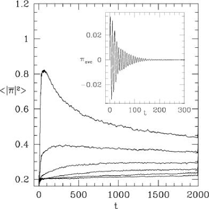
Figure 16: The time evolution of $\langle\bar{\pi}^{2}(k,t)\rangle$ for various modes (see text). The data is boxcar averaged over a window $\Delta t=10$. Also shown (inset) is the time evolution of $\pi_{\rm ave}(t)$, which attains equilibrium noticeably earlier than any of the higher modes shown.

In figure 16 we show the time evolution of $\langle\bar{\pi}^{2}(k,t)\rangle$ for the values $k$=0.25, 0.5, 0.75, 1.0, 1.25, and 1.5 (top to bottom lines, respectively). The curves are time-averaged over a window $\Delta t=10$ so that the large oscillatory behavior at early times ($t<60$) is suppressed. Also shown in the inset is the time evolution of $\pi_{\rm ave}(t)$, which exhibits the thermalization trend of the zero mode. $\pi_{\rm ave}(t)$ displays damped oscillatory motion before reaching its equilibrium value at $t\simeq 160$. This is roughly the time in which the mode $k=0.25$ reaches its maximum average kinetic energy. The mode $k=0.5$ also increases from $t=0$ to a maximum value at about the same time before decaying. For modes $k>0.5$, however, the general trend is to slowly absorb energy as they asymptotically approach their equilibrium values from below on time-scales that can be much longer than the lower-$k$ modes. There are two clear trends: small modes (with $k\leq 0.5$) grow very quickly and then relax to their final equilibrium values, while larger modes (with $k>0.5$) slowly approach theirs. Thus, it is reasonable to conclude that most of the zero-mode’s initial energy goes into its neighboring modes, those responsible for oscillon-like configurations [cf. figure 15], and only later on it is shared amongst larger $k$ modes. This seems to suggest that there is a two-step energy cascade, a fast one at early times to small-$k$ modes, followed by a slower one to larger $k$ modes. The early emergence of oscillons is consistent with this scenario.

We can further quantify this argument by introducing a measure of the entropy of the system based on the partitioning of the kinetic energy, $K({\bf k},t)=1/2|\bar{\pi}({\bf k},t)|^{2}$:

$$S(t)=-\int_{A}d\,^{2}k\,p({\bf k},t)\ln p({\bf k},t),$$ (30)

where

$$p({\bf k},t)=\frac{K({\bf k},t)}{\int d\,^{2}k\,K({\bf k},t)}$$ (31)

is the probability distribution of the kinetic energy in $k$-space. $S(t)$ attains its maximum value when equipartition is satisfied, and $p({\bf k},t)=A^{-1}$ where $A$ is the area of this space. This occurs both at the initial thermalization $(t=0)$ and final equilibrium states, since in these cases all modes carry the same fractional kinetic energy. At these times we recover the thermodynamic entropy of the system, $S_{\rm eq}=\ln A$, which is a measure of the number of accessible states in the system. [The numerical implementation gives $S_{\rm eq}=\ln N$, where $N$ is the number of lattice points, or degrees of freedom.] In figure 17 we show the change of $S(t)$ from the initial state, $S(t=0)-S(t)$, for the system at $T=0.22$. At late times ($t>100$), we have found that the system equilibrates exponentially in a time-scale $\tau\simeq 500$. At early times, the localization of energy at lower $k$ modes, corresponding to the synchronous emergence of oscillons, prolongs this approach to equipartition. The inset of figure 17 shows the large oscillations in the early evolution of $S(t)$ (dotted line). Also shown (solid line) is the average between successive peaks of $S(t)$, with a plateau at $30\leq t\leq 100$ that coincides with the maximum oscillon presence in the system. This is to be contrasted with an exponential approach to equilibrium. Thus, we see evidence that oscillon configurations indeed serve as early bottlenecks to equipartition, temporarily suppressing the cascading of energy from low-$k$ modes to higher modes.

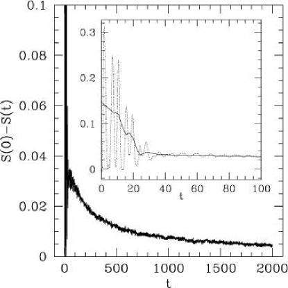
Figure 17: The change of $S(t)$ from the initial state for closed systems at $T=0.22$. The exponential approach to equilibrium is clear at late times. The inset illustrates the role of oscillons as a bottleneck to equipartition.

V Resonant Nucleation

We will now investigate the dynamics with the ADW potential, that is, for values of $\alpha>3/2$. Homogeneous nucleation predicts that, had the system been prepared in the metastable state at $\phi=0$ at some temperature $T$, its decay rate per unit area would be controlled by the Arrhenius factor, $\Gamma_{\rm HN}\sim\exp[-E_{b}/T]$, where $E_{b}$ is the free-energy barrier for the nucleation of a critical nucleus or bounce langer ; domb . (We set $k_{B}=1$.) It is often overlooked that this result is quite sensitive to how the initial state is prepared. It assumes that the bounce is nucleated within a homogeneous background, by adopting a perturbative Gaussian approximation for the evaluation of the partition function. In other words, it assumes that no large-amplitude perturbations are present in the system gleiser-heckler ; tetradis . It is also well-known that there are discrepancies between the theoretical prediction from homogeneous nucleation and a large array of experimental results concerning nucleation rates, from He³ leggett and nematic liquid crystals degennes to martensitic materials and polycrystals offerman to fluids bartell and numerical simulations gleiser_nuc . More often than not, theoretical estimates greatly underestimate nucleation rates. Surely, many of these discrepancies are related to limited knowledge of the nonequilibrium processes leading to nucleation at the atomic or mesoscopic scale for various materials. However, we propose here that in certain cases the problem is rooted on the detailed set up of the initial metastable state. In particular, the quench we propose in this work, which may be mimicked in experimental situations, generates an instability capable of greatly accelerating the decay of the metastable state. In fact, we have observe that, for a range of temperatures, the nucleation rate per unit area is not that of homogeneous nucleation, $\Gamma_{\rm HN}=C\exp[-E_{b}/T]$, but a power law, $\Gamma_{\rm RN}=C(E_{b}/T)^{-B}$, where $E_{b}(\alpha)$ is the critical nucleus free energy and the exponent $B$ is weakly temperature-dependent. RN stands for Resonant Nucleation. The power law applies precisely within the temperature range where we observe the synchronous emergence of oscillons at early times, $0.18\leq T\leq 0.24$, as we show next.

The change in $\alpha$ will not modify the basic parametric amplification mechanism discussed above in the context of the SDW: for a range of temperatures, oscillons are still nucleated in synchrony at early times. The difference is that, for $\alpha>\alpha_{c}$, the system must reach the global free-energy minimum at $\phi_{+}(\alpha)$. [Of course, for large enough temperatures, $T>0.26$, and/or small energy barriers the system will go straight into the global minimum, a cross-over decay. We are not interested in these cases.]

In the usual treatment, the critical nucleation is described as the saddle-point in field-configuration space, the unstable direction dictated by the negative eigenvalue associated with the growth of the critical nucleus. This is given by the solution of the equation $\phi^{\prime\prime}+(1/r)\phi^{\prime}=V^{\prime}$, with appropriate boundary conditions, which determines the 2d bounce langer . In the absence of forcing, which is the case for homogeneous nucleation, the system will randomly probe phase space until it eventually “finds” the saddle point. The presence of quench-induced large-amplitude fluctuations in the field will drastically accelerate its decay. In figure 18 we show the evolution of the order parameter $\phi_{\rm ave}(t)$ as a function of time for several values of asymmetry, $1.518\leq\alpha\leq 1.56$ for $T=0.22$. Not surprisingly, as $\alpha\rightarrow\alpha_{c}=1.5$, the field remains longer in the metastable state, since the nucleation energy barrier $E_{b}\rightarrow\infty$ at $\alpha_{c}$. However, a quick glance at the time axis shows the fast decay time-scale, of order $10^{1-2}$. For comparison, for $1.52\leq\alpha\leq 1.56$, homogeneous nucleation would predict nucleation time-scales of order $\sim 10^{56}\leq\tau_{\rm HN}\leq 10^{21}$ (in dimensionless units), respectively. [The nucleation barriers are, $E_{b}(\alpha=1.158)=33.67$ and $E_{b}(\alpha=1.56)=13.10$.] Clearly, while for smaller asymmetries $\phi_{\rm ave}(t)$ displays similar oscillatory behavior to the SDW case before transitioning to the global minimum, as $\alpha$ is increased (asymmetry in potential is increased) the number of oscillations decreases sharply.

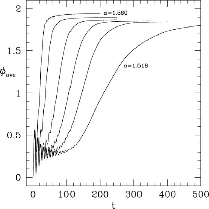
Figure 18: The evolution of the order parameter $\phi_{\rm ave}(t)$ at $T=0.22$ for several values of the asymmetry. (From left to right, $\alpha=1.56,1.542,1.53,1.524,1.521,1.518$.) Each curve is an ensemble average over 100 runs.

In figure 19 we show the log-log plot of the ensemble-averaged nucleation time-scales as a function of the nucleation barrier, or critical droplet free energy, $E_{b}/T$ for different temperatures, $T=0.18,0.20,$ and $0.22$. The error bars are computed from the dispersion of the measured time scales within the ensemble. The best fit is a power law, $\tau_{RN}\propto(E_{b}/T)^{B}$, with $B=2.440\pm 0.008$ for $T=0.20$ and $T=0.22$, and $B=3.36\pm 0.04$ for $T=0.18$. This simple power law holds for the same range of temperatures where we have observed the synchronous emergence of oscillons. [The range is similar for both SDW and ADW.] It is not surprising that the exponent $B$ is larger for $T=0.18$, where the synchronous emergence of oscillons is marginal: at lower temperatures, the oscillations of the field’s zero mode have lower amplitude and oscillons become rarer. In fact, as we remarked before, we have not observed any for $T<0.16$ for the SDW. For lower temperatures, we should thus expect a smooth transition into the exponential time-scales of homogeneous nucleation. We intend to analyse this transition and to obtain an analytical explanation for the power law in a forthcoming publication. As a first step in this direction, we present below what we believe is the mechanism by which the transition completes for different nucleation barriers.

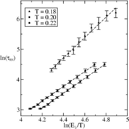
Figure 19: The decay time-scale $\tau_{\rm RN}$ for resonant nucleation as a function of critical nucleation free-energy barrier $E_{b}/T$ at $T=0.18$, $0.2$, and $0.22$. The best fit is a power-law with exponent $B\simeq 2.44$ for $T=0.20$ and $0.22$ and $B=3.36$ for $T=0.18$.

First, note that the error bars in figure 19 increase with nucleation barrier. This spread in time scales is related to the dynamics of the system. For $\alpha\rightarrow\alpha_{c}$ the radius of the nucleation bubble diverges, $R_{b}\rightarrow\infty$. Clearly, due to the disparity between the power law and the exponential time scales, the mechanism by which the system approaches the global minimum is not through a random search in configuration space as is the case for homogeneous nucleation. Instead, we argue that oscillons will act as seeds for the nucleation of a critical fluctuation. The way in which this happens depends on the nucleation barrier. If $\alpha\gtrsim\alpha_{c}$, the critical nucleus will have a radius much larger than a typical oscillon [cf. figure 14]; it will appear as two or more oscillons coalesce. As $\alpha$ is increased further, the radius of the critical nucleus decreases, approaching that of an oscillon. In this case, a single oscillon may become the critical nucleus and promote the decay of the metastable state. This explains the small number of oscillations on $\phi_{\rm ave}(t)$ as $\alpha$ is increased [cf. figure 18]. To corroborate our argument, in figure 20 we contrast the critical nucleation radius with that of oscillons for different values of energy barrier at $T=0.22$. The average oscillon radius [cf. figure 14] is $R_{\rm ave}=4.30\pm 0.4$, and is identified by the dashed line, with the dotted lines denoting its dispersion. The critical nucleus radius, $R_{b}$, is equal to $R_{\rm ave}$ for $\alpha\simeq 1.575\pm 0.0075$, or $E_{b}/T=53.9\pm 0.4$. Thus, for $\alpha\gtrsim 1.568$ one cannot distinguish between a single oscillon and a critical bubble. Since, as we have seen, oscillons appear very early on, the decay happens quite fast. For $1.5<\alpha<1.568$, approximately, the critical nucleus is the result of the coalescence of two or more oscillons. They diffuse through the lattice and scatter, forming bound states, somewhat as in kink-antikink breathers in 1d field theory campbell ; hanggi . We emphasize that these values are only approximate; they do not include the increase in coalescence rates due to diffusive motions on the lattice or an enhancement on the unstable growth of oscillons due to perturbations. We expect that the one-oscillon decay will ensue for smaller values of $\alpha$. In website the reader can see a few representative simulations.

Clearly, these arguments can be refined. In particular, the details of oscillon coalescence remain unexplored. However, they encapsulate the basic mechanism by which metastable states decay via resonant nucleation, as seen in numerical simulations.

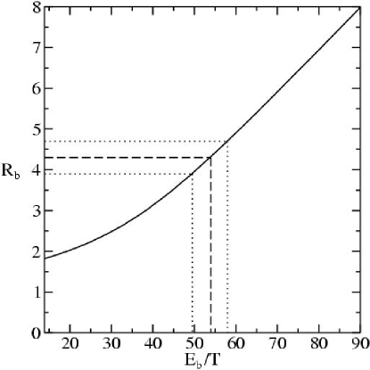
Figure 20: The critical nucleus radius as a function of its energy barrier at $T=0.22$. The dashed line shows the average radius for nucleated oscillons, while the dotted lines denote the dispersion of its value.

VI Summary and Outlook

We have investigated the nonequilibrium dynamics of a double-well model with a 2d scalar order parameter. The system was initially prepared in thermal equilibrium at a fixed temperature in a anharmonic single-well potential, $V(\phi)=\frac{1}{2}\phi^{2}+\frac{1}{8}\phi^{4}.$ We then turned on a cubic interaction with tunable strength so that the resulting double-well potential can be symmetric (SDW) or asymmetric (ADW). The turning-on of the interaction can be interpreted as a “quench,” as it occurs within a time-scale faster than any in the system. The system is thus tossed into a double-well potential and, through its nonlinear interactions, redistributes its energy until it reaches equipartition. For the SDW case, we have observed that this approach to equilibrium occurs as a two-step energy cascade: quickly at first, as the zero-mode relinquishes its energy to nearby (in $k$-space) long-wavelength modes, and slower later, as the energy is partitioned with the short-wavelength modes. Although we have adopted the language of nonequilibrium field theory, we remark that one could equally well treat the system as a microcanonical ensemble with fixed energy $E$.

We showed that, for a range of initial temperatures, the initial stages of the dynamics are dominated by damped oscillations of the field’s zero mode, which, via parametric resonance, excite the modes associated with coherent structures named oscillons. We also showed that the initial emergence of oscillons occurs at the breakdown of the homogeneous Hartree approximation. Furthermore, this emergence occurs in synchrony, characterizing a global emergence phenomenon. As oscillons are long-lived coherent structures, they act as bottlenecks for equipartition. The observed synchronous emergence dies away with the damping of the zero-mode oscillations. Oscillons then appear randomly throughout the lattice, until such a time when there isn’t enough energy in long-wavelength modes.

We then investigated the dynamics in ADWs, where the final equilibrium state is at the global minimum of the potential. The system was thermalized as for the SDW, in its metastable well. Also as before, the quenching induces damped oscillations of the field’s zero mode and oscillons emerge. We observed that, approximately for the same range of temperatures where oscillons emerged in the SDW case, the decay rate was greatly enhanced, when compared to homogeneous nucleation results. In fact, we obtained an excellent fit to a power law decay time scale, $\tau_{\rm RN}\propto[E_{b}/T]^{B}$, where $E_{b}$ is the energy of the critical nucleus or bounce and $B$ is a numerical exponent, $2.44\leq B\leq 3.36$, for the temperatures we investigated. We argued that there were two main mechanisms for what we called resonant nucleation: for small asymmetries, the critical nucleus appears as two or more oscillons coalesce. For larger asymmetries, a single oscillon grows to become the critical nucleus, promoting the decay of the metastable state.

The greatly accelerated decay is due to the resonant oscillations of the zero mode, induced by the quenching. It is thus plausible that such behavior may be observed in several related systems with a scalar order parameter. The emergence of oscillons in granular materials appears due to the sinusoidal vibrations of their container umbanhowar ; this is mimicked here by the oscillation of the field’s zero mode, which corresponds to the periodic oscillation of the whole lattice. As for granular materials, patterns emerge above a certain amplitude. We do not claim to have modelled the behavior of granular materials here, but believe to have captured some of the essential physics. Also, since the model here falls in the Ising universality class, we expect that similar qualitative behavior should occur, for example, in ferromagnets and possibly binary liquids and metal alloys, if long wavelength oscillations can be induced by the quenching process.

- (1) D. Walgraef, Spatio-temporal Pattern Formation (Springer, New York, 1997); A. I. Olemskoi and V. F. Klepikov, Phys. Rep. 338, 571 (2000).
- (2) Y. Bar-Yam, Dynamics of Complex Systems (Addison-Wesley, Reading, MA, 1997).
- (3) M. C. Cross and P. C. Hohenberg, Rev. Mod. Phys. 65, 851 (1993); Y. Kuramoto, Chemical Oscillations, Waves, and Turbulence (Springer, Berlin, 1984).
- (4) N. Goldenfeld, Lectures on Phase Transitions and The Renormalization Group, Frontiers in Physics, V. 85 (Addison-Wesley, NY, 1992).
- (5) A. Aharoni, Introduction to the Physics of Ferromagnetism (Oxford University Press, NY, 1996).
- (6) P. G. de Gennes, The Physics of Liquid Crystals (Oxford University Press, Oxford, 1993).
- (7) N. M. Shnerb, Y. Louzoun, E. Bettelheim, and S. Solomon, S., PNAS, 97, 10322-10324 (2000).
- (8) J. Ford, Phys. Rep. 213, 271 (1992).
- (9) S. Flach and C. R. Willis, Phys. Rep. 295, 181 (1998)
- (10) R. Reigada, A. Sarmiento, and K. Lindenberg, cond-mat/0210326
- (11) R. Rajamaran, Solitons and Instantons (North-Holland, Amsterdam, 1987); T. D. Lee and Y. Pang, Phys. Rep. 221, 251 (1992).
- (12) A. Vilenkin and E. P. S. Shellard, Cosmic Strings and Other Topological Defects (Cambridge University Press, Cambridge, 1994).
- (13) S. Coleman, Aspects of Symmetry, Cambridge University Press (Cambridge, UK 1985)
- (14) D. K. Campbell, J. F. Schonfeld, and C. A. Wingate, Physica 9D, 1 (1983).
- (15) For an exception see, S. Digal, R. Ray, S. Sengupta, and A. M. Srivastava, Phys. Rev. Lett. 84, 826 (2000).
- (16) M. Gleiser and R. Howell, arXiv:cond-mat/0209176, in press Phys. Rev. E (RC).
- (17) M. Gleiser, Phys. Rev. D 49, 2978 (1994); E. J. Copeland, M. Gleiser, and H. R. Muller, Phys. Rev. D 52, 1920 (1995); E. B. Bogomol’nyi, Sov. J. Nucl. Phys. 24, 449 (1976).
- (18) D. Bettison and G. Rowlands, Phys. Rev. E 55, 5427 (1997); C. Crawford and H. Riecke, Phys. Rev. E 65, 066307 (2002).
- (19) P. Umbanhowar, F. Melo, and H. Swinney, Nature 382, 793 (1996); L. S. Tsimring and I. S. Aranson, Phys. Rev. Lett. 79, 213 (1997); S.-O. Jeong and H.-T. Moon, Phys. Rev. E 59, 850 (1999).
- (20) O. M. Umurhan, L. Tao, and E. A. Spiegel, Ann. N. Y. Acad. Sci. 867, 298 (1998).
- (21) J. S. Langer, in Solids Far from Equilibrium, Ed. C. Godrèche (Cambridge University Press, Cambridge, 1992).
- (22) J. D. Gunton, M. San Miguel, and P. S. Sahni, in Phase Transitions and Critical Phenomena, Ed. C. Domb and J. L. Lebowitz, v. 8 (Academic Press, London, 1983); J. D. Gunton, J. Stat. Phys. 95, 903 (1999).
- (23) M. Gleiser, R. C. Howell, and R. O. Ramos, Phys. Rev. E 63, 036113 (2002).
- (24) M. A. Muñoz and R. Pastor-Satorras, Phys. Rev. Lett. 90, 204101 (2003).
- (25) D. Chandler, Introduction to Modern Statistical Mechanics, (Oxford University Press, Oxford, 1987).
- (26) G. Aarts, G. F. Bonini, and C. Wetterich, Phys. Rev. D 63, 025012 (2000); G. Aarts, G. F. Bonini, and C. Wetterich, Nucl. Phys. B 587, 403 (2000).
- (27) D. Boyanovsky, C. Destri, and H. J. de Vega, arXiv:hep-ph/0306124.
- (28) J. Borrill and M. Gleiser, Nucl. Phys. B 483, 416 (1997).
- (29) M. Gleiser, Phys. Rev. Lett. 73, 3495 (1994); J. Borrill and M. Gleiser, Phys. Rev. D51, 4111 (1995).
- (30) see http://www.dartmouth.edu/cosmos/oscillons
- (31) W. Press, S. Teukolsky, W. Vetterling, and B. Flannery, Numerical Recipes in C, (Cambridge University Press, Cambridge UK, 1992).
- (32) M. Gleiser and A. Sornborger, Phys. Rev. E 62, 1368 (2000);A. Adib, M. Gleiser, and C. Almeida, Phys. Rev. D 66, 085011 (2002).
- (33) Here is an incomplete list of references: G. N. Felder and L. Kofman, Phys. Rev. D 63, 103503 (2001); P. B. Greene and L. Kofman, Phys. Lett. B 448, 6 (1999); P. B. Greene, L. Kofman, A. D. Linde and A. A. Starobinsky, Phys. Rev. D 56, 6175 (1997); D. Boyanovsky, H. J. de Vega and R. Holman, arXiv:hep-ph/9701304; D. Boyanovsky, M. D’Attanasio, H. J.de Vega, R. Holman and D. S. Lee, Phys. Rev. D 52, 6805 (1995); D. Boyanovsky, H. J. de Vega and R. Holman, arXiv:hep-ph/9903534.
- (34) M. Gleiser and A. Heckler, Phys. Rev. Lett. 76, 180 (1996).
- (35) A. Strumia, N. Tetradis and C. Wetterich, Phys. Lett. B 467, 279 (1999).
- (36) A. J. Leggett and S. K. Yip, in Helium Three, edited by W. P. Halperin and L. P. Pitaevskii (North-Holland, Amsterdam, 1990).
- (37) S. E. Offerman et al., Science 298 (2002) 1003.
- (38) J. Huang and L. S. Bartell, J. Phys. Chem. 99, 3924 (1994).
- (39) M. Alford and M. Gleiser, Phys. Rev. D48, 2838 (1993); G. T. Valls and G. F. Mazenko, Phys. Rev. B 42, 6614 (1990); K. Park, P. A. Rikvold, G. M. Buendia, M.A. Novotny, arXiv:cond-mat/0307595.
- (40) P. Hänggi, F. Marchesoni, and P. Sodano, Phys. Rev. Lett. 60, 2563 (1988).