Solvation force for long ranged wall-fluid potentials

Abstract

The solvation force of a simple fluid confined between identical planar walls is studied in two model systems with short ranged fluid-fluid interactions and long ranged wall-fluid potentials decaying as $-Az^{-p},z\to\infty$, for various values of $p$. Results for the Ising spins system are obtained in two dimensions at vanishing bulk magnetic field $h=0$ by means of the density-matrix renormalization-group method; results for the truncated Lennard-Jones (LJ) fluid are obtained within the nonlocal density functional theory. At low temperatures the solvation force $f_{solv}$ for the Ising film is repulsive and decays for large wall separations $L$ in the same fashion as the boundary field $f_{solv}\sim L^{-p}$, whereas for temperatures larger than the bulk critical temperature $f_{solv}$ is attractive and the asymptotic decay is $f_{solv}\sim L^{-(p+1)}$. For the LJ fluid system $f_{solv}$ is always repulsive away from the critical region and decays for large $L$ with the the same power law as the wall-fluid potential. We discuss the influence of the critical Casimir effect and of capillary condensation on the behaviour of the solvation force.

I Introduction

Fluid mediated interactions between two surfaces or large particles, usually referred to as solvation forces $f_{solv}$ evans:90:0 , may lead to subtle effects  israelachvili:91:0 that can be relevant in colloidal systems and for many applications and modern technologies such as lubrication, adhesion or friction. There is a rapidly growing literature on experimental investigations and other phenomena associated with solvation forces. Direct measurements with the Surface Force Apparatus (SFA) israelachvili:78:0 have revealed the richness of behaviour of these forces, for example, their sensitivity to specific properties of the intervening fluid. Dependence of the solvation force on the chemical and physical properties of confining surfaces is also of much interest. Different surfaces have been developed and used in SFA by adsorbing or depositing a thin film of some other material on a mica surface, for example, lipid monolayers or bilayers, metal films, polymer films or other macromolecules such as proteins israelachvili:91:0 ; smith:88:0 ; parker:88:0 ; lee:89:0 .

On the other hand, the theory of the solvation forces which would help to interpret measurements performed for different liquids and different surfaces is far from being complete even for simple model systems. One of the issues which has not been systematically investigated is how the properties of the solvation force $f_{solv}(L)$, such as its sign, magnitude and asymptotic dependence on the distance between surfaces, vary with the range and the strength of the substrate-fluid potential and with the thermodynamic state. In the present paper we address these issues for a simple fluid confined between two identical parallel solid substrates separated by a distance $L$.

The majority of results available for the solvation force in this simple system comes from a model fluid in which both the fluid-fluid interatomic potential and the wall-fluid potential $V_{s}({\bf r})$ are of short range. Here, by $f_{solv}(L)$ we are referring only to the fluid contribution to the force, the direct wall-wall contribution is not included. Let us summarize briefly results that are the most relevant for the present paper. The precise form of the solvation force depends on the details of $V_{s}({\bf r})$, the bulk state point, as well as on $L$. Theory and computer simulations show that at small wall separations the solvation force exhibits oscillatory behaviour with $L$. These oscillations, observed in direct measurements of the solvation force in real fluids, reflect packing effects that produce oscillations in the density profile for liquids near walls  evans:90:1 . The behaviour of $f_{solv}(L)$ reflects the behaviour of the density profile also in the limit of large separation, $L\to\infty$. General statistical mechanical arguments predict that far from the bulk critical temperature $T_{c}$ and from any phase transitions (condensation phenomena) $f_{solv}(L)$ for $L\to\infty$ must decay to zero in the same fashion as the profile at a single wall decays to its bulk value, i.e., as the radial distribution function $g(r)$ of the bulk fluid evans:92:0 ; henderson:92:0 ; evans:93:0 ; evans:94:1 . Thus, for $V_{s}({\bf r})$ of finite range and $L\to\infty$, $f_{solv}(L)\sim e^{-\alpha_{0}L}$ or, for sufficiently high densities and/or temperatures, (states on the oscillatory side of the so-called Fisher-Widom line) $f_{solv}(L)\sim exp(-\alpha_{0}L)\cos(\alpha_{1}L)$. The quantities $\alpha_{0}$ and $\alpha_{1}$ depend on only the bulk pair correlation function. The sign of the solvation force and its temperature dependence at fixed $L$ are available from mean-field (lattice, Landau, density functional) analyses evans:86:0 ; marconi:88:0 ; parry:92:0 ; krech:97:0 ; dietrich:98:0 ; upton:99:0 and from exact transfer matrix methods for two-dimensional strips evans:94:0 . For simple fluids confined between identical walls $f_{solv}(L)<0$ for large $L$, i.e., the net force between the substrates is attractive for large separations. Away from the bulk critical temperature $T_{c}$, $f_{solv}(T)$ is small in magnitude (weakly attractive). On approaching $T_{c}$ at vanishing ordering field, $h=0$, where $h\sim\mu-\mu_{sat}$, where $\mu_{sat}$ is the chemical potential at coexistence, the force increases in magnitude and exhibits a minimum. For strongly adsorbing walls this minimum is located above $T_{c}$ and occurs for $L$ of the order of the bulk correlation length $\xi_{b}$. Critical scaling arguments predict fdg:78:0 ; fss that at bulk criticality $f_{solv}(L)$ decays algebraically for large separations, i.e.,

$$f_{solv}(L)\sim k_{B}T_{c}A_{12}(d-1)L^{-d}~{}~{}~{}~{}~{}~{}~{}~{}~{}~{}~{}~{}~{}L\to\infty.$$ (1)

$d$ is the spatial dimension and $A_{12}$ a universal number (Casimir amplitude) for $2\leq d\leq d_{>}$, where the upper critical dimension $d_{>}=4$ for the Ising universality class. $A_{12}$ is negative for identical walls, i.e. the Casimir force is attractive.

In the present paper we study two model systems in which fluid-fluid interactions are short ranged but the substrate-fluid potential $V_{s}({\bf r})$ is long ranged, and enquire how the features of the solvation force described above change with the range and the strength of $V_{s}({\bf r})$. As a first system we consider a (Ising) lattice gas in a slit geometry subject to identical boundary fields which depend on the distance $l$ of a lattice site from the boundary

$$V_{s}({\bf r})\equiv H^{s}_{l}=\frac{h_{1}}{l^{p}}$$ (2)

with $h_{1},p\geq 0$. The Ising model is particularly useful in fundamental studies of finite-size and surface effects in confined fluids since exact calculations are available, at least in two dimensions and for short ranged boundary fields evans:94:0 ; au-yang:75:0 ; abraham:71:0 ; abraham:73:0 ; maciolek:96:0 ; maciolek:99:0 . Another advantage is that in $d=2$ this model is amenable to the systematic investigation for arbitrary boundary and bulk fields by means of density-matrix renormalization-group (DMRG) method clsys . The DMRG method, based on the transfer matrix approach, provides a very efficient algorithm for constructing the effective transfer matrices for large systems. Comparisons with exact results for the case of vanishing bulk magnetic field and boundary fields acting only on spins in the surface layers show that this technique gives very accurate results in a wide range of temperatures, including near the bulk critical temperature, and for large widths of the strip maciolek:99:0 ; carlon:98:0 ; drzew:00:1 . Here, using the DMRG method we calculate $f_{solv}$ as a function of temperature along the bulk two-phase coexistence line, i.e., for vanishing bulk magnetic field, for different values of $p$, $h_{1}$ and $L$. We also study the asymptotic decay, with $L$, of the solvation force for strongly adsorbing walls (large $h_{1}$) and temperatures away from $T_{c}$.

Lattice models of a confined fluid cannot describe packing effects that are reflected in the oscillations of the solvation force at small wall separations. The other failing of the (Ising) lattice gas model is that it has an exact particle-hole symmetry. For real fluids such symmetry is only approximate which can be of relevance for the properties of $f_{solv}$ away from criticality. Therefore, to make our analysis more complete we also study a Lennard-Jones (LJ) fluid in a slit geometry. Specifically, we consider a truncated LJ 12-6 fluid-fluid intermolecular pair potential and a wall-fluid potential of the form:

$$V_{s}({\bf r})\equiv V_{s}(z)=4\varepsilon_{fw}\left[\frac{2}{15}\left(\frac{\sigma}{z}\right)^{9}-\left(\frac{\sigma}{z}\right)^{p}\right]\;,$$ (3)

where $p=2,3$; $\sigma$ is the diameter of the fluid species, while $\varepsilon_{fw}$ describes the strength of the wall–fluid interactions. We note that for $p=3$, $~{}V_{s}(z)$ models a wall which is assumed to comprise a half space of LJ particles israelachvili:91:0 . We calculate $f_{solv}$ using a nonlocal density functional theory (DFT) along a similar thermodynamic path as in the Ising system, i.e., as a function of the temperature along the bulk two phase-coexistence line and at the critical density for $T>T_{c}$. Our results refer to the densities on the liquid side of this line. We also investigate the asymptotic dependence of the solvation force on the distance between the walls at fixed temperature away from $T_{c}$.

The asymptotic behaviour of the solvation force for the Lennard-Jones fluid follows from the analysis by Attard et al. attard:91:0 based on the wall-particle Ornstein-Zernike (OZ) equations. Using the hypernetted-chain closure these authors derived the interaction free energy per unit area between the planar walls $F_{00}(L)$ as a convolution of wall-solvent pair-correlation functions. For a power-law fluid-fluid interaction potential $-Ar^{-n},n>3,r\to\infty$ and a wall-fluid potential decaying as $-Bz^{-p}$ for $z\to\infty$ a formula for the asymptotic behaviour of $F_{00}(L)$ (Eq.(6.11) of Ref.attard:91:0 ) is

$$F_{00}(L)\sim\beta u_{00}(L)+\frac{2\rho B}{p-1}L^{1-p}-\frac{2\pi\rho^{2}A}{(n-2)(n-3)(n-4)}L^{4-n},~{}~{}~{}~{}~{}L\to\infty$$ (4)

where $u_{00}(L)$ is the direct wall-wall interaction potential per unit area and $\rho$ is the density of the fluid. From Eq. (4) it follows that in the case of truncated LJ fluid, when the power-law tails are omitted, the behaviour of $f_{solv}(L)=-\left(\partial F_{00}(L)/\partial L\right)_{T,\mu}$ for large $L$ is

$$f_{solv}(L)\sim\frac{2\rho B}{L^{p}},~{}~{}~{}~{}~{}~{}~{}~{}~{}~{}~{}~{}L\to\infty,$$ (5)

where $B=4\varepsilon_{fw}$ and we have neglected the contribution due to the direct wall-wall interaction potential. Thus the solvation force is repulsive and decays with the same power law as the wall-fluid potential. The above prediction is treated as a reference point for the analysis of the asymptotic behaviour of our results. We find that, as one expects, Eq. (5) is indeed valid provided one is away from the critical temperature and from any phase transitions. The influence of the critical Casimir effect and of capillary condensation on the behaviour of the solvation force is also discussed in the present paper.

It is reasonable to expect that away from $T_{c}$ and from any phase transitions the ’magnetic’ analog of the solvation force in system of Ising spins subject to identical boundary fields should have the same asymptotic decay power law as the boundary field $H^{s}_{l}$. Somewhat surprisingly, this is not the case for temperatures far above $T_{c}$ where we find that $f_{solv}(L)$ decays as $L^{-(p+1)}$ for $L\to\infty$. For low temperatures the decay agrees with the prediction (5). In order to understand the nature of this particular behaviour we analyse the appropriate Landau theory.

The paper is organized as follows. Section II is devoted to the Ising model studies. We define the model and briefly review the known results pertinent to the present studies. We then proceed to describe the results of the DMRG studies. In Sec. III a continuum Landau theory is investigated for long ranged surface fields. In Sec. IV DFT calculations are presented and discussed. Section  V summarizes our results and makes some conclusions.

II Ising model results

II.1 The model

We consider an Ising ferromagnet in a slit geometry subject to identical boundary fields. Our DMRG results refer to the $d=2$ strip defined on the square lattice of the size $L\times M,M\to\infty$. The lattice consists of $L$ parallel rows at spacing $a=1$, so that the width of the strip is $La=L$. We label successive rows by the index $l$. At each site, labeled $(l,k)$, there is an Ising spin variable taking the value $\sigma_{lk}=\pm 1$. We assume nearest-neighbour interactions of strength $J$ and Hamiltonian of the form

$${\cal H}=-J\{\sum_{<lk,l^{\prime}k^{\prime}>}\sigma_{lk}\sigma_{l^{\prime}k^{\prime}}+\sum_{l=1}^{L}H_{l}\sum_{k}\sigma_{lk}\}.$$ (6)

The first term in (6) is a sum over all nearest-neighbor pairs of sites while in the second term $H_{l}=H^{s}_{l}+H^{s}_{L+1-l}$ is the total boundary magnetic field experienced by a spin in row $l$. The single-boundary field $H^{s}_{l}$ is assumed to have a form:

$$H^{s}_{l}=\frac{h_{1}}{l^{p}}$$ (7)

with $p>0$, and the reduced amplitude of the boundary field $h_{1}\geq 0$.

II.2 Solvation force for short ranged boundary fields

All previous work on the behaviour of the solvation force in Ising films used localized boundary fields acting only on spins in surface layers $l=1$ and $l=L$:

$$H_{l}=h_{1}\delta_{1,l}+h_{2}\delta_{L,l}.$$ (8)

In the limit $h_{1},h_{2}\to\infty$ Eq. (8) corresponds to the $(++)$ fixed spin boundary conditions, widely studied in the literature.

The total excess free energy per unit area for the case of identical surface fields $h_{1}=h_{2}$ and vanishing bulk magnetic field $h=0$ can be written as

$$f_{ex}(L)\equiv L(f(L,T,h_{1})-f_{b}(T))+2f_{w}(T,h_{1})+f^{*}(L,T,h_{1})$$ (9)

where $f$ is the total free energy per site, $f_{b}$ is the bulk free energy, $f_{w}$ is the $L$-independent surface excess free energy contribution from each surface, and $f^{*}$ is the finite-size contribution to the free energy. All energies are measured in units of $J$ and the temperature in units of $J/k_{B}$. $f^{*}$, which vanishes for $L\to\infty$, gives rise to the generalized force, which is analogous to the solvation force between the walls in the case of confined fluids evans:90:0 ,

$$f_{solv}=-(\partial f_{ex}(L)/\partial L)_{T,h_{1}}.$$ (10)

For identical surface fields the solvation force is attractive for all thermodynamic states, i.e., $f_{solv}<0$. The asymptotic decay of the solvation force depends on the temperature range. For temperatures sufficiently far away from the bulk critical temperature $T_{c}$, $f_{solv}$ decays as $\exp(-L/\xi_{b})$, where $\xi_{b}$ is the bulk correlation length evans:94:0 . Near $T_{c}$, $f_{solv}$ becomes long ranged as a result of critical fluctuations  fdg:78:0 , a phenomenon which is known as the critical Casimir effect krech:99:0 . At $T=T_{c}$ and $h=0$ the asymptotic decay is given by Eq. (1). For the case of $(++)$ boundary conditions the temperature dependence of the solvation force at fixed $L$ and $h=0$, or equivalently the scaling function $W_{++}({\tilde{y}})$ is defined by

$$f_{solv}/k_{B}T_{c}\equiv(d-1)L^{-d}W_{++}({\tilde{y}}),$$ (11)

where the scaling variable ${\tilde{y}}\equiv\tau(L/\xi_{0})^{1/\nu}$. In $d=2$ the scaling function was determined by exact transfer matrix methods evans:94:0 . Here $\tau\equiv(T-T_{c})/T_{c}$ and $\xi=\xi_{0}\tau^{-\nu}$ (with $\nu=1$ in $d=2$) is the bulk correlation length. It was found that $f_{solv}$ plotted as a function of temperature attains a pronounced minimum above the bulk critical temperature $T_{c}$ when ${\tilde{y}}\equiv\tau(L/\xi^{+}_{0})^{1/\nu}=2.23$, or $L\sim 2.23\xi$. The amplitude of the correlation length above $T_{c}$ is $\xi^{+}_{0}\approx 0.5673$.

It was also shown evans:94:0 that the scaling function has the property, for $d=2$,

$$W_{++}({\tilde{y}})=W_{00}(-{\tilde{y}}),$$ (12)

where subscript $00$ refers to $h_{1}=h_{2}=0$. This implies that at $h=0$ and fixed $L$ the function $f_{solv}(T)$ evaluated for free boundaries has its minimum below $T_{c}$. The behaviour of the function $f_{solv}(T)$ in the crossover between $h_{1}=\infty$ and $h_{1}=0$ has not been studied. In the next section we perform such an investigation for both short ranged and long ranged boundary fields.

Finally, we note that for free boundaries $h_{1}=h_{2}=0$ the location of the minimum of the solvation force, at $h=0$, is associated with the critical temperature, $T_{c,L}$, which for $d\geq 3$ and large but finite $L$ denotes the end of the two-phase coexistence  evans:94:0 ; maciolek:01:0 . $T_{c,L}$ lies on the $h=0$ axis and is shifted below the temperature of the bulk critical point $T_{c}$ by an amount given by the expression fisher:81:0 , $\tau\sim-L^{-1/\nu}$. For nonvanishing surface fields, $h_{1}=h_{2}>0$, the situation is different. In this case the preferential adsorption of $(+)$ spins at each wall leads to a shift of the bulk phase boundary in the $(h,T)$ plane to $h<0$. This phenomenon of capillary condensation strongly influences properties of the Ising films - also above the (capillary) critical point $(h_{c,L}(h_{1}),T_{c,L}(h_{1}))<T_{c}$  maciolek:01:0 ; frank:03:1 . The minimum of the scaling function $W_{++}({\tilde{y}})$ lies above $T_{c}$ which can be accounted for by the fact that the most pronounced features in the solvation force occur along the continuation to higher $T$ of the capillary condensation line $h_{co}(T)$ maciolek:01:0 . The same is true for other thermodynamic and structural quantities that arise in the film geometry, such as the specific heat, adsorption, or longitudinal correlation length $\xi_{\parallel}$. Specifically, $f_{solv}$ at fixed $T>T_{c,L}$ has a deep minimum at some $h<0$, which corresponds roughly to the continuation of the line $h_{co}(T)$. As the temperature increases the minimum approaches $h=0$ and decreases in depth. The stronger $h_{1}$, the bigger is the shift of the capillary critical point from the bulk coexistence line and the further above $T_{c}$ reaches the line along which the most pronounced minima of the solvation force occur. The shape of the scaling function $W_{++}({\tilde{y}})$ reflects this behaviour. $W_{++}({\tilde{y}})$ is very weak for $T<T_{c}$ when the condensation line is far away from $h=0$, and develops the minimum above $T_{c}$ when the minima of the solvation force that occurs along the continuation of $h_{co}(T)$ approach the line $h=0$.

II.3 DMRG results for long ranged boundary fields

The density-matrix renormalization group (DMRG) method was introduced in 1992 by White as a numerical algorithm to study ground-state properties of quantum-spin chains white . In spite of the name, the method has only some analogies with the traditional renormalization group being essentially the numerical, iterative basis, truncation method. Later, the DMRG was adapted by Nishino for two-dimensional classical systems at non-zero temperatures clsys . It is particularly well suited to study systems in confined geometry since it deals naturally with lattices of a size $L\times\infty$. Generally, the DMRG method works best with open boundary conditions, which makes the technique appropriate to take into consideration the effects of surfaces. We have implemented a finite-size version of the DMRG algorithm designed for accurate studies of finite-size systems white . For a comprehensive review of a background, achievements, and limitations of the method, see Ref.dmrg .

In a transfer matrix approach a leading eigenvalue $\lambda_{L}$ of a transfer matrix $T_{L}$

$$T_{L}|v_{L}\rangle=\lambda_{L}|v_{L}\rangle,$$ (13)

gives a free energy per spin of an Ising strip as

$$\beta f(L)=-\frac{1}{L}\ln\lambda_{L}.$$ (14)

The components of the eigenvector $|v_{L}\rangle$ related to the leading eigenvalue give probabilities of various configurations. For classical spin systems the DMRG method is based on the transfer-matrix approach, where the leading eigenvalue and its eigenvector of the effective transfer matrix are calculated numerically. This method can be employed for a number of problems for which no exact solutions are available (e.g. Ising systems in a presence of bulk magnetic field, or, as in the present case, subject to long ranged surface fields).

The main idea of the DMRG technique is to avoid the proliferation of states when the size of the system grows. Generally, a number of configurations in a Hilbert space of an Ising strip grows very fast with its width $L$ (as $2^{L}$). Therefore, it is practicaly impossible to solve exactly systems with $L>25$. In the DMRG approach one eliminates the least probable (in the density matrix sense) states and keep only the most important ones. From this stage calculations are not exact anymore, but we can obtain a very efficient approach if the weights of the discarded states are very small. Starting with a small system (e.g. $L=4$ in our case), for which $T_{L}$ can be diagonalized exactly, one adds iteratively two spin rows in the middle of a strip until the allowed (in the computational sense) size of effective matrices is reached. Then further addition of new spins forces one to discard simultaneously the least important states to keep the size of effective matrices fixed. This truncation is done through the construction of the reduced density matrix whose eigenstates provide an optimal basis set. The size of the effective matrix is then substantially smaller than the original dimensionality of the configurational space bulk2 $(2m)^{2}\ll 2^{L}$. Generally, the larger is $m$, the better is the accuracy. In the present case we keep this parameter up to $m=50$. It is worth mentioning that at low temperatures in order to renormalize a transfer matrix we have to use its two eigenvectors corresponding to phases with the opposite magnetization. To construct the reduced density matrix from the lowest eigenstates one has to diagonalize an effective transfer matrix $T_{L}$ at each DMRG step. Therefore, we used the so-called Arnoldi method arnoldi .

To calculate the solvation force we proceed in the same way as in the case of the short ranged surface fields. We calculate the excess free energy per unit area $f_{ex}(L)\equiv\left(f-f_{b}\right)L$ at $L_{0}+2$ and $L_{0}$. For vanishing bulk magnetic field $f_{b}$ is known exactly onsager:45:0 . Having values $f^{ex}(L_{0}+2)$ and $f^{ex}(L_{0})$ we approximate the derivative in Eq. (10) by a finite difference $f_{solv}=-(1/2)(f^{ex}(L_{0}+2)-f^{ex}(L_{0}))$.

We have chosen four different power-laws describing the decay of the surface fields, i.e., we consider Eq. (2) with $p=50,4,3,2$. The behaviour of the system with $p=50$ should be close to the one with the short ranged surface fields. $p=4$ corresponds to dispersion forces in $d=2$. For each type of boundary field we calculate the solvation force as a function of the temperature $f_{solv}(T)$ along the bulk coexistence line $h=0$ for a range of amplitudes $h_{1}$. Results for a fixed strip width $L=300$, and fixed field strength parameter $h_{1}\approx 8.16$ are plotted as a function of the scaling variable $y\equiv\tau L^{1/\nu}$ (see Eq. (11)) in Fig. 1. For this value of $h_{1}$ the system with short ranged surface fields is almost identical to the infinite surface field scaling limit, i.e., to $(++)$ boundary conditions. The inset shows a magnified plot of the region around the bulk critical temperature $T_{c}\approx 2.269185$. We have found that, as expected, for $p=50$ the solvation force behaves as for the case of short ranged surface fields, i.e., it is always negative, exhibits a minimum located above $T_{c}$ for $y\approx 2.23$, and away from the critical region approaches zero from below. For all other values of $p$ we observe that $f_{solv}$ is repulsive below $T_{c}$. As $T$ approaches $T_{c}$ the critical fluctuations give rise to the Casimir effect. The fluctuation-induced Casimir force is always attractive and we can see that $f_{solv}$ changes its sign to become negative as the temperature increases towards $T_{c}$. This effect becomes stronger on increasing the range of the surface fields (see Fig. 1). Strikingly, for high temperatures $f_{solv}$ remains attractive and approaches zero from below independently of the value of $p$. Notice, that for $p=2$ the solvation force is distinctly stronger than for the higher values of $p$.

Turning now to the asymptotic behaviour of the solvation force we plot in Fig. 2 $\ln f_{solv}$ versus $\ln(1/L)$ for various $L$ between 20 and 320. The force has been calculated for fixed $h_{1}\approx 8.16$ at three different temperatures, corresponding to $T\ll T_{c}$, $T=T_{c}$, and $T\gg T_{c}$. For $p=$50 we find asymptotic decay typical of that for short ranged surface potentials, i.e., away from $T_{c}$ the solvation force decays exponentially with $L$. In Fig. 2 we display only results for the parameter $p=$ 4 and 2 but for $p=$3 we observe the similar behaviour. Filled symbols in Fig 2a represent results calculated at $T/T_{c}=0.79$, circles for $p=2$ and squares for $p=4$. The straight lines in this figure have slopes equal to $p$ (the solid line has a slope 2 and the dashed line has a slope 4) and fit the data at this temperature, far below the critical temperature. Symbols in Fig 2b represent results calculated at $T/T_{c}=1.23$. The straight lines in this figure have slopes equal to $p+1$ (the dotted line has a slope 3 and the dot-dashed line has a slope 5). Symbols not connected by lines in Fig 2a are results obtained at the bulk critical temperature. The critical scaling analysis predicts that if the long ranged boundary field decays sufficiently rapidly, i.e., when $(1/2)(d+2-\eta)-p$ is negative, the boundary field is irrelevant in the RG sense diehl . $\eta$ is a critical exponent of a spin-spin correlation function. The correction to the leading short-ranged behaviour given by (11) should be of the order of $L^{-(d-2+\eta)/2-p}$ and may become dominant for $L\gg\xi_{b}\log\xi_{b}$ dantchev . In the present case of the $d=2$ Ising model $\eta$ is equal to 0.25 so that for $p\geq 2$ we expect to see the power law $L^{-2}$ for the asymptotic decay of the solvation (Casimir) force at $T=T_{c}$ (see Eq. (1)). We have found very good agreement with this prediction for all values of $p$. One can see in Fig. 2a that both circles and squares corresponding to $p=$ 2 and 4, respectively, align almost parallel to a straight line of slope 2. We have checked that for $p=4$ the data fit a line with a slope $\simeq 2.02$, whereas for $p=2$ the fitted line has a slope $\simeq 2.14$. Notice that for $p=2$ the correction to the leading decay of the solvation force is of the order of $L^{-2.125}$. In order to observe a better limiting behaviour for $p=2$ it would be necessary to go to much larger values of $L$. Another useful check of the irrelevance of the long ranged boundary fields is the value of the Casimir amplitude $A_{++}$, a universal quantity defined as $A_{11}(d-1)=W_{11}(0)$ (see Eq. (11). Its value is equal to $-\pi/48\approx 0.065$ in $d=2$ Ising model with $(++)$ boundary conditions  blote:86:0 and should be the same for all $p\geq 2$. For each value of $p$, $h_{1}\approx 8.16$ and $L=300$ we have calculated the Casimir amplitude and found a very good agreement with the prediction. For example, $A_{++}\approx 0.065$ for $p=50$, $\approx 0.067$ for $p=4$, and $\approx 0.072$ for $p=3$. Again for $p=2$ corrections to the finite-size scaling become important and we observe the significant deviation from the universal value, i.e. $A_{++}\approx 2.5$.

The above results show that the asymptotic behaviour of the solvation force for the Ising system below $T_{c}$ agrees with the formula (5) obtained by Attard et al attard:91:0 for fluids, i.e., for large $L$, $~{}f_{solv}(L)$ decays with the same power-law as the boundary field. In order to enquire about the amplitude, in Fig. 3 we plot $f_{solv}$ calculated for $L=100$ and $h_{1}\approx 8.16$, scaled with its value at $T/T_{c}=0.75$ as a function of the reduced temperature $T/T_{c}$, i.e. $f^{\ast}_{solv}\equiv f_{solv}(T/T_{c};h_{1},L,p)/f_{solv}(0.75;h_{1},L,p)$. It follows from this figure, that for $T<T_{c}$ the amplitude of the power-law is the same for all $p$ and depends weakly on the temperature. We have checked that its value is equal to $2m^{*}(T)h_{1}$, where $m^{*}(T)$ is the bulk spontaneous magnetization. Thus, for large $L$, $f_{solv}\sim 2m^{*}(T)h_{1}/L^{p}$ and hence $f^{\ast}_{solv}(T/T_{c})\sim m^{*}(T/T_{c})/m^{*}(0.75)$. Note however, $m^{*}=0$ above $T_{c}$, and in this temperature range we observed a different power-law decay. Moreover, the force becomes attractive which is in disagreement with (5). In the next Section we investigate the origin of this behaviour within a continuum Landau theory.

It is also instructive to observe the effect of changing the amplitude $h_{1}$ on the temperature dependence of the solvation force for various range of the surface potential. Figs. 4 a,b display $f_{solv}$ as a function of the variable $y$ at fixed $L=100$ along the bulk coexistence line $h=0$ for a selection of the strength parameter $h_{1}$ and for $p=50$ and 2, respectively. As the amplitude $h_{1}$ varies between zero and 8.16 we observe a nontrivial crossover behaviour of the solvation force in the critical regime, associated with the change of the position of the minimum from the temperature below $T_{c}$ to the temperature above $T_{c}$. Note that for short ranged boundary fields $h_{1}=0$ corresponds to the ordinary transition universality class, whereas $h_{1}\approx 8.16$ corresponds to the normal transition universality class. In the crossover between these two universality classes a scaling variable $L/l_{1}$ where $l_{1}\sim h_{1}^{-\nu/\Delta_{1}}$ becomes relevant. $L/l_{1}\ll 1$ corresponds to the ordinary transition and $L/l_{1}\gg 1$ corresponds to the normal transition. For $L/l_{1}=O(1)$ a strong deviations from the universal behaviour are expected. In $d=2$ Ising model $l_{1}\sim h_{1}^{-2}$. For a long ranged boundary fields there appear an additional scaling variable $h_{1}L^{(d+2-\eta)/2-p}$ which, as already mentioned above, is irrelevant in the RG sense but gives corrections to the finite size scaling which may be important for small wall separations $L$ dantchev . In Fig. 4 we can see that as $h_{1}$ increases from zero the minimum located below $T_{c}$ reduces and shifts towards $T_{c}$. At a certain small value of $h_{1}$ a second shallow minimum appears on the other side of $T_{c}$. At some small value of $h_{1}$, which depends on $p$, the minima become symmetric. For $p=50$, which is almost a short ranged boundary field, it takes place at $h_{1}\approx 0.0605$, i.e. when $L/l_{1}=O(1)$. As $h_{1}$ increases further the minimum below $T_{c}$ diminishes and a minimum above $T_{c}$ becomes deeper; finally a single minimum above $T_{c}$ remains. The formation of a two maxima structure in the function $f_{solv}(T)$ is also observed by varying the distance between the walls at fixed small value of $h_{1}$. Examination of the shapes of the functions of Fig. 4 reveals that the symmetry between $f_{solv}(T)$ for the free and $(++)$ boundary conditions given by Eq. (12) is broken for the long ranged surface fields. This may be connected with the presence of a new scaling variable $h_{1}L^{(d+2-\eta)/2-p}$. Clearly the solvation force for $h_{1}=0$ does not change with the parameter $p$, whereas for large values of $h_{1}$ the depth of the minimum of $f_{solv}(T)$ increases and its position moves monotonically towards higher values of $T$ as the range of the surface potential increases.

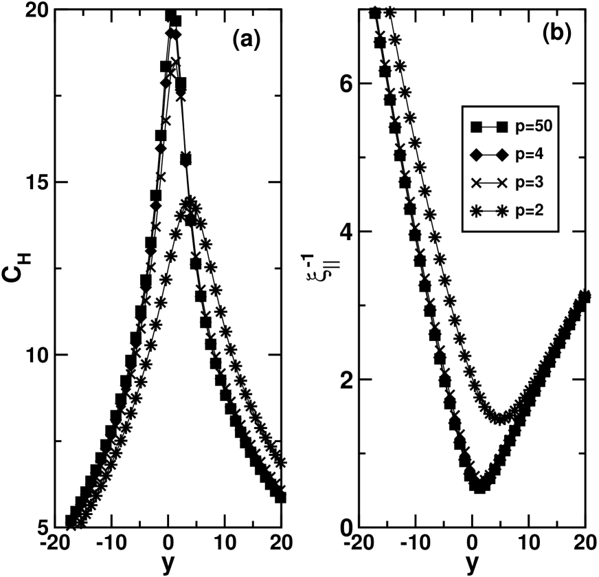
Figure 5: (a) Specific heat $C_{H}$ (in units of $k_{B}$) and (b) the inverse longitudinal spin-spin correlation length $\xi_{\parallel}^{-1}$ for the same system as in Fig. 3 as a function of the scaling variable $y$ for $h_{1}\approx 8.16$ and various values of the parameter $p$ (represented by the same symbols for both quantities).

The change of the locus of the minimum of the solvation force as the parameter $p$ is varied is consistent with the behaviour of the specific heat $C_{H}(L,T;p,h_{1})=-T(\partial^{2}f/\partial T^{2})_{L}$ and of longitudinal spin-spin correlation length $\xi_{\parallel}$. These quantities are readily calculable from the total free energy obtained in DMRG. $\xi_{\parallel}$ may be expressed in terms of the ratio of the largest $\Lambda_{0}$ and second largest $\Lambda_{1}$ eigenvalues of the transfer matrix $\xi^{-1}_{\parallel}(L,T;p,h_{1})=-\ln[\lambda_{1}/\lambda_{0}]$. We have calculated $C_{H}$ and $\xi^{-1}_{\parallel}$ as a function of temperature for $L=100$, $h_{1}\approx 8.16$ and various $p$. Both quantities exhibit extrema above $T_{c}$ which decrease and shift towards higher values of $T$ as the range of the surface potential increases (see Fig. 5 a, b). If the position of the extrema of $f_{solv}(T)$, $C_{H}(T)$, and $\xi^{-1}_{\parallel}(T)$ at $h=0$ is governed by capillary condensation maciolek:01:0 (see Sec. II), then their shift towards higher values of $T$ indicates that the (capillary) critical point moves further away from the bulk coexistence line $h=0$ as the range of the surface potential increases.

III Analysis of Landau functional

In this section we analyse the Landau theory corresponding to the Ising model considered in Sec. II in order to understand why at high temperatures the solvation force is negative and, for large wall separation $L$, decays as $L^{-(p+1)}$, whereas at low temperatures $f_{solv}(L)$ is positive and the form of decay agrees with the prediction (5), i.e. $f_{solv}(L)\sim L^{-p},~{}~{}~{}L\to\infty$.

In the Landau theory the magnetization profile $m(z)$ in a slit of width $L$ subject to the boundary field $H(z)$ is obtained by minimizing the free-energy functional (per unit area and per $k_{B}T$) fisher:81:0 :

$$F[m]=\int_{0}^{L}dz\left[\frac{1}{2}b\left(\frac{dm}{dz}\right)^{2}+f_{b}(m(z))-H(z)m(z)\right]$$ (15)

where $b$ is a positive constant. $f_{b}(m)$ is the bulk free-energy density

$$f_{b}(m)=\frac{1}{2}a\tau m^{2}+\frac{1}{4}am^{4}-hm,$$ (16)

where $\tau$ is the reduced deviation from the bulk critical temperature, $a$ is constant and $h$ is the bulk magnetic field. We consider a long ranged boundary field $H(z)$ of the form

$$H(z)=h_{1}\left[\frac{1}{(z+\lambda)^{p}}+\frac{1}{(L+\lambda-z)^{p}}\right],$$ (17)

where we have introduced the parameter $\lambda$ satisfying $L\gg\lambda\gtrsim 1$ in order to assure that $H(z)$ is well behaved at the boundaries. In the final analysis we take the limit $\lambda/L\to 0$.

In order to obtain the solvation force one has to find the equilibrium magnetization profile $m(z)_{eq}$ and then calculate the total excess free energy per unit area

$$f_{ex}(L)\equiv F(L)-Lf_{b}(m_{b}),$$ (18)

where $F(L)\equiv F[m_{eq}]$ and $m_{b}$ is the bulk magnetization at given $T,h$. The solvation force is defined by Eq. (10).

Henceforward, since we are interested in the asymptotic decay of $f_{solv}(L)$ for temperatures above $T_{c}$ and at vanishing bulk magnetic field, for our analysis it is sufficient to keep only the term quadratic in $m$ in the expression for the bulk free energy density. In this temperature range the bulk correlation length $\xi_{b}=(b/a\tau)^{1/2}$ and $m_{b}=m^{*}=0$.

Minimization of Eq. (15) yields an Euler-Lagrange equation

$$\frac{d^{2}m(z)}{dz^{2}}=\xi_{b}^{-2}m(z)-(1/b)H(z).$$ (19)

We assume the following boundary conditions

$$m(0)=m(L)=1,$$ (20)

valid for the considered case, i.e. large $h_{1}$, strongly adsorbing walls. Imposing the condition that at equilibrium the profiles are symmetric around $z=L/2$ yields further

$$\frac{dm}{dz}_{z=L/2}=0.$$ (21)

The solution to the Euler-Lagrange equation (19) is equal to the sum of the general solution, $m_{g}(z)$, of the corresponding homogeneous differential equation (with $H(z)=0$), and any particular solution, $m_{p}(z)$, of the inhomogeneous equation (with $H(z)\neq 0$):

$$m(z)=m_{g}(z)+m_{p}(z).$$ (22)

Above $T_{c}$ the general solution of equation (19) with $H(z)=0$ satisfying the symmetry condition (21) is

$$m_{g}(z)=A\left[e^{-z/\xi_{b}}+e^{-(L-z)/\xi_{b}}\right].$$ (23)

The required solution of the inhomogeneous equation can be expressed in the form of a power series in $H(z)$

$$m_{p}(z)=B_{1}\left[\frac{1}{(z+\lambda)^{p}}+\frac{1}{(L+\lambda-z)^{p}}\right]+B_{2}\left[\frac{1}{(z+\lambda)^{p+2}}+\frac{1}{(L+\lambda-z)^{p+2}}\right]+\ldots$$ (24)

where the constants $B_{1},B_{2},\cdots$ have to be determined by equating coefficients. We substitute (24) for $m(z)$ and its second derivative in the differential equation (19) and notice that for large separation $L\to\infty$ the lhs of this equation is subdominant to the rhs. Therefore, in the limit $L\to\infty$, we can approximate $m_{p}(z)$ by the solution of the equation

$$0=\xi_{b}^{-2}m(z)-(1/b)H(z),$$ (25)

i.e., $m_{p}(z)\approx(\xi_{b}^{2}/b)H(z)$. Thus the general solution of (19) is

$$m(z)\approx A\left[e^{-z/\xi_{b}}+e^{-(L-z)/\xi_{b}}\right]+\frac{\xi_{b}^{2}}{b}H(z),$$ (26)

where the constant $A$ can be determined from the boundary conditions (20). Substituting the above solution into the functional (15), performing the integral over $z$ and then the derivative with respect to $L$, one can find the asymptotic behaviour of $f_{solv}(L)$ when $L\to\infty$. Notice, that for $T>T_{c}$ the bulk spontaneous magnetization $m^{*}=0$, so that $f_{b}(m_{b})=0$ in the Eq. (18) for the excess free energy per unit area.

Substitution of the equilibrium magnetization profile (26) into the integrand in (15) yields terms purely exponentially and purely algebraically decaying with $z$, as well as terms in which an exponential and an algebraic decay mixes together. There are no terms decaying in the same fashion as the boundary field. Such terms, if they were to exist, would yield the power-law decay of $f_{solv}$ that is consisitent with the result by Attard et al. (Eq. (5)). Careful analysis reveals that the leading asymptotic behavior of the solvation force arises from a purely algebraically decaying term in $(b/2\xi_{b}^{2})m^{2}(z)-H(z)m(z)$, namely

$$-\frac{\xi_{b}^{2}h_{1}^{2}}{b}\frac{1}{(\lambda+z)^{p}(L+\lambda-z)^{p}}.$$ (27)

The contribution to the $f_{solv}$ from the above term is (see Appendix)

$$\frac{\xi_{b}^{2}h_{1}^{2}}{b}\frac{\partial}{\partial L}\int_{0}^{L}dz\frac{1}{(\lambda+z)^{p}(L+\lambda-z)^{p}}=-\frac{2\xi_{b}^{2}h_{1}^{2}}{b\lambda^{p-1}}\frac{p}{p-1}\frac{1}{L^{p+1}}+O(L^{-(p+2)}),~{}~{}~{}L\to\infty.$$ (28)

Other purely algebraically decaying terms in $(b/2\xi_{b}^{2})m^{2}(z)-H(z)m(z)$ give contributions to the solvation force that are $O(L^{-(2p+1)})$ and the mixed terms cancel out.

Contributions to the solvation force arising from $(1/2)b\left(dm/dz\right)^{2}$ decay faster than $L^{-(p+1)}$ for $L\to\infty$. In this expression there are four mixed terms:

$$\frac{e^{-z/\xi_{b}}}{(z+\lambda)^{p+1}};~{}~{}~{}~{}~{}~{}~{}~{}~{}~{}~{}~{}~{}~{}~{}~{}\frac{e^{-(L-z)/\xi_{b}}}{(L+\lambda-z)^{p+1}}.$$ (29)

$$\frac{e^{-(L-z)/\xi_{b}}}{(z+\lambda)^{p+1}};~{}~{}~{}~{}~{}~{}~{}~{}~{}~{}~{}~{}~{}~{}~{}~{}\frac{e^{-z/\xi_{b}}}{(L+\lambda-z)^{p+1}}.$$ (30)

The asymptotic behaviour of contributions to the solvation force arising from the above terms is (see Appendix)

$$-\frac{\partial}{\partial L}\int_{0}^{L}dz\frac{e^{-z/\xi_{b}}}{(L+\lambda-z)^{p+1}}=-\frac{\partial}{\partial L}\int_{0}^{L}dz\frac{e^{-(L-z)/\xi_{b}}}{(\lambda+z)^{p+1}}=\frac{(p+1)\xi_{b}}{(L+\lambda)^{p+2}}+O(L^{-(p+3)}),~{}~{}L\to\infty$$ (31)

and

$$-\frac{\partial}{\partial L}\int_{0}^{L}dz\frac{e^{-z/\xi_{b}}}{(\lambda+z)^{p+1}}=-\frac{\partial}{\partial L}\int_{0}^{L}dz\frac{e^{-(L-z)/\xi_{b}}}{(L+\lambda-z)^{p+1}}=-\frac{e^{-L/\xi_{b}}}{(\lambda+L)^{p+1}}+\frac{1}{\lambda^{(p+1)}},~{}~{}L\to\infty.$$ (32)

Purely algebraically decaying terms in the expression $-(b/2)m(z)\left(d^{2}m/dz^{2}\right)$ give contributions $O(L^{-(p+2)})$.

In conclusion, we have found that for $T>T_{c}$

$$f_{solv}(L)=-\frac{2\xi_{b}^{2}h_{1}^{2}}{b\lambda^{p-1}}\frac{p}{p-1}\frac{1}{L^{p+1}}+O(L^{-(p+2)}),~{}~{}~{}L\to\infty.$$ (33)

Note that since $b>0$ the solvation force is negative. This asymptotic behaviour does not change if we take into account higher order terms in the solution for $m_{p}(z)$ (see Eq. (24)).

The fact that in the limit $L\to\infty$ the solvation force decays faster than the boundary field is due to the absence in the expression for the free energy density of terms proportional to $H(z)$. Below $T_{c}$ the solution of the Euler-Lagrange equation (Eq. (19) with an additional term $\tau^{-1}\xi_{b}^{-2}m^{3}(z)$ in the rhs ) for large $L$ has the form $m(z)=m^{\ast}+{\tilde{m}}(z)$, where $m^{\ast}\neq 0$ is the bulk spontaneous magnetization. Similarly to the case of $T>T_{c}$, the function ${\tilde{m}}(z)$ can be expressed as a sum of the solution of the corresponding homogeneous differential equation (with $H(z)=0$), $m_{h}(z)$, and a solution of the inhomogeneous equation (with $H(z)\neq 0$), $m_{inh}(z)$, i.e. ${\tilde{m}}(z)=m_{h}(z)+m_{inh}(z)$ . For large $L$ the approximation (26) for $m_{inh}(z)$ is still valid, therefore in the expression for the free energy we can expect terms $\sim m^{\ast}H(z)$ which then yield an asymptotic decay of the solvation force of the same form as that of the boundary field.

IV Density functional theory results

The model considered in this Section is a van der Waals fluid of the bulk density $\rho_{b}$ confined in a slit of width $L$. Each of the walls interacts with the fluid via the potential described by Eq. (3) with $p=2,3$. The total external potential of the system $V_{ext}(z)$ is a sum of the contributions from both walls, $V_{ext}(z)=V_{s}(z)+V_{s}(L-z)$. The fluid particles interact via the standard Lennard–Jones potential

$$u(r)=\left\{\begin{array}[]{ll}4\varepsilon_{ff}\left[\left(\frac{\sigma}{r}\right)^{12}-\left(\frac{\sigma}{r}\right)^{6}\right]\;,&r<r_{cut}\\ 0\;\;,&r>r_{cut}\end{array}\right.$$ (34)

where $\varepsilon_{ff}$ describes the strength of the fluid–fluid interactions and $r_{cut}$ is the cut-off distance. We set $r_{cut}=2.5\sigma$. The system is studied by means of a density functional theory (DFT) Evans92 . Within this approach the grand potential $\Omega$ of the system is a functional of the local density $\rho({\bf r})$

$$\Omega[\rho]=F[\rho]+\int d^{3}r\,\rho({\bf r})(V_{ext}({\bf r})-\mu)$$ (35)

where $\mu$ is the chemical potential of the fluid. The free energy functional $F$ is a sum of two parts, $F=F_{id}+F_{ex}$. The ideal gas contribution is known exactly

$$\beta F_{id}=\int d^{3}r\,[\ln(\Lambda^{3}\rho({\bf r})-1]\rho({\bf r})\;,$$ (36)

where $\beta=(k_{B}T)^{-1}$ and $\Lambda$ is the de Broglie wavelength. The excess (over ideal) free energy is a sum of reference hard–sphere $F_{ex}^{(hs)}$ and attractive $F_{ex}^{(att)}$ contributions. The latter is evaluated in a mean–field fashion

$$F_{ex}^{(att)}=\frac{1}{2}\int d^{3}r\int d^{3}r^{\prime}\,\rho({\bf r})\rho({\bf r}^{\prime})u_{WCA}(|{\bf r}-{\bf r}^{\prime}|)\;$$ (37)

where $u_{WCA}(r)$ corresponds to the Weeks-Chandler-Andersen Weeks79 division of the interparticle potential

$$u_{WCA}(r)=\left\{\begin{array}[]{ll}-\varepsilon_{ff}\;,&r<2^{\frac{1}{6}}\sigma\\ u(r)\;,&r>2^{\frac{1}{6}}\sigma\end{array}\right.$$ (38)

The reference hard–sphere part of the excess free energy is evaluated within the framework of the Fundamental Measure theory (FMT) of Rosenfeld Rosenfeld89 ; Rosenfeld93

$$\beta F_{ex}^{(hs)}=\int d^{3}r\;\Phi(\{n_{\alpha}\})\;,$$ (39)

where $n_{\alpha}$ denote weighted densities

$$n_{\alpha}({\bf r})=\int d^{3}r^{\prime}\rho({\bf r}^{\prime})~{}w_{\alpha}({\bf r}-{\bf r}^{\prime})\;,$$ (40)

with six different geometrical weight functions $w^{(\alpha)}$ (four scalar and two vector–like Rosenfeld93 ). There are several expressions for the excess free energy density $\Phi$. We have chosen for the present problem the original Rosenfeld functional, where the excess free energy density is given by

$$\Phi(\{n_{\alpha}\})=-n_{0}\ln(1-n_{3})+\frac{n_{1}n_{2}-{\bf n}_{1}\cdot{\bf n}_{2}}{1-n_{3}}+\frac{n_{2}^{3}-3n_{2}{\bf n}_{2}\cdot{\bf n}_{2}}{24\pi(1-n_{3})^{2}}\;.$$ (41)

The density profile $\rho({\mathbf{r}})\equiv\rho(z)$, for planar walls, is obtained by solving the Euler–Lagrange equation, i.e. from

$$\frac{\delta\Omega}{\delta\rho({\bf r})}=0\;.$$ (42)

The solvation force ${\tilde{f}}_{solv}(L)$ (or excess pressure) can be obtained from

$${\tilde{f}}_{solv}=-\frac{1}{A}\left(\frac{\partial\Omega_{ex}}{\partial L}\right)$$ (43)

where $A$ denotes the area of the wall and $\Omega_{ex}\equiv\Omega+pV$ is the excess grand potential of the system. Here $p$ is the pressure of the reservoir at the chemical potential $\mu$ and the bulk density $\rho_{b}$ and $V$ is the total volume. Statistical mechanical sum rules Henderson92 for a confined fluid lead to another expression for the solvation force

$${\tilde{f}}_{solv}=-p-\int_{-\infty}^{\infty}dz\rho(z)\frac{\partial}{\partial z}V_{s}(z)$$ (44)

We have used the above equation to check the accuracy of the numerics.

Without loss of generality we chose the LJ $\sigma$ as a unit of length, and introduce the following reduced units, $f_{solv}=\beta{\tilde{f}}_{solv}\sigma^{3}$, $T^{\ast}=\frac{k_{B}T}{\varepsilon_{ff}}$, $\rho^{\ast}_{b}=\rho_{b}\sigma^{3}$. For the system in question the reduced critical temperature and the reduced critical density for the gas-liquid transition are $T_{c}^{\ast}=1.319442$ and $\rho_{c}^{\ast}=0.245736$, respectively.

We start by reporting the temperature dependence of the rescaled solvation force $f_{solv}^{\ast}$, i.e. the solvation force divided by its value at $T/T_{c}=0.615$, for systems with $p=3,2$ and $L=50.4\sigma$ (see Fig. 6). In analogy with the results presented in Sec. II.3 the chemical potential $\mu(T)$ (or, equivalently the bulk density of the reservoir, $\rho_{b}^{\ast}$) is fixed such that the bulk fluid is slightly off coexistence on the liquid side of the bulk coexistence curve. We notice that for the system with the wall-fluid interactions of the finite range, i.e. for truncated wall-fluid potential (3) with $p=3$ and cut-off $z=2.5\sigma$, (see the inset) the solvation force is extremaly small away from $T_{c}$. At low temperature the system is on the oscillatory side of the Fisher-Widom line, so the solvation force should decay in an exponentially-damped oscillatory fashion i.e. $f_{solv}(L\to\infty)$ $\sim\exp(-a_{0}L)\cos(a_{1}L)$ dijkstra:00:0 . Consequently, for the large separations considered here the solvation force well below $T_{c}$ becomes extremely small in magnitude and perishes in the numerical noise, i.e. its magnitude is smaller than $10^{-10}$. Close to the critical region a pronounced decrease in the solvation force is found (see the inset) with its minimum located slightly above $T_{c}$. Note that for $T>T_{c}$ we follow the critical isochore $\rho_{b}(\mu,\tau)=\rho_{c}$ and the decay is expected to be purely exponential, at least in the range shown in Fig. 6. For this value of $L$ the magnitude is extremely small.

For the systems with long ranged wall-fluid potentials we find that for $p=3$ (Fig. 6, solid line) the solvation force is positive away from the critical region. Only very close to $T_{c}$ does $f_{solv}^{\ast}$ change sign and become negative. The minimum is located slightly above $T_{c}$. For still stronger fluid-wall potentials i.e. for $p=2$ (Fig. 6, dashed line) the solvation force is positive (repulsive) through the entire range of temperatures under consideration. The rescaled solvation force is almost identical for both values of $p$ at temperatures away from $T_{c}$ which is consistent with the result of Eq. (5), i.e. $f_{solv}^{\ast}\sim\rho(T)$ . As the systems move towards the critical region, $f_{solv}^{\ast}$ begins to be different for different powers of the wall-fluid potentials. However the minimum of $f_{solv}^{\ast}$ is located, similarly to previous cases, slightly above the critical temperature. These findings are in accordance with general considerations presented in the Introduction. The minimum of the solvation force is connected with the critical Casimir effect krech:99:0 . For short ranged wall-fluid potentials this effect is dominant (see the inset to Fig.  6) as the direct influence of the wall is negligible at large separations. When the long ranged wall-fluid potentials are introduced, the contribution from the regular part of the solvation force $f_{solv}^{reg}$ , which is different for different powers of the wall-fluid potential, dominates for temperatures away from the $T_{c}$ while for systems in the critical region the singular part of the solvation force $f_{solv}^{sing}$ comes into play. The dominant decay of the singular part is the same for both value of $p$. In the present DFT approach the critical Casimir force is treated in mean-field, therefore $f_{solv}^{sing}$ is given by (11) with $d=4$ and the mean-field value of the exponent $\nu$ ($\nu_{MF}=1/2$).

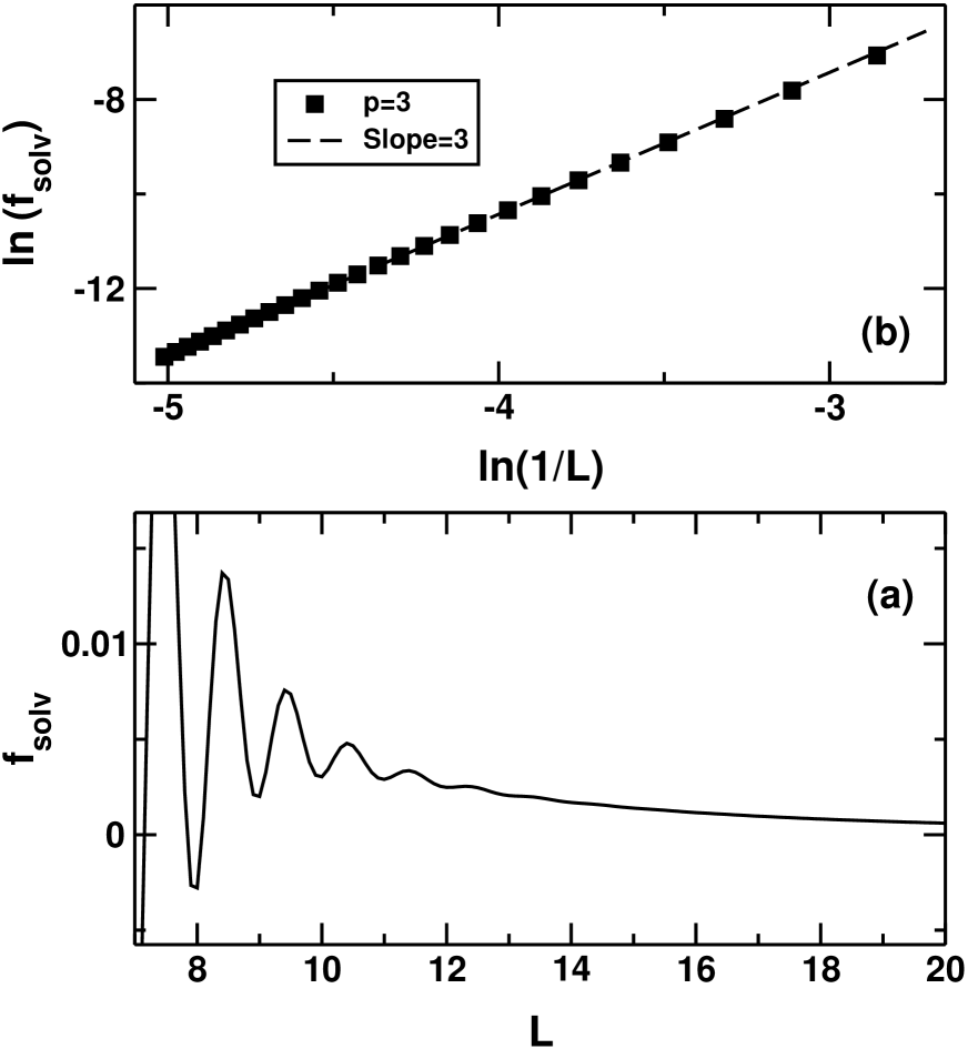
Figure 7: The oscillatory (part a) and asymptotic shown on a $\log-\log$ plot (part b) regions of the solvation force for the system with $p=3$ evaluated from density functional theory. The temperature ($T^{\ast}=1.0$) and the reservoir density ($\rho_{b}^{\ast}=0.6148$) are fixed such that the fluid is just slightly off the coexistence on the liquid branch of the coexistence curve.

In Figs. 7-8 we show the $L$-dependence of the solvation force for systems with long-range wall-fluid potentials for the bulk reservoir state $T^{\ast}=1.0$, $\rho_{b}^{\ast}=0.6148$. Again the temperature and chemical potential were fixed such that the system is just slightly away from coexistence on the liquid branch of the coexistence curve. We observe that for intermediate $L$ the well-known oscillatory behaviour of $f_{solv}$ characteristic, for short separations, is damped and changes gradually to the power-law decay enforced by the external (long ranged) wall-fluid potential. The asymptotic behaviour of the solvation force is demonstrated in Fig. 7b and Fig. 8b, where we plot the logarithm of $f_{solv}$ as a function of the logarithm of the inverse separation (symbols) along with best straight line fits with imposed slope (solid lines) for the systems with $p=3$, and $2$, respectively. These are similar to these in Fig. 3, presented in Sec. II.3. In both cases we find a nice agreement between the DFT results and the predictions from Eq. (5). The asymptotic form of the decay is quite visible already for medium separations, i.e. for $L>50$. In order to investigate further the asymptotic behaviour of the solvation force we have performed least-square fits assuming a power-law, i.e. assuming $f_{solv}(L)=a_{0}L^{\kappa}$ with $a_{0},\kappa$ taken as fit parameters. For the system presented in Figs. 7-8 best fits performed for $190>L>110$ are $4.69x^{-2.99}$ and $4.62x^{-1.99}$, respectively, where $x=L/\sigma$. The value of the constant $a_{0}$ predicted by Eq. (5) is 4.92 and differs from those given by least-square fits by $\sim 6\%$. We also note that the constant $a_{0}$ should be the same for both potentials considered here (it depends on only the density $\rho_{b}^{\ast}$ and the parameter $B=4\varepsilon f_{w}$ which is same for both) and indeed, to a good approximation, this is the case here.

It has been well established evans:86:0 ; evans:87:0 that if the chemical potential is fixed such that the fluid is on the gas side of the liquid-gas phase diagram the solvation force can (as a function of the separation) exhibit a jump that is a direct manifestation of capillary condensation. The discontinuity can appear for both short ranged and long ranged wall-fluid potentials. If the wall-fluid interactions are short ranged, $f_{solv}(L)$ will change from small negative (weakly attractive) values at large $L$ (corresponding to the ’gas’ phase) to larger negative values for smaller $L$ (corresponding to the ’liquid’ phase). As argued in the Ref. evans:87:0 on the basis of macroscopic thermodynamic arguments there is always the term $-\Delta\mu(\rho_{l}-\rho_{g})$ in the expression for $f_{solv}$ for the capillary condensed ’fluid’ which gives rise to the aforementioned jump. On the basis of the theory of the asymptotic decay of the correlation functions evans:93:0 ; evans:94:1 it was argued that the solvation force should decay (asymptotically) in the same manner as the bulk pair correlation function. In the present case the fluid lies on the monotonic side of the Fisher-Widom line. A schematic plot of $f_{solv}$ is shown in Fig. 9a (for clarity the oscillatory part of the solvation force, relevant for small separations is omitted here).

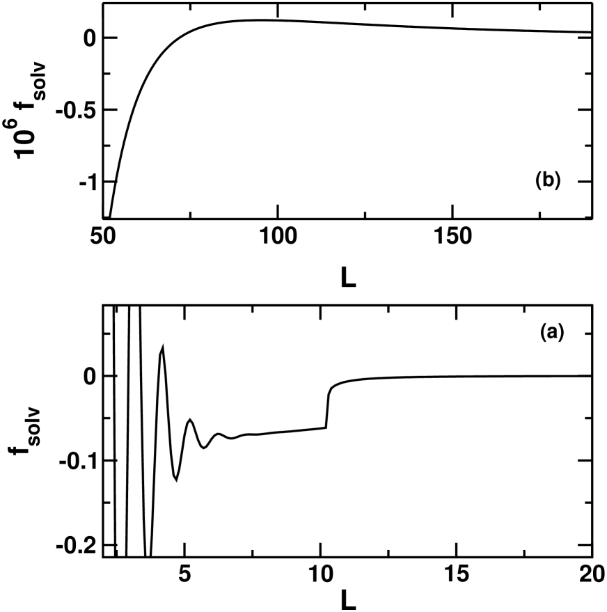
Figure 10: The short distance (part a) and asymptotic (part b) regions of the solvation force for the system with long ranged ($p=3$) wall-fluid interactions. Note the change of scale in each part. Capillary condensation gives rise to the jump at $L=10.5$. For $L<10.5$ the confined fluid is a ’liquid’ which can exhibit oscillations. The bulk reservoir corresponds to ($T^{\ast}=1.2$, $\rho_{b}^{\ast}=0.06$).

When the wall-fluid interactions become long ranged the solvation force should decay asymptotically in the same fashion as the wall-fluid potential because its contribution to the $f_{solv}$ will be dominant with respect to the fast-decaying (exponential) fluid-fluid contribution. On the other hand, the discontinuity in $f_{solv}$ connected with capillary condensation must remain. Thus one can anticipate that the solvation force should behave in the manner presented in Fig. 9b (again, for clarity the oscillatory part of the solvation force, relevant for small separations is omitted here). Namely, upon increasing the wall-wall separation $L$, the solvation force jumps from larger to smaller but still negative values. This discontinuity is associated with capillary condensation. Next, $f_{solv}$ changes its sign (the point denoted by $Z$), attains a maximum (the point denoted by $M$) followed by the inflection point (denoted by $I$) and, finally, reaches the region of the asymptotic decay dictated by Eq. (5). The specific example of the solvation force calculated by DFT for the system with $p=3$, $T^{\star}=1.2$ and $\rho^{\star}_{b}=0.06$ shown in Fig. 10 fits well into the general behaviour described above. The jump associated with the capillary condensation occuring at $L\sim 10.5$ (c.f. Fig. 10a) is from larger to smaller but still negative values of $f_{solv}$. As the wall-wall separation is increased (c.f. Fig. 10b) $f_{solv}$ changes its sign around $L\sim 72$, attains a maximum at $L\sim 95$. After an inflection point at $L\sim 130$ the solvation force changes slowly towards its asymptotic form of decay. It must be mentioned however that even for the largest separation studied ($L=190$) the asymptotics (i.e. the decay with a power-law the same as the decay of the wall-fluid potential) could not be still reached. We think one needs to go to the separations as large as several hundreds to rich the asymptotic range.

V Summary and Conclusions

In this paper we have performed calculations of the solvation force for an Ising film subject to long ranged boundary fields (2) with $p=50,4,3$, and 2, and for a truncated LJ fluid confined between two planar walls that exert a $9-p$ with $p=2,3$ wall-fluid potential (3). For an Ising film results have been obtained in $d=2$ for states along the line of the bulk two-phase coexistence $h=0$ by means of the DMRG method which takes into account fluctuations of the order parameter. Since in two dimensions critical fluctuations are particularly strong, results obtained in this model serve as an ultimate test of the effects of fluctuations on the behaviour of the solvation force. For LJ fluid results have been obtained for several states on a liquid side of the bulk two-phase coexistence and on the critical isochore for $T>T_{c}$ within a nonlocal DFT which is a mean field theory. This approach accounts for packing effects and hence oscillations in the solvation force.

We observe major differences in the behaviour of the solvation force between the both models. In the Ising system $f_{solv}$ at low temperatures is positive (repulsive) and decays for large $L$ in the same fashion as the boundary field, i.e., $f_{solv}=L^{-p}$, whereas at high temperatures $f_{solv}$ is negative (attractive) and the asymptotic decay is of the higher order than that of the boundary field, i.e., $f_{solv}=L^{-(p+1)}$. In the LJ fluid system $f_{solv}$ is always repulsive away from the critical region and decays for large $L$ with the the same power law as the wall-fluid potential, which is consistent with the general result (5) based on the wall-particle Ornstein-Zernike equations attard:91:0 . As discussed within a Landau approach in the Sec. III the origin of this discrepancy is due to the specific symmetry of the Ising model with the spontaneous magnetization $m^{\ast}$ equal to zero above $T_{c}$; note that for a fluid $\rho_{c}(T)\neq 0$ above $T_{c}$.

Our results imply that for a confined fluid with short ranged fluid-fluid interactions and long ranged wall-fluid potential the solvation force, for large wall separations, can be expressed as a sum of a regular part $f_{solv}^{reg}$, which decays in the same fashion as the wall-fluid potential, and a part $f_{solv}^{sing}$ arising from L-dependent singular contribution krech:99:0 to the free energy, which is a close analog of the Casimir force in electromagnetism. The singular contribution to the free energy is responsible for the critical singularities at the bulk critical point. Thus, for ordering field $h=0$ and $L\to\infty$

$$f_{solv}\sim f_{solv}^{reg}+f_{solv}^{sing}=2\rho BL^{-p}+(d-1)L^{-d}W_{aa}(\tau L^{1/\nu})$$ (45)

where $W_{aa}(y)$ is a finite-size scaling function for system with two identical walls $a$, and $B=4\varepsilon_{fw}$ for a wall-fluid potential of a form (3). In mean-field $d$ takes the value 4 in the final term of Eq. (45). Such a decomposition applies also for an Ising spins system below $T_{c}$ with $\rho B$ replaced by $m^{\ast}h_{1}$. Above $T_{c}$, $m^{\ast}$ vanishes and the leading regular part of the solvation force becomes $\sim L^{-(p+1)}$ as already mentioned above. The scaling function $W_{aa}(y)$ is negative and vanishingly small away from the critical region, therefore, in $d=2$ and 3 and for all values of the parameter $p$ the positive regular part of the solvation force dominates away from $T_{c}$. Fluctuation induced attractive Casimir force is particularly strong in two dimensions and dominates the behaviour of the solvation force in the critical region for all considered values of the parameter $p$ - see Fig. 1. In mean field $f_{solv}^{sing}$ is much weaker and only when $p\geq d=3$ the solvation force becomes weakly negative near $T_{c}$. For $p=2$ the regular part $f_{solv}^{reg}$ gives the leading decay and although the solvation force exhibits minimum near $T_{c}$, it remains positive for all temperatures as is seen in Fig. 6.

As a last remark we note that the inclusion of power-law fluid-fluid interactions would modify our results. This can be infered from the asymptotic integral equation results for the solvation force of the full LJ fluid - see Eq. (4). The final term is associated with the $-r^{-n}$ decay of the fluid-fluid potential. For LJ $n=6$ so Eq. (4) predicts an additional attractive term $\sim L^{-3}$ in the solvation force. This should then be included in Eq. (45). This contribution competes with other terms and may lead to even richer behaviour of the solvation force. We want to stress that in our studies we have neglected the contribution due to the direct wall-wall interaction potential footnote .

After the completion of our calculations we learnt of a recent article by Pertsin and Grunze pertsin:03:0 describing the results of Monte Carlo simulations of a Lennard-Jones fluid confined between two planar walls. Since their results were at complete variance with ours and with the general predictions of Eq. (4) we decided to perform DFT calculations for the same state point as in the simulations of Ref. pertsin:03:0 . The results are presented in Appendix B. As expected, we find no evidence for the extremely long ranged solvation force reported in Ref. pertsin:03:0 . We have since ascertained, via correspondence with Professor A. Pertsin and Professor R. Evans, that the simulations reported in Ref. pertsin:03:0 were flawed and that the authors shall publish an erratum pointing this out. The new results, however, are in a good qualitative agreement with our DFT results.

*

Appendix A A

In order to evaluate contributions to the solvation force arising from terms (27), (29) and (30) we use Eqs. (10), (18), and  (15).

First we integrate over $z$ to obtain contributions to the total free energy. We find grad

$$\int_{0}^{L}\frac{dz}{(\lambda+z)^{p}(L+\lambda-z)^{p}}=\frac{L}{2p-1}\sum_{k=0}^{p-2}\frac{2^{k+1}(2p-1)(2p-3)\cdots(2p-1-2k)}{(p-1)(p-2)\cdots(p-k-1)\Delta^{k+1}(L\lambda+\lambda)^{p-k-1}},$$ (46)

where $\Delta=(4L\lambda+4\lambda+L^{2})$. In the limit of $L\to\infty$ and $\lambda/L\to 0$ the above integral simplifies

$$\int_{0}^{L}\frac{dz}{(\lambda+z)^{p}(L+\lambda-z)^{p}}\to_{L\to\infty}\sum_{k=0}^{p-2}\frac{2^{k+1}(2p-3)\cdots(2p-1-2k)}{(p-1)(p-2)\cdots(p-k-1)\lambda^{p-k-1}L^{p+k}}.$$ (47)

It follows that the contribution to the solvation force arising from the term (27) is

$$\frac{\xi_{b}^{2}h_{1}^{2}}{b}\frac{\partial}{\partial L}\int_{0}^{L}dz\frac{1}{(\lambda+z)^{p}(L+\lambda-z)^{p}}=-\frac{2\xi_{b}^{2}h_{1}^{2}}{b\lambda^{p-1}}\frac{p}{p-1}\frac{1}{L^{p+1}}+O(L^{-(p+2)}),~{}~{}~{}L\to\infty.$$ (48)

Integration of terms (29) yields

$$\int_{0}^{L}dz\frac{e^{-z/\xi_{b}}}{(L+\lambda-z)^{p}}=\int_{0}^{L}dz\frac{e^{-(L-z)/\xi_{b}}}{(\lambda-z)^{p}},$$ (49)

and

$$\int_{0}^{L}dz\frac{e^{-z/\xi_{b}}}{(L+\lambda-z)^{p}} = \frac{1}{\xi_{b}^{p-1}(p-1)!}\sum_{k=1}^{p-1}\xi_{b}^{k}(k-1)!\left[\frac{e^{-L/\xi_{b}}}{\lambda^{k}}-\frac{1}{(L+\lambda)^{k}}\right]$$ (50)

$$+ \frac{1}{\xi_{b}^{p-1}(p-1)!}e^{-(L+\lambda)/\xi_{b}}\left[Ei(\frac{L+\lambda}{\xi_{b}})-Ei(\frac{\lambda}{\xi_{b}})\right],$$

where $Ei(x)$ is the Exponential-Integral Function.

An asymptotic representation of the function $Ei(x)$ for large $x$ is grad

$$e^{-x}Ei(x)=\sum_{k=1}^{n}\frac{(k-1)!}{x^{k}}+O(x^{-(n+1)})~{}~{}~{}~{}(x\to\infty).$$ (51)

Thus, in a limit of large $L$, the second term in the expression for the integral (50) behaves as

$$\frac{1}{\xi_{b}^{p-1}(p-1)!}e^{-(L+\lambda)/\xi_{b}}\left[Ei(\frac{L+\lambda}{\xi_{b}})-Ei(\frac{\lambda}{\xi_{b}})\right] =$$

$$\frac{1}{\xi_{b}^{p-1}(p-1)!}\left[\sum_{k=1}^{n}\xi_{b}^{k}(k-1)!\frac{1}{(L+\lambda)^{k}}-Ei(\frac{\lambda}{\xi_{b}})\right] + O((L+\lambda)^{-(n+1)})~{}~{}~{}(L\to\infty).$$ (52)

Using the above asymptotic expression we obtain the asymptotic behaviour of the integral (50) in a limit of $L\to\infty$

$$\int_{0}^{L}dz\frac{e^{-z/\xi_{b}}}{(L+\lambda-z)^{p}} = \frac{e^{-L/\xi_{b}}}{\xi_{b}^{p-1}(p-1)!}\left[\sum_{k=1}^{p-1}\xi_{b}^{k}(k-1)!\frac{1}{\lambda^{k}}-e^{-\lambda/\xi_{b}}Ei(\frac{\lambda}{\xi_{b}})\right]$$ (53)

$$+ \frac{\xi_{b}}{(L+\lambda)^{p}}+O(L^{-(p+1)}).$$

It follows that

$$-\frac{\partial}{\partial L}\int_{0}^{L}dz\frac{e^{-z/\xi_{b}}}{(L+\lambda-z)^{p}} = \frac{e^{-L/\xi_{b}}}{\xi_{b}^{p}(p-1)!}\left[\sum_{k=1}^{p-1}\xi_{b}^{k}(k-1)!\frac{1}{\lambda^{k}}-e^{-\lambda/\xi_{b}}Ei(\frac{\lambda}{\xi_{b}})\right]$$ (54)

$$+ \frac{p\xi_{b}}{(L+\lambda)^{p+1}}+O(L^{-(p+2)})~{}~{}~{}~{}(L\to\infty).$$

Now, consider contributions to the solvation force arising from terms

$$\frac{e^{-z/\xi_{b}}}{(\lambda+z)^{p}};~{}~{}~{}~{}~{}~{}~{}~{}~{}~{}~{}~{}~{}~{}~{}~{}\frac{e^{-(L-z)/\xi_{b}}}{(L+\lambda-z)^{p}}.$$ (55)

We have

$$\int_{0}^{L}dz\frac{e^{-z/\xi_{b}}}{(\lambda+z)^{p}}=\int_{0}^{L}dz\frac{e^{-(L-z)/\xi_{b}}}{(L+\lambda-z)^{p}}$$ (56)

and

$$-\frac{\partial}{\partial L}\int_{0}^{L}dz\frac{e^{-z/\xi_{b}}}{(\lambda+z)^{p}}=-\frac{e^{-L/\xi_{b}}}{(\lambda+L)^{p}}+\frac{1}{\lambda^{p}}.$$ (57)

Appendix B B

In order to compare with the results of Ref. pertsin:03:0 we carried out DFT calculations for $T^{\ast}=1.0$ and $\rho^{\ast}_{b}=0.6853$, the simulation state point. In Ref. pertsin:03:0 the LJ potential is cut-off at $r_{cut}=2.5\sigma$, the same as in our DFT, and the wall-fluid potentials have the same form as (3). Fig. 11a shows our results for $f_{solv}(L)$ for the case of a 9-3 wall-fluid potential, i.e. $p=3$, whilst Fig. 11b refers to the truncated 9-4 wall-potential, set to zero at $z=2.5\sigma$. In the first case we confirmed that for large $L$, $f_{solv}(L)$ is positive and decays as $L^{-3}$. Indeed the fit to this power law is as good as that for the neighbouring state point shown in Fig. 7. For the truncated 9-4 potential $f_{solv}(L)$ exhibits the expected exponentially damped oscillatory decay for large $L$. Thus our results for this state point are also in agreement with the general theory described in the Introduction. By contrast Pertsin and Grunze pertsin:03:0 find for large $L$ an attractive solvation force which decays very slowly, roughly as $L^{-1}$, for both the 9-3 and the truncated 10-4 wall-fluid potentials (see their Fig. 3a). Such behaviour would seem to be unphysical.

Figure Captions

• Fig.1 Solvation force (in units of $J$) for an Ising strip of the width $L=300$ at vanishing bulk magnetic field subject to long ranged boundary fields $H_{l}=H^{s}_{l}+H^{s}_{L+1-l}$, $H^{s}_{l}=h_{1}/l^{p}$ as a function of the scaling variable $y\equiv\tau(L)^{1/\nu}=\tau L$ for various values of $p$ and the amplitude $h_{1}\approx 8.16$ calculated using DMRG method. The inset shows, on an expanded scale, that results for $p=50$ and $p=4$ differ only very slightly in the near-critical region. For all values of $p$ $~{}f_{solv}$ is attractive above $T_{c}$ and, except for $p=50$, repulsive below $T_{c}$.

• Fig.2 Log-log plot of the solvation force (in units of $J$) versus $1/L$ for two values of the power $p$ describing the decay of the boundary field $H^{s}_{l}$, $p=2$ and 4. (a) displays DMRG results for $T=0.79T_{c}$ (filled symbols) and $T=T_{c}$ (unfilled symbols). Straight lines correspond to $f_{solv}(L)\sim L^{-p}$. Data at $T_{c}$ align parallel to the line of a slope 2 showing the result $f_{solv}(L)\sim L^{-d}$ (see Eq. (1)) with $d=2$. (b) displays DMRG results for $T=1.23T_{c}$. Straight lines correspond to $f_{solv}(L)\sim L^{-(p+1)}$.

• Fig.3 Solvation force for the Ising strip of width $L=100$, $h_{1}\approx 8.16$ rescaled with its value at $T/T_{c}=0.75$, plotted as a function of the reduced temperature. Below $T_{c}$, the results calculated for three different values of the power $p$ lie on a common curve $\sim m^{*}(T/T_{c})$, where $m^{*}(T)$ is bulk spontaneous magnetization. This behaviour agrees with the prediction Eq. (5) with $2\rho B$ replaced by $2m^{*}(T)h_{1}$.

• Fig.4 Solvation force (in units of $J$) for the same system as in Fig. 3 as a function of the variable $y$ for a selection of values of the strength parameter $h_{1}$ and for two values of the parameter $p$: (a) $p=50$ and (b) $p=2$. Results for different values of $h_{1}$ in Fig. 4b are represented by the same symbols as in Fig. 4a. It is seen that the symmetry, Eq. (12) between $f_{solv}(y)$ for the free ($h_{1}=0$) and $(++)$ ($h_{1}\sim 8.16$) boundary conditions breaks when the boundary fields become long ranged. For weak $h_{1}$ the solvation force exhibit two minima.

• Fig.5 (a) Specific heat $C_{H}$ (in units of $k_{B}$) and (b) the inverse longitudinal spin-spin correlation length $\xi_{\parallel}^{-1}$ for the same system as in Fig. 3 as a function of the scaling variable $y$ for $h_{1}\approx 8.16$ and various values of the parameter $p$ (represented by the same symbols for both quantities).

• Fig.6 Solvation force rescaled with its value at $T/T_{c}=0.615$, $f_{solv}^{\ast}\equiv f_{solv}(T/T_{c})/f_{solv}(0.615)$, as a function of the temperature for systems with long ranged fluid-wall potentials for $L=50.4\sigma$ evaluated from density functional theory. The chemical potential $\mu(T)$ is chosen so that the reservoir density bulk density $\rho_{b}^{\ast}(T)$ is close to that of the bulk coexisting liquid for $T<T_{c}$ and $\rho_{b}(\mu,T)=\rho_{c}$ for $T\geq T_{c}$. Solid line corresponds to the system with $p=3$, while dashed line is for the system with $p=2$. The inset shows the temperature dependence of $f_{solv}$ for the system with fluid-wall interactions of the finite range.

• Fig.7 The oscillatory (part a) and asymptotic shown on a $\log-\log$ plot (part b) regions of the solvation force for the system with $p=3$ evaluated from density functional theory. The temperature ($T^{\ast}=1.0$) and the reservoir density ($\rho_{b}^{\ast}=0.6148$) are fixed such that the fluid is just slightly off the coexistence on the liquid branch of the coexistence curve.

• Fig.8 The oscillatory (part a) and asymptotic shown on a $\log-\log$ plot (part b) regions of the solvation force for the system with $p=2$ evaluated from density functional theory. The temperature ($T^{\ast}=1.0$) and the reservoir density ($\rho_{b}^{\ast}=0.6148$) are fixed such that the fluid is just slightly off the coexistence on the liquid branch of the coexistence curve. Note that for $p=2$ the solvation force has more pronounced oscillations than for $p=3$.

• Fig.9 Schematic plot of the solvation force for systems with short ranged (part a) and long ranged (part b) fluid-wall interactions in the presence of capillary condensation. Dots denoted by $Z,M$ and $I$ in part b mark characteristic points of the solvation force: the zero, the maximum and the inflection point, respectively.

• Fig.10 The short distance (part a) and asymptotic (part b) regions of the solvation force for the system with long ranged ($p=3$) wall-fluid interactions. Note the change of scale in each part. Capillary condensation gives rise to the jump at $L=10.5$. For $L<10.5$ the confined fluid is a ’liquid’ which can exhibit oscillations. The bulk reservoir corresponds to ($T^{\ast}=1.2$, $\rho_{b}^{\ast}=0.06$).

• Fig.11 Solvation force for the LJ fluid with the short ranged and long ranged wall-fluid potentials calculated within DFT for $T^{\ast}=1.0$ and $\rho^{\ast}_{b}=0.6853$, the same state point as in the simulations by Pertsin and Grunze pertsin:03:0 . (a) is for the full 9-3 LJ potential. Oscillations characteristic for short wall-wall separations are gradually damped and changed into the power law asymptotic decay. (b) is for the truncated 9-4 LJ potential with the cut-off distance 2.5$\sigma$. Oscillations around 0 are present for all wall-wall separations.

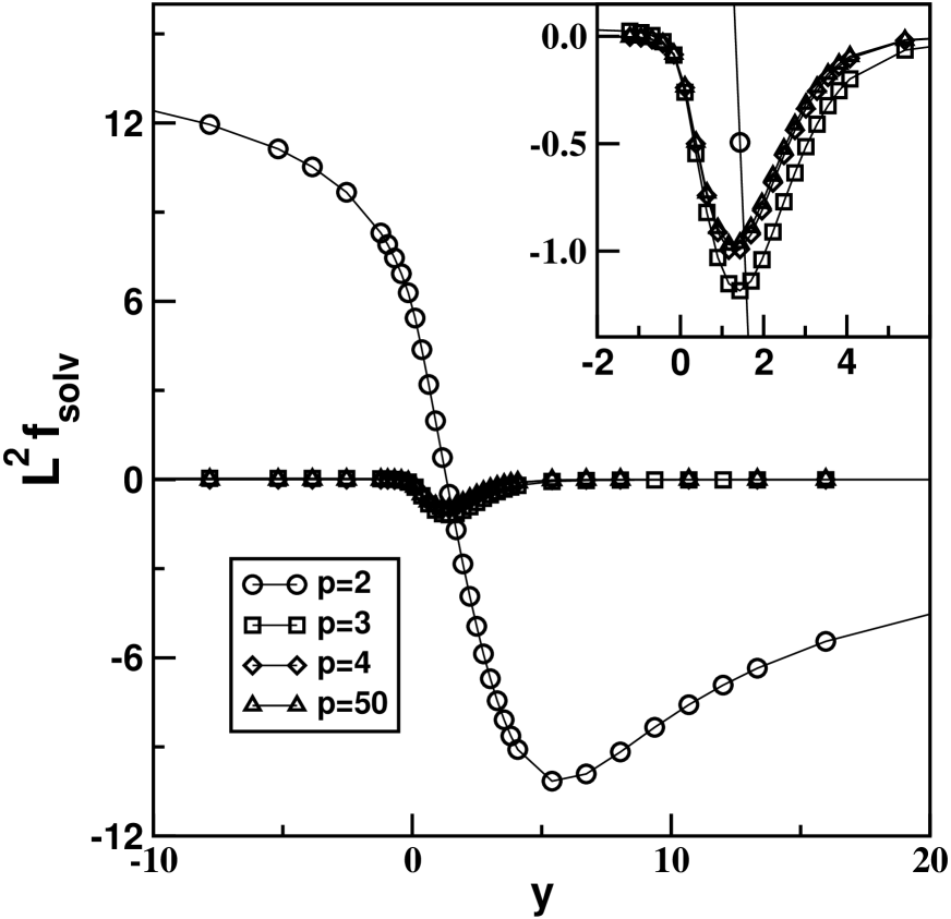
Figure 1: Solvation force (in units of $J$) for an Ising strip of the width $L=300$ at vanishing bulk magnetic field subject to long ranged boundary fields $H_{l}=H^{s}_{l}+H^{s}_{L+1-l}$, $H^{s}_{l}=h_{1}/l^{p}$ as a function of the scaling variable $y\equiv\tau(L)^{1/\nu}=\tau L$ for various values of $p$ and the amplitude $h_{1}\approx 8.16$ calculated using DMRG method. The inset shows, on an expanded scale, that results for $p=50$ and $p=4$ differ only very slightly in the near-critical region. For all values of $p$ $~{}f_{solv}$ is attractive above $T_{c}$ and, except for $p=50$, repulsive below $T_{c}$.

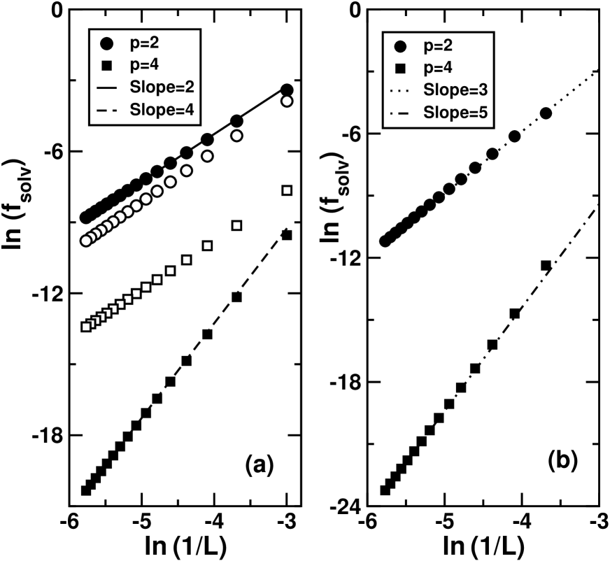
Figure 2: Log-log plot of the solvation force (in units of $J$) versus $1/L$ for two values of the power $p$ describing the decay of the boundary field $H^{s}_{l}$, $p=2$ and 4. (a) displays DMRG results for $T=0.79T_{c}$ (filled symbols) and $T=T_{c}$ (unfilled symbols). Straight lines correspond to $f_{solv}(L)\sim L^{-p}$. Data at $T_{c}$ align parallel to the line of a slope 2 showing the result $f_{solv}(L)\sim L^{-d}$ (see Eq. (1)) with $d=2$. (b) displays DMRG results for $T=1.23T_{c}$. Straight lines correspond to $f_{solv}(L)\sim L^{-(p+1)}$.

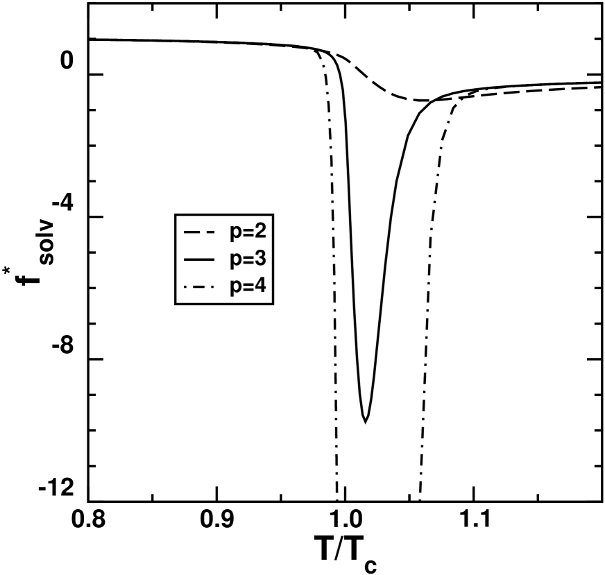
Figure 3: Solvation force for the Ising strip of width $L=100$, $h_{1}\approx 8.16$ rescaled with its value at $T/T_{c}=0.75$, plotted as a function of the reduced temperature. Below $T_{c}$, the results calculated for three different values of the power $p$ lie on a common curve $\sim m^{*}(T/T_{c})$, where $m^{*}(T)$ is bulk spontaneous magnetization. This behaviour agrees with the prediction Eq. (5) with $2\rho B$ replaced by $2m^{*}(T)h_{1}$.

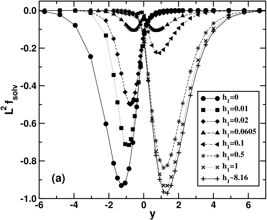
Figure 4: Solvation force (in units of $J$) for the same system as in Fig. 3 as a function of the variable $y$ for a selection of values of the strength parameter $h_{1}$ and for two values of the parameter $p$: (a) $p=50$ and (b) $p=2$. Results for different values of $h_{1}$ in Fig. 4b are represented by the same symbols as in Fig. 4a. It is seen that the symmetry, Eq. (12) between $f_{solv}(y)$ for the free ($h_{1}=0$) and $(++)$ ($h_{1}\sim 8.16$) boundary conditions breaks when the boundary fields become long ranged. For weak $h_{1}$ the solvation force exhibit two minima.

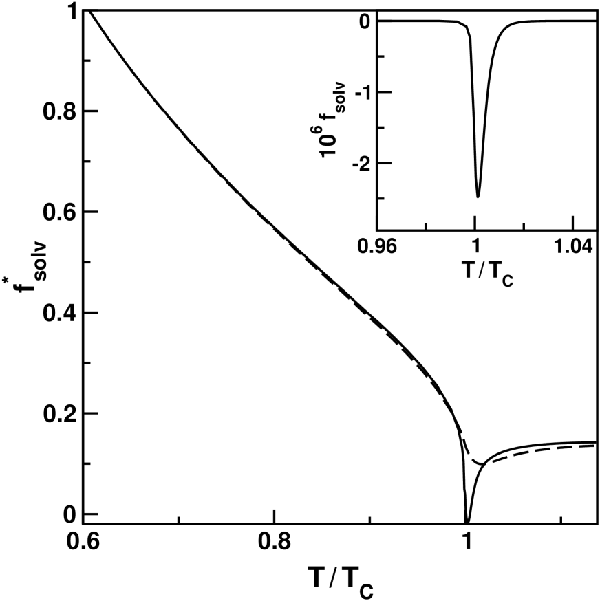
Figure 6: Solvation force rescaled with its value at $T/T_{c}=0.615$, $f_{solv}^{\ast}\equiv f_{solv}(T/T_{c})/f_{solv}(0.615)$, as a function of the temperature for systems with long ranged fluid-wall potentials for $L=50.4\sigma$ evaluated from density functional theory. The chemical potential $\mu(T)$ is chosen so that the reservoir density bulk density $\rho_{b}^{\ast}(T)$ is close to that of the bulk coexisting liquid for $T<T_{c}$ and $\rho_{b}(\mu,T)=\rho_{c}$ for $T\geq T_{c}$. Solid line corresponds to the system with $p=3$, while dashed line is for the system with $p=2$. The inset shows the temperature dependence of $f_{solv}$ for the system with fluid-wall interactions of the finite range.

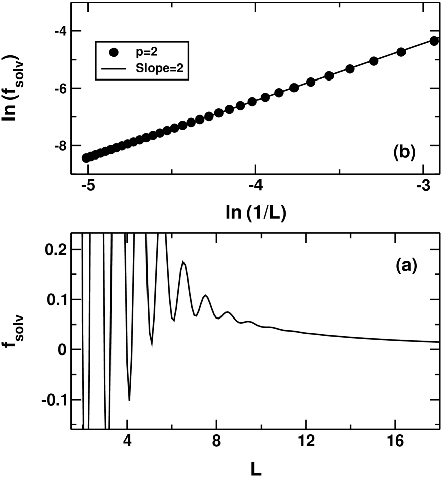
Figure 8: The oscillatory (part a) and asymptotic shown on a $\log-\log$ plot (part b) regions of the solvation force for the system with $p=2$ evaluated from density functional theory. The temperature ($T^{\ast}=1.0$) and the reservoir density ($\rho_{b}^{\ast}=0.6148$) are fixed such that the fluid is just slightly off the coexistence on the liquid branch of the coexistence curve. Note that for $p=2$ the solvation force has more pronounced oscillations than for $p=3$.

Figure 9: Schematic plot of the solvation force for systems with short ranged (part a) and long ranged (part b) fluid-wall interactions in the presence of capillary condensation. Dots denoted by $Z,M$ and $I$ in part b mark characteristic points of the solvation force: the zero, the maximum and the inflection point, respectively.

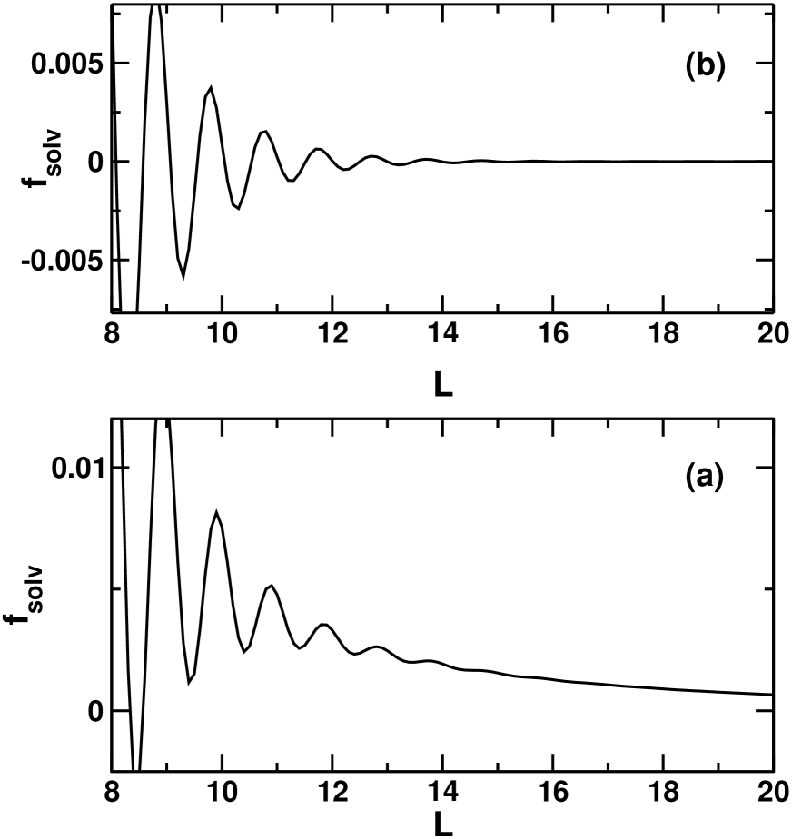
Figure 11: Solvation force for the LJ fluid with the short ranged and long ranged wall-fluid potentials calculated within DFT for $T^{\ast}=1.0$ and $\rho^{\ast}_{b}=0.6853$, the same state point as in the simulations by Pertsin and Grunze pertsin:03:0 . (a) is for the full 9-3 LJ potential. Oscillations characteristic for short wall-wall separations are gradually damped and changed into the power law asymptotic decay. (b) is for the truncated 9-4 LJ potential with the cut-off distance 2.5$\sigma$. Oscillations around 0 are present for all wall-wall separations.

References

- (1) R. Evans, J.Phys.:Condens.Matter. 2, 8989 (1990) and references therein.
- (2) J.N Israelachvili, Intermolecular and Surface Forces (Academic, London, 1991), 2nd ed.
- (3) J.N Israelachvili and G.E. Adams, JCS Faraday Trans. I 74, 975 (1978); J.N Israelachvili, Accounts Chem. Res. 20, 415 (1987).
- (4) C.P. Smith, M. Maeda, L. Atanasoska, H.S. White, and D.J. McClure, J. Phys. Chem. 92, 199 (1988).
- (5) J.L. Parker and H.K. Christenson, J. Chem. Phys. 88, 8013 (1988).
- (6) C.S. Lee and G. Belfort, Proc. Natl. Acad. Sci USA 86, 8392 (1989).
- (7) See, e.g., R. Evans, in Liquids at Interfaces, Les Houches Session XLVIII, edited by J. Charvolin, J. Joanny, and J. Zinn-Justin (Elsevier, Amsterdam, 1990), p. 3.
- (8) R. Evans, D.C. Hoyle, and A.O. Parry, Phys. Rev. A 45, 3823 (1992).
- (9) J.R. Henderson and Z.A. Sabeur, J. Chem. Phys. 97, 6750 (1992).
- (10) R. Evans, J.R. Henderson, D.C. Hoyle, A.O. Parry, and Z.A. Sabeur, Molec. Phys. 80, 755 (1993).
- (11) R. Evans, R.J.F. Leote de Carvalho, J.R. Henderson, and D.C. Hoyle, J. Chem. Phys. 100, 591, (1994).
- (12) R. Evans, U. Marini Bettolo Marconi, and P. Tarazona, J. Chem. Phys. 84, 2376 (1986).
- (13) R. Evans and U. Marini Bettolo Marconi, J. Chem. Phys. 86, 7138 (1987).
- (14) U. Marini Bettolo Marconi, Phys. Rev. A 38, 6267 (1988).
- (15) A.O. Parry and R. Evans, Physica A 181, 250 (1992).
- (16) M. Krech, Phys. Rev. A 56, 1642 (1997).
- (17) A. Hanke, F. Schlesener, E. Eisenriegler, and S. Dietrich, Phys. Rev. Lett. 81, 1885 (1998).
- (18) Z. Borjan and P. Upton (unpublished); Z. Borjan, Ph.D. thesis, University of Bristol, 1999 (unpublished).
- (19) R. Evans and J. Stecki, Phys. Rev. B 49, 8842 (1993).
- (20) M. E. Fisher and P.G. de Gennes, C. R. Acad Sci. Ser. B 287, 207 (1978).
- (21) for review see for example Finite-Size Scaling and Numerical Simulations of Statistical Systems, edited by V. Privman (World Scientific, Singapore, 1990).
- (22) H. Au-Yang and M.E. Fisher, Phys. Rev. B 11,3469 (1975); H. Au-Yang and M.E. Fisher, Phys. Rev. B. 21,3956 (1980).
- (23) D.B. Abraham, Stud. Appl. Math. 50, 71 (1971).
- (24) D.B. Abraham and A. Martin-Löf, Commun. Math. Phys. 32, 245 (1973).
- (25) A. Maciołek, J. Phys. A 39, 3837 (1996); A. Maciołek and J. Stecki, Phys. Rev. B 54, 1128 (1996).
- (26) A. Maciołek, A. Drzewiński, and A. Ciach, Phys. Rev. E 60, 5009 (1999).
- (27) T. Nishino, J. Phys. Soc. Jpn. 64, 3598 (1995).
- (28) E. Carlon and A. Drzewiński, Phys. Rev. Lett. 79, 1591 (1997).
- (29) A. Maciołek, A. Drzewiński, and R. Evans, Phys. Rev. E 64, 056137 (2001).
- (30) P. Attard, D.R. Bérard, C.P. Ursenbach, and G.N. Patey, Phys. Rev. A 44, 8224 (1991).
- (31) M. Krech, The Casimir Effect in Critical System (World Scientific, Singapore, 1994); J. Phys. Condens. Matter 11, R391 (1999).
- (32) A. Maciołek, A. Drzewiński, and R. Evans, Phys. Rev. E 64, 056137 (2001).
- (33) M.E. Fisher and H. Nakanishi, J. Chem. Phys. 75, 5857 (1981); H. Nakanishi and M.E. Fisher, J. Chem. Phys. 78, 3279 (1983).
- (34) F. Schlesener, A. Hanke, and S. Dietrich, J. Stat. Phys. 110, 981 ( 2003).
- (35) S.R. White, Phys. Rev. Lett. 69, 2863 (1992); S.R. White, Phys. Rev. B 48, 10345 (1993).
- (36) Lectures Notes in Physics. V.528 ed. by I. Peschel, X. Wang, M.Kaulke and K. Hallberg (Springer, Berlin 1999).
- (37) A. Drzewiński, A. Ciach, and A. Maciołek, Eur. Phys. J. B 5, 825 (1998).
- (38) G.H. Golub and C.F. Van Loan, Matrix Computations (Baltimore, 1996).
- (39) L. Onsager, Phys. Rev. 65, 117 (1944).
- (40) H.W. Diehl, in Phase Transitions and Critical Phenomena. V. 10 p. 75 ed. by C. Domb and J.L. Lebowitz (Academic Press Inc., London, 1986).
- (41) D. Dantchev, M. Krech, and S. Dietrich, Phys. Rev. E 67, 066120 (2003).
- (42) H. W. Blöte, J. L. Cardy, and M. P. Nightingale, Phys. Rev. Lett. 56, 742 (1986).
- (43) J.D. Weeks, D. Chandler, and H.C. Andersen, J. Chem. Phys. 54, 5237 (1979).
- (44) R. Evans, in Fundamentals of Inhomogeneous Fluids, edited by D. Henderson, (Marcel, New York, 1992).
- (45) Y. Rosenfeld, Phys. Rev. Lett. 63, 980 (1989).
- (46) Y. Rosenfeld, J. Chem. Phys. 98, 8126 (1993).
- (47) J.R. Henderson, in Fundamentals of Inhomogeneous Fluids, edited by D. Henderson, (Marcel, New York, 1992).
- (48) M. Dijkstra and R. Evans, J. Chem. Phys. 98, 8126 (1993).
- (49) R. Evans, Ber. Bunsenges. Phys. Chem. 112, 1449 (2000).
- (50) I. S. Gradshteyn and I. M. Ryzhik, Table of Integrals, Series, and Products, (Academic Press, New York, 1965).
- (51) Keeping all contribution in the Eq. (4) can lead to the result that the total solvation force is always attractive attard:91:0 .
- (52) A.J. Pertsin and M. Grunze, J. Chem. Phys. 118, 8004 (2003).