Dynamics of the spin-boson model with a structured environment

Abstract

We investigate the dynamics of the spin-boson model when the spectral density of the boson bath shows a resonance at a characteristic frequency $\Omega$ but behaves Ohmically at small frequencies. The time evolution of an initial state is determined by making use of the mapping onto a system composed of a quantum mechanical two-state system (TSS) which is coupled to a harmonic oscillator (HO) with frequency $\Omega$. The HO itself is coupled to an Ohmic environment. The dynamics is calculated by employing the numerically exact quasiadiabatic path-integral propagator technique. We find significant new properties compared to the Ohmic spin-boson model. By reducing the TSS-HO system in the dressed states picture to a three-level system for the special case at resonance, we calculate the dephasing rates for the TSS analytically. Finally, we apply our model to experimentally realized superconducting flux qubits coupled to an underdamped dc-SQUID detector.

1 Introduction

The spin-boson model is one of the central paradigms in theoretical physics [1, 2]. The quantum mechanical two-state system (spin 1/2 or in today’s modern language qubit) interacting with a bosonic bath, is the simplest possible model to describe the effect of an environment on constructive and destructive quantum interference. It allows in a rather comprehensive way to investigate decoherence and damping on the quantum system imposed by a phenomenological environment. Hence, it has found numerous applications ranging from electron transfer to quantum information processing.

The characteristics of the harmonic bath in contact with the two-state system is captured by the spectral density $J(\omega)$ of the bath. A well studied special case is the spin-boson model with an Ohmic spectral density, where $J(\omega)\propto\omega$ (up to some cut-off frequency). This implies that the quantum system is damped equally at all frequencies, which is the case for many physical systems. A prominent example in the field of condensed matter physics are single-charge effects in micro- and nanostructured systems in which the electromagnetic environment can be modeled by an impedance of pure Ohmic form. The more general case of $J(\omega)$ having a power-law distribution, i.e., $J(\omega)\propto\omega^{s}$ ($0<s<1$ sub-Ohmic and $s>1$ super-Ohmic bath) also finds wide-spread applications, for instance when the TSS couples to an electromagnetic environment represented by a RC-transmission line. For these specifications, the time constants with which a quantum superposition of the TSS decays can be calculated in analytic form by using real-time path integral techniques [1, 2].
Another limit to be mentioned in this context is the case of a single environmental mode at a specific frequency $\Omega$, i.e., $J(\omega)\propto\delta(\omega-\Omega)$, which is for instance realized by an electromagnetic environment with a pure inductive impedance.

In this work, we consider the spin-boson model for the case of the bath spectral density having a distinct resonance at a characteristic frequency $\Omega$ of the order of the TSS level splitting, and behaving Ohmically a low frequencies (peaked spectral density with Ohmic background). This model currently receives growing interest in the context of quantum computing with condensed matter systems [3], especially for superconducting flux qubit devices [4, 5, 6, 7]. In these devices, the state of the TSS, i.e., the direction of the magnetic flux, is read out by a dc-SQUID which couples inductively to the qubit superconducting loop. At bias currents well below the critical current $I_{C}$, the SQUID can be modeled as an inductor $L_{J}$. An additional shunt capacitance $C_{s}$ creates an on-chip environment which improves the resolution of the dc-SQUID. The resulting impedance of this dc-SQUID environment can display a pronounced resonance at the characteristic frequency of the $LC$-circuit (see below for details).
As an alternative but equivalent point of view, a TSS coupled to a harmonic bath with a peaked spectral density represents an effective description of a TSS coupled to a damped harmonic oscillator of characteristic frequency $\Omega$. In this perspective, this model has recently been used to describe solid state implementations of a qubit coupled to a resonator. Various schemes of measurement, entanglement generation, quantum information transfer and interaction with a nonclassical state of the electromagnetic field have been proposed [8, 9] and dephasing effects have been addressed [9]. Moreover these devices, besides being promising candidates for realizing qubits in a possibly scalable quantum computer, are also very interesting objects to display fundamental quantum physical properties, like macroscopic quantum coherence [10], Rabi oscillations [6, 11, 12], Ramsey interference [6, 13], etc.

The spin-boson model with a peaked spectral density of the bath has been investigated theoretically in Refs. [14, 15]. In Ref. [14], it has been demonstrated that an external driving field can be applied to slow down decoherence by moving the TSS out of resonance with the HO due to dressing of the TSS by the driving field. Recently, Kleff et al. [15] have calculated for the static case at zero temperature dephasing times by applying the numerical flow equation renormalization method (see below for further remarks).

To explore the more realistic finite-temperature dynamics of the spin-boson model with a resonance peak at frequency $\Omega$ in the spectral density of the bath, we make use of the already mentioned exact mapping to a TSS+HO model [16]. By this, we obtain a model consisting of the TSS which couples to a harmonic oscillator with characteristic frequency $\Omega$, which itself couples to a harmonic bath with Ohmic spectral density. Throughout this work, we concentrate on the case of a weak coupling of the oscillator to the Ohmic bath, but the TSS-HO coupling is kept arbitrary. This choice of the parameter region is due to the experimentally given situation of dc-SQUIDs which are typically underdamped. This mapping allows to apply the numerically exact method of the quasi-adiabatic propagator path-integral (QUAPI) [17] for the TSS+HO being the the central quantum system. Ay additionally tracing out the HO degrees of freedom, we determine the time-evolution of the reduced density matrix of the TSS. We extract the dephasing and relaxation time constants for the decay of a localized state of the TSS. In order to elaborate the difference, we compare our numerical results to the well-known analytical expressions for the rates of a TSS coupled to a structured harmonic reservoir evaluated to lowest order in the TSS-reservoir coupling [18]. As it turns out, these weak-coupling rates deviate considerably (up to a factor of 50) from the numerically exact decay rates for level splittings around the oscillator frequency. This shows that if the frequencies of the TSS and the HO are comparable, the decay rates are determined by the full frequency spectrum of the peaked environment, and not only by its low frequency weak Ohmic backround. Next, we concentrate on the specific case of the TSS being exactly in resonance with the oscillator and establish a simple three-level description of the TSS-HO system. Since we are interested in weak system-bath coupling, we formulate the Redfield equations for this three-level system (3LS) which can be solved analytically. The resulting dephasing rates agree well with the numerically exact values of QUAPI. Finally, we apply our general model to experimentally realized superconducting flux qubit devices.

2 The model and the mapping to a TSS+HO Hamiltonian

To setup the model, we consider the Hamiltonian of a two-state system being coupled to a bath of (non-interacting) harmonic oscillators, i.e.,

$$\tilde{H} = -\frac{\hbar\Delta_{0}}{2}\sigma_{x}-\frac{\hbar\varepsilon}{2}\sigma_{z}+\frac{1}{2}\sigma_{z}\hbar\sum_{k}\tilde{\lambda}_{k}(\tilde{b}_{k}^{\dagger}+\tilde{b}_{k})+\sum_{k}\hbar\tilde{\omega}_{k}\tilde{b}_{k}^{\dagger}\tilde{b}_{k}\,.$$ (1)

Here, $\tilde{b}_{k}$ and $\tilde{b}_{k}^{\dagger}$ are the annihilation and creation operators of the $k-$th bath mode with frequency $\tilde{\omega}_{k}$. The spectral density of the bath modes is assumed to have a Lorentzian peak at the characteristic frequency $\Omega$, but behaves Ohmically at low frequencies with the dimensionless coupling strength $\alpha=\lim_{\omega\rightarrow 0}J(\omega)/2\omega$. The Lorentzian-shaped resonance has a width which we denote as $\gamma=2\pi\kappa\Omega$. To be specific, we assume a spectral density of the form

$$J(\omega) = \sum_{k}\tilde{\lambda}_{k}^{2}\delta(\omega-\tilde{\omega}_{k})=\frac{2\alpha\omega\Omega^{4}}{(\Omega^{2}-\omega^{2})^{2}+(2\pi\kappa\omega\Omega)^{2}}\mbox{\hskip 8.61108pt}\stackrel{{\scriptstyle\omega\rightarrow 0}}{{\longrightarrow}}2\alpha\omega\,.$$ (2)

For our purposes, it is convenient to aquire a different viewpoint as it will become clear below. Following Ref. [16, 14], there exists an exact one-to-one mapping of this Hamiltonian onto that one of a TSS coupled to a single HO mode with frequency $\Omega$ which itself interacts with a set of (non-interacting) harmonic oscillators having an Ohmic spectral density with the dimensionless damping strength $\kappa$. Thereby, the interaction strength between the TSS and the HO is given by $g$. The corresponding Hamiltonian reads

$$H = -\frac{\hbar\Delta_{0}}{2}\sigma_{x}-\frac{\hbar\varepsilon}{2}\sigma_{z}+\hbar g\sigma_{z}(B^{\dagger}+B)+\hbar\Omega B^{\dagger}B$$ (3)

$$+(B^{\dagger}+B)\sum_{k}\hbar\nu_{k}(b_{k}^{\dagger}+b_{k})+\sum_{k}\hbar\omega_{k}b_{k}^{\dagger}b_{k}\,.$$

Here, $B$ and $B^{\dagger}$ are the annihilation and creation operators of the localized HO mode while the $b_{k}$ and the $b_{k}^{\dagger}$ are the corresponding bath mode operators. The spectral density of the continuous bath modes now becomes Ohmic, i.e.,

$$J_{\rm Ohm}(\omega)=\sum_{k}\nu_{k}^{2}\delta(\omega-\omega_{k})=\kappa\omega e^{-\omega/\omega_{c}}\,,$$ (4)

where we have introduced the usual high-frequency cut-off at $\omega_{c}$ (We note that throughout this work, we use the value $\omega_{c}=10\Delta_{0}$). The relation between $g$ and $\alpha$ follows as

$$g=\Omega\sqrt{\frac{\alpha}{8\kappa}}\hskip 12.91663pt\Leftrightarrow\hskip 12.91663pt\alpha=8\kappa\frac{g^{2}}{\Omega^{2}}\,.$$ (5)

Since for our cases of interest, the damping of the HO is small ($\kappa\ll 1$), we will denote the TSS+HO-system as the central quantum system which is itself weakly damped. However, the coupling between the TSS and the HO can still become large. In the following, we will evaluate the reduced density operator $\rho_{TSS+HO}(t)=tr_{\rm bath}e^{iHt/\hbar}W(0)e^{-iHt/\hbar}$ for the TSS+HO-system, where the bath degrees of freedom have been traced out. $W(0)$ denotes the full density operator at initial time $t=0$. Throughout this work, we assume a factorizing initial preparation where all three parts of the total system are decoupled and the coupling is switched on instantaneously at $t=0^{+}$. In particular, we choose the bath being at thermal equilibrium at inverse temperature $\beta=1/k_{B}T$ as well as the localized mode being thermally distributed. This implies

$$W(0)=\rho_{TSS}(0)\otimes\frac{e^{-\beta H_{HO}}}{Z_{HO}}\otimes\frac{e^{-\beta H_{bath}}}{Z_{bath}}\;,$$ (6)

where $Z$ denotes the partition function of the corresponding subsystem. The further reduction to the reduced density operator $\rho(t)$ of the TSS alone is easily done by tracing out the HO degrees of freedom, i.e., $\rho(t)=tr_{HO}\,\rho_{TSS+HO}(t)$.

3 Observables

Having calculated the reduced density matrix $\rho(t)$ of the TSS, we can directly calculate the observables of interest. In this context, we are interested in the dephasing and relaxation rates of the TSS dynamics. Hence, we prepare the TSS in a symmetric superposition of its energy eigenstates. The relevant dynamical quantity then is the symmetrized correlation function

$$S_{z}(t)=\frac{1}{2}\langle\sigma_{z}(t)\sigma_{z}(0)+\sigma_{z}(0)\sigma_{z}(t)\rangle-\langle\sigma_{z}\rangle^{2}_{\infty,+}\,,$$ (7)

where $\sigma_{z}(t)=e^{iHt/\hbar}\sigma_{z}e^{-iHt/\hbar}$ and where the equilibrium population $\langle\sigma_{z}\rangle^{2}_{\infty,+}$ (the subscript $+$ indicates that the dynamics has been calculated with positive bias $\varepsilon>0$) has been subtracted. By assuming a factorizing initial preparation, the correlation function can be expressed in terms of the population difference $P_{+}(t)\equiv\langle\sigma_{z}\rangle_{t}=P_{s}(t)+P_{a}(t)$. It follows

$$S_{z}(t)=P_{s}(t)+P_{\infty,+}[P_{a}(t)-P_{\infty,+}]\,,$$ (8)

where $P_{s/a}(t)$ are the symmetric/antisymmetric parts of $P_{+}(t)$ with respect to the sign of the bias and $P_{\infty,+}\equiv\langle\sigma_{z}\rangle^{2}_{\infty,+}$. This quantity vanishes at long times which ensures that the Fourier transform exists. By calculating the population $P_{-}(t)$ with the sign of the bias inverted ($\varepsilon<0$), we obtain $P_{s/a}(t)$ according to

$$P_{s}(t) = [P_{+}(t)+P_{-}(t)]/2\,,$$

$$P_{a}(t) = [P_{+}(t)-P_{-}(t)]/2\,.$$ (9)

For the unbiased case $\varepsilon=0$, we have $S_{z}(t)=P_{s}(t)\equiv P(t)$. Moreover, the initial preparation $\rho_{TSS}(0)$ of the TSS in an equally weighted superposition of ground and excited state implies $P_{+}(0)=P_{-}(0)=1$. Since $S_{z}(t)$ vanishes at $t\rightarrow\infty$, it readily can be Fourier transformed, i.e.,

$$S_{z}(\omega)=2\int_{0}^{\infty}dt\cos\omega t\,S_{z}(t)\,.$$ (10)

To extract the decay rates $\Gamma_{i}$, the frequencies $\omega_{i}$ and the spectral weights $a_{i}$ associated to $S_{z}(\omega)$, we approximate $S_{z}(t)$ as a sum of exponentially decaying sinusoids, i.e.,

$$S_{z}(t)=\sum_{i}a_{i}e^{-\Gamma_{i}t}\cos{\omega_{i}t}\,,$$ (11)

where $\sum_{i}a_{i}=1$. It has the Fourier transform

$$S_{z}(\omega)=\sum_{i}a_{i}\left[\frac{\Gamma_{i}}{\Gamma_{i}^{2}+(\omega_{i}+\omega)^{2}}+\frac{\Gamma_{i}}{\Gamma_{i}^{2}+(\omega_{i}-\omega)^{2}}\right]\;.$$ (12)

By a standard fitting procedure, we fit the exact numerical results to this function to extract the decay rates $\Gamma_{i}$ (HWHM of the Lorentzian peak), the frequencies $\omega_{i}$ (position of the peak) and the spectral weights $a_{i}$.

4 The numerical ab-initio technique QUAPI

In order to calculate the reduced density operator, we use the iterative tensor multiplication scheme derived for the so-called quasiadiabatic propagator path integral (QUAPI). This numerical algorithm was developed by Makri and Makarov [17] within the context of chemical physics. Since its first applications it has been successfully tested and adopted to various problems of open quantum systems, with and without external driving [17, 19, 20, 21]. The details of this technique have been discussed to a great extent in the literature [17, 19, 20, 21] and we only mention briefly how to adopt it to our specific problem.

We use QUAPI to calculate the reduced density matrix $\rho(t)$ and iterate until the stationary state of $P_{\pm}(t)$ has been reached. For the biased case, we run the iteration with both positive and negative bias to calculate $P_{\pm}(t)$ ($\varepsilon>0$ and $\varepsilon<0$). Having transformed to $P_{s/a}(t)$, see Eq.  (9), we determine $S_{z}(t)$ in Eq.  (8) and Fourier transform the result to determine $S_{z}(\omega)$ according to Eqs.  (10,). Then, a fit to Eq.  (12) determines the dephasing and relaxation rates $\Gamma_{i}$ (HWHM of the Lorentzian peak), the frequencies $\omega_{i}$ (position of the peak) and the spectral weights $a_{i}$. A typical result for the symmetric TSS ($\varepsilon=0$) being in resonance with the HO ($\Delta_{0}=\Omega$) is shown in Fig.  1, see also Section 9.2 for a more detailed discussion of this specific case. The inset of Fig.  1 depicts the time evolution of $P(t)$. The Fourier transform displays two characteristic peaks at $\omega=\omega_{1}$ and $\omega=\omega_{2}$. The width of these peaks can be read of the fitted Lorentzians, see dashed lines.

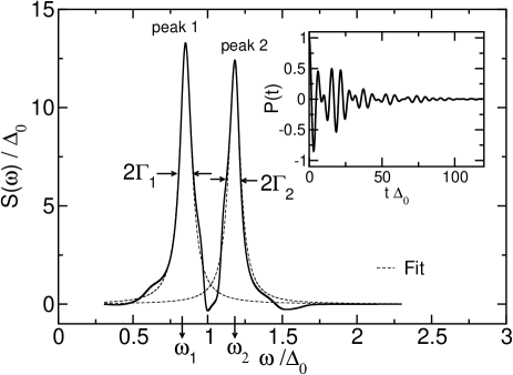
Figure 1: Example of the dynamics for the symmetric case $\varepsilon=0$, where the oscillator frequency is in resonance with the TSS frequency, i.e., $\Omega=\Delta_{0}$. Parameters are: $g=0.18\Delta_{0}$, $\kappa=0.014(\rightarrow\alpha=0.004),k_{B}T=0.1\hbar\Delta_{0}$. QUAPI parameters are $M=12,K=1,\Delta t=0.06/\Delta_{0}$.

QUAPI uses three free parameters which have to be adjusted according to the particular situation. Typical physically reasonable situations allow for a tractable choice of parameters.
(i) The first parameter is the dimension $M$ of the Hilbert space of the quantum system which is in our case the composed TSS+HO-system. With the dimension of the TSS being fixed, we truncate the in principal infinite dimensional oscillator basis to the six lowest energy eigenstates leading to $M=12$. We have checked convergence also with $M=16$ and $M=20$ and found the results unchanged.
(ii) The second parameter affects the length of the memory which is induced by the environmental correlations. This memory time has the length of $K$ times the time step of the iteration. Here, we deal with weak Ohmic damping ($\kappa\ll 1$) of the HO and temperature in the experimental devices is typically larger than damping. (This in principle would even allow for a Markovian approximation.) In our case, this permits to choose $K$ small. We fix $K=1$. We have also ensured convergence by choosing $K=2$, but the results changed only by less than 10 %. This is depicted in Fig.  2. The results for peak 1 are for $K=1:\Gamma_{1}=0.0177,\omega_{1}=0.730,a_{1}=0.197$ (in units of $\Delta_{0}$) while for $K=2:\Gamma_{1}=0.0166,\omega_{1}=0.718,a_{1}=0.181$. For peak 2, we find the values $K=1:\Gamma_{2}=0.0310,\omega_{2}=1.074,a_{2}=0.913$, while for $K=2:\Gamma_{2}=0.0282,\omega_{2}=1.073,a_{2}=0.917$. The sum rule $a_{1}+a_{2}=1$ is fulfilled with an accuracy of approximately $10{\%}$.

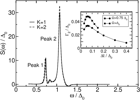
Figure 2: Main: Fourier transform $S_{z}(\omega)$ for two different memory lengths $K=1$ and $K=2$, see text. Parameters: $\varepsilon=0,g=0.18\Delta_{0}$, $\Omega=0.75\Delta_{0},\kappa=0.014(\rightarrow\alpha=0.006),k_{B}T=0.1\hbar\Delta_{0}$. Remaining QUAPI parameters are $M=12,\Delta t=0.06/\Delta_{0}$. Inset: Dephasing rate $\Gamma_{2}$ for different QUAPI-time steps $\Delta t$ for two different values of $\Omega$. The position of the maxima determine the choice of $\Delta t$ for QUAPI, see text.

At this point, it becomes clear why it is essential for QUAPI to use the mapping to the TSS+HO model. For the dynamics of the spin-boson model with the peaked spectral density in Eq. (2), the autocorrelation function $L(t)=\langle\xi(t)\xi(0)\rangle,t>0$, of the fluctuating force $\xi(t)$ of the bath [1] decays slowly with time in an oscillatory way. This can be readily understood since $L(t)$ is qualitatively the Fourier transform of $J(\omega)$. In other words, the peaked environment possesses a longer correlation time compared to the Ohmic bath. This is also the reason why a standard weak-coupling approach fails to determine the dephasing rates (see Sec. 9.1 for a detailed comparison between both approaches). Since the long correlation time of the peaked bath would require a long memory time $K\Delta t$ with $K\gg 1$, the direct treatment of the TSS coupled to the peaked bath with QUAPI is still beyond the today’s computational resources. Only the corresponding Ohmic autocorrelation function decays fast enough with time to be truncated after a relatively short memory time (at any finite temperature $T$). It is computationally more favorable to iterate the HO dynamics as a part of the quantum system and not as a part of the bath.
We mention that for the comparison with the three-level approximation (see Section 9.2 below), which is expected to be good at low temperatures, we used the parameters $M=6$ and $K=3$, since in this case the bath-induced correlations have a weaker decay and hence require a longer memory time. Also, the lower temperature allows to restrict to less basis states.
(iii) The third QUAPI-parameter is the time-step $\Delta t$. It is fixed according to the principle of minimal sensitivity [20] of the result on the variation of $\Delta t$. The results which permits to decide on $\Delta t$ are shown in the inset of Fig. (2). The position of the maxima determine the choice of $\Delta t$. In our case, we fix $\Delta t=0.06/\Delta_{0}$. As one can observe from Fig. (2), the position of the maximum is not sensitive on the change of the parameter $\Omega$.

5 Varying the oscillator frequency $\Omega$

In this section, we investigate the effect of varying the frequency $\Omega$ of the resonance of the spectral density $J(\omega)$ in Eq. (2), or, in other words, the frequency of the harmonic oscillator. For simplicity, we restrict here to the symmetric TSS $\varepsilon=0$. For the biased TSS, the qualitative behavior is similar if one replaces $\Delta_{0}$ by the effective level splitting $\Delta_{b}=\sqrt{\Delta_{0}^{2}+\varepsilon^{2}}$ for the biased case.

5.1 Exact resonance $\Omega=\Delta_{0}$

The dynamics of the TSS being in resonance with the HO is depicted in Fig. 1 for a typical set of parameters (see caption). One observes a decay of $P(t)$ with two frequencies and two damping constants. This can be readily understood by considering the undamped TSS+HO-system, i.e., $\kappa=0$. To diagonalize the corresponding Hamiltonian, we can use the rotating-wave approximation (RWA), which is appropriate at resonance. Treating the interaction $g$ in first order perturbation theory, we obtain the spectrum as a ladder of energy-levels. The groundstate $|g,0\rangle$ ($g$ denotes the groundstate of the TSS while $0$ denotes the index of the HO mode) is separated by $n\hbar\Omega$ from the higher lying n-th pair of excited states which are almost degenerate, but split by $\hbar\overline{\Delta}_{n}=2\hbar g\sqrt{n}$. At rather low temperature, only the three lowest energy eigenstates, i.e., the ground state $|g,0\rangle$ and the first ($n=1$) pair of excited states are relevant. This yields to two peaks in the spectrum at $\omega_{1}=\Delta_{0}-g$ and at $\omega_{2}=\Delta_{0}+g$ with the distance $\Delta_{1}=2g$ which appears in Fig.  1. The two peaks have almost the same height, i.e., the same spectral weight $a_{1}\approx a_{2}$.

5.2 Negative detuning $\Omega<\Delta_{0}$

If the HO frequency is detuned from the TSS level splitting such that $\Omega<\Delta_{0}$, the dynamics of $P(t)$ also contains two frequencies but with different spectral weights. This is shown in Fig. 3 for $\Omega=0.75\Delta_{0}$. Also, a perturbative analysis of second order in $g$ (the first order vanishes exactly), readily explains the features: again restricting to the three lowest energy eigenstates, we find that the first excited state $|g,1\rangle$ is separated from the ground state $|g,0\rangle$ by $\omega_{1}=\Omega-\frac{2g^{2}\Delta_{0}}{\Delta_{0}^{2}-\Omega^{2}}\approx\Omega-\frac{g^{2}}{\Delta_{0}-\Omega}$, where in the last relation the RWA has been used. The almost degenerate next higher lying excited state $|e,0\rangle$ is separated from the ground state by $\omega_{2}=\Delta_{0}+\frac{2g^{2}\Delta_{0}}{\Delta_{0}^{2}-\Omega^{2}}\approx\Delta_{0}+\frac{g^{2}}{\Delta_{0}-\Omega}$. These two frequencies show up in the spectrum, see Fig. 3. The perturbatively calculated values of the peak positions are for these parameters $\omega_{1}=0.73\Delta_{0}$ and $\omega_{1}=1.02\Delta_{0}$. The spectral weights of the peaks are different, i.e., $a_{1}\ll a_{2}$.

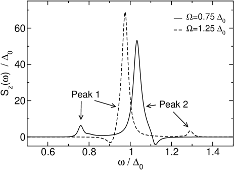
Figure 3: $S_{z}(\omega)$ for two values of the oscillator frequency $\Omega$. Parameters are: $\varepsilon=0,g=0.07\Delta_{0}$, $\kappa=0.014,k_{B}T=0.1\hbar\Delta_{0}$.

5.3 Positive detuning $\Omega>\Delta_{0}$

For the case of positive detuning $\Omega>\Delta_{0}$, also two frequencies appear, see Fig.  3. A perturbative treatment as in Subsection 5.2 gives the frequency of the peaks at $\omega_{1}=\Delta_{0}+\frac{2g^{2}\Delta_{0}}{\Delta_{0}^{2}-\Omega^{2}}\approx\Delta_{0}+\frac{g^{2}}{\Delta_{0}-\Omega}$ and $\omega_{2}=\Omega-\frac{2g^{2}\Delta_{0}}{\Delta_{0}^{2}-\Omega^{2}}\approx\Omega-\frac{g^{2}}{\Delta_{0}-\Omega}$, where in the last relations the RWA has been used again. For the parameters used in Fig. 3, the results are $\omega_{1}=0.98$ and $\omega_{2}=1.27$ which agree well with the positions of the peaks in the spectrum. The spectral weights are in this case inverted, i.e., $a_{1}\gg a_{2}$.

5.4 Dephasing rates

In order to extract the dephasing rates $\Gamma_{i}$, we fit two Lorentzians to the peaks in the spectrum shown in Figs.  1 and 3. The dephasing rates follow according to Eq. (12). The dependence of the dephasing on the frequency of the HO is shown in Fig.  4. The main figure displays the result if the interaction strength $g$ between TSS and HO is kept fix, while its inset depicts the result for $\alpha$ kept fix, i.e., $g$ also varies with varying $\Omega$. Each figure displays the dephasing rates of both peaks. The dominating peak with the dominant spectral weight is peak 2 for negative detuning $\Omega<\Delta_{0}$, while it is peak 1 for positive detuning $\Omega>\Delta_{0}$. Both peaks show a clear maximum at which the dephasing is largest. This happens naturally in the vicinity of the resonance $\Omega\approx\Delta_{0}$, where the effect of the coupling of the TSS to the HO is most effective and therefore dephasing of the HO penetrates through to the TSS best.
The inset of Fig.  4 can be readily compared to the result of the recent work by Kleff et al., see Fig. 3b of Ref. [15]. There, the dephasing rate shows a particular almost discontinuous dependence on the ratio of $\Omega/\Delta_{0}$ around 1. In contrast to their findings, we do not observe such a type of behavior but instead a rather smooth dependence. The almost discontinuous feature is likely to be due to the fact that in Ref. [15], the zero temperature dynamics has been considered.

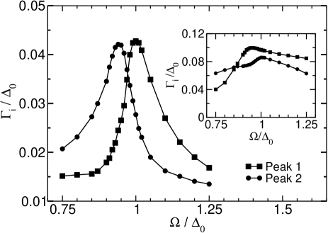
Figure 4: Main: Dephasing rates corresponding to peak 1 and peak 2 in the Figs.  1 and 3 as a function of the HO frequency $\Omega$. The parameters are: $\varepsilon=0,g=0.07\Delta_{0}$, $\kappa=0.014,k_{B}T=0.1\hbar\Delta_{0}$. Inset: Same for stronger damping $\kappa=0.02$ with $\alpha=0.01=$const. (like in Ref. [15]). This implies that with varying $\Omega$ also $g$ is changed.

6 Varying the TSS-HO coupling strength $g$

The dependence of the dephasing rates on the coupling $g$ between the TSS and the HO is depicted in Fig. 5 for the case of negative detuning $\Omega<\Delta_{0}$. As expected, it increases monotonically with increasing $g$ and for this case, peak 2 is dominating, see the spectral weights $a_{i}$ in the inset of Fig. 5. When the coupling $g$ between the TSS and the decoherent HO is increased, dephasing of the TSS is also larger. In general, the dependence of the dephasing on $g$ is observed to be rather weak, as long as $g<\Delta_{0}$, which is usually the case.

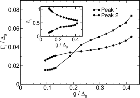
Figure 5: Main: Dephasing rates in dependence of the coupling $g$ between the TSS and the HO for negative detuning $\Omega=0.75\Delta_{0}$. For the remaining parameters see Fig.  4. Inset: The corresponding spectral weights $a_{i}$. One observes that peak 2 is dominating for this detuning.

7 The role of temperature $T$

As in the pure Ohmic spin-boson system for weak damping, we also expect a rather weak dependence of the dephasing rate on temperature in the region of low $T$ for this more complicated system. Indeed, the results confirm this, see Fig.  6. The dephasing rates related to both peaks are almost constant with temperature $T$.

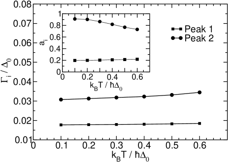
Figure 6: Temperature dependence of the dephasing rates $\Gamma_{1}$ and $\Gamma_{2}$ for the same parameters as in Fig. 4 (main) for $\Omega=0.75$. Inset: Corresponding spectral weights $a_{i}$.

8 Dynamics in presence of a finite bias $\varepsilon\neq 0$

In this section, we consider the case of a biased TSS. Due to this bias, the spectrum shows two more resonances: (i) the relaxation peak at $\omega=0$, (ii) an additional dephasing peak. The frequency of the latter can be estimated by second order perturbation theory in $g$. It corresponds to the energy difference between the states $|e,0\rangle$ and $|g,1\rangle$, which is $\omega_{3}=\Delta_{b}-\Omega+\frac{2g^{2}}{\Delta_{b}-\Omega}$. A typical spectrum is shown in Fig. 7. For this set of parameters, we obtain $\omega_{3}=0.46\Delta_{0}$, which agrees well with the position of the numerically obtained resonance. The remaining two dephasing peaks at $\omega_{1,2}$ correspond to those of the unbiased case with the substitution $\Delta_{0}\rightarrow\Delta_{b}$.

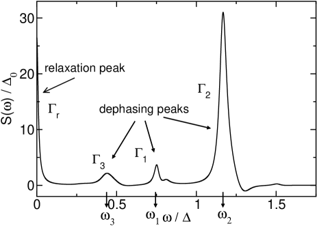
Figure 7: Fourier transform $S_{z}(\omega)$ for the biased case $\varepsilon=0.5$. Compared to the unbiased case, two more resonances appear: the relaxation peak of width $\Gamma_{r}$ at $\omega=0$ and a third dephasing peak of width $\Gamma_{3}$ at $\omega=\omega_{3}$. Parameters are: $\Omega=0.75\Delta_{0},g=0.13\Delta_{0}$, $\kappa=0.014(\rightarrow\alpha=0.003),k_{B}T=0.1\hbar\Delta_{0}$.

The relaxation and the dephasing rates, $\Gamma_{r}$ and $\Gamma_{d_{i}}$, respectively, for increasing bias are shown in Fig.  8. Note that we show only the dephasing rate of the dominant peak 2, i.e., of that one with the largest spectral weight. The qualitative behavior of the rates corresponding to the remaining two dephasing peaks is similar (not shown).

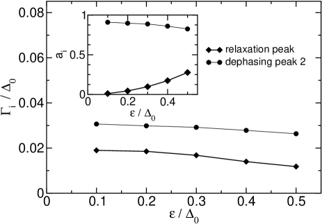
Figure 8: Relaxation rate $\Gamma_{r}$ and dephasing rate $\Gamma_{2}$ for varying bias $\varepsilon$. Only the dominant dephasing peak is considered. The qualitative behavior of the other two rates is similar (not shown). Parameters are: $\Omega=0.75\Delta_{0},g=0.13\Delta_{0}$, $\kappa=0.014(\rightarrow\alpha=0.003),k_{B}T=0.1\hbar\Delta_{0}$. Inset: Corresponding spectral weights $a_{i}$.

As one observes, the decay rates decrease with increasing bias for this case. This can be understood by considering the position of the resonance at $\Omega$ relative to the TSS level spacing $\Delta_{0}$ for zero bias in the spectral density $J(\omega)$, Eq. (2). For the case shown in Fig. 8, $\Omega<\Delta_{0}$. If we increase the bias $\varepsilon$, the effective TSS level spacing $\Delta_{b}$ increases. Since the spectral density is then decreasing (we move on the right flank of the resonance in Eq.  (2) towards larger $\omega$), dephasing is less effective leading to decreasing decay rates. This reasoning can directly be verified by considering the opposite situation $\Omega>\Delta_{0}$ (not shown). In this case, an increasing bias moves the TSS level splitting towards increasing spectral weights, since we are moving on the left flank of the $\Omega$-resonance in Eq. (2), causing an increase of the dephasing and relaxation.

9 Approximate analytical approaches

The standard analytical approach to the reduced dynamics of a TSS weakly coupled to an environment consists in solving a master equation for the reduced density operator [22, 1]. Path-integral methods [1], as well as the Bloch-Redfield formalism can for instance be used [23]. The spin-boson system has been investigated in great detail for the case of weak-coupling to an Ohmic bath, having a continuous spectral density. The most general description dates back to Argyres and Kelly [23] where also strong time-dependent driving has been included. Recently, the equivalence between the the path-integral approach and the Bloch-Redfield theory has been demonstrated in Ref.  [24].

In this section we shall apply a weak coupling approach to our problem, and compare with the exact numerical results presented in the previous sections. In view of the possible application to more complex systems, it is in fact important to understand for this simple problem, in which regime the perturbative estimate differs from the exact solution. In addition, the weak-coupling approach is widely used to estimate the dephasing and relaxation rates in solid-state qubits [4, 6, 25].

In the second part of this section, we will show that a more appropriate approach to the problem of decoherence due to a structured environment consists in enlarging the Hilbert space of the quantum system in order to include the harmonic oscillator.

9.1 Comparison with the spin-boson model for weak damping

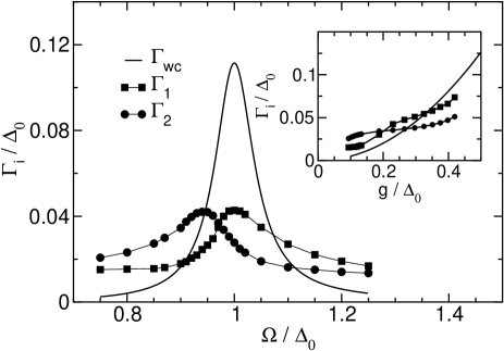
Figure 9: Dephasing rates $\Gamma_{1}$ and $\Gamma_{2}$ in comparison with the weak-coupling rate $\Gamma_{\rm d}$ for varying $\Omega$. Parameters are: $\varepsilon=0,g=0.07\Delta_{0}$, $\kappa=0.014(\rightarrow\alpha=0.0005$ for $\Omega=\Delta_{0}),k_{B}T=0.1\hbar\Delta_{0}$. Inset: Corresponding results for varying $g$ for $\Omega=0.75\Delta_{0}$.

For the spin-boson system the dephasing and relaxation rates can be evaluated analytically to lowest order in the coupling to the bath [1, 18]. For the case of a spectral density showing Ohmic behavior at low frequency, like Eq.(2), they read

$$\Gamma_{d} = \frac{\Gamma_{r}}{2}+\frac{\pi\varepsilon^{2}}{\Delta_{b}^{2}}\frac{2\alpha k_{B}T}{\hbar}$$

$$\Gamma_{r} = \frac{\pi\Delta_{0}^{2}}{2\Delta_{b}^{2}}J(\Delta_{b})\coth\frac{\hbar\Delta_{b}}{2k_{B}T}\,,$$ (13)

where $\Delta_{b}=\sqrt{\Delta_{0}^{2}+\varepsilon^{2}}$. The results for the varying parameters $\Omega,g,T$ are shown in Figs. 9 and 10 for the symmetric case. The dependence on the bias $\varepsilon$ is depicted in the inset of Fig. 10. We show only the results for the dephasing rates, the relaxation rate $\Gamma_{r}$ behaves in a qualitatively similar way.
We notice that the weak-coupling rates Eq.  (13) give a good estimate of the dephasing rate only if $\Omega\gg\Delta_{b}$. This result can be understood considering the physics of the model in the form given in Eq.  (3). If we regard the TSS as coupled to an environment represented by the damped HO, where $g$ is the coupling constant, the rates in Eq.  (13) follow from the usual Bloch-Markov treatment. This latter approach is valid when $g\,\tau_{c}\ll 1$, where $\tau_{c}$ represents the typical correlation times of the weakly damped oscillator [22]. In the temperature regime considered $\tau_{c}$ may be identified with the damping rate of the HO, $\gamma^{-1}$ [1]. Thus, the perturbative approach holds when $g\ll\gamma$. With the parameters of Fig.9, this condition is satisfied for ${\Omega\over\Delta_{0}}\gg 0.8$.

Of course the weak-coupling rates in Eq.  (13) fail in describing the dephasing rates if the TSS is close to or at resonance with the HO. For $\Omega\approx\Delta_{0}$, the weak-coupling rates in Eq. (13) overestimate the dephasing because there are coherent exchange processes between the TSS and the HO mode which are not captured in a weak-coupling approach. It is interesting to notice that for $\Omega<\Delta_{0}$ the damped HO behaves as an environment with long correlation times, and the weak coupling theory fails because of memory effects. The results in Eq.  (13) underestimates the dephasing rate in the regime $\Omega<\Delta_{0}$, a feature which has already been noticed for environments responsible for $1/f$ noise [26].

In fact, a weak-coupling approach is appropriate as long as the correlation time of the bath is sufficiently short (as it is the case for an Ohmic bath with small $\alpha$). However, the presence of the peak in the bath spectral density induces bath correlations which decay only on a time scale given by the width of the resonance.

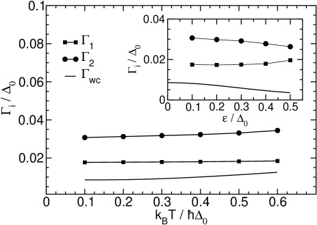
Figure 10: Same as Fig.  9 for varying temperature $T$. Parameters are: $\varepsilon=0,\Omega=0.75\Delta_{0},g=0.13\Delta_{0}$, $\kappa=0.014(\rightarrow\alpha=0.003)$. Inset: Corresponding results for varying the bias $\varepsilon$ for $k_{B}T=0.1\hbar\Delta_{0}$.

9.2 Three-level system as an approximative description

In order to obtain an analytical expression for the dephasing rates, we restrict for simplicity to the simplest case of resonance $\Omega=\Delta_{0}$ between the TSS and the HO. Since the deviation from the pure Ohmic case is most pronounced here, this is also the most interesting case for an analytical solution. We furthermore assume an unbiased TSS, $\varepsilon=0$. All the following considerations can be generalized to the off-resonant case and also with a biased TSS. The expressions, however, will become more involved. As it turns out, the TSS+HO can be restricted at low temperatures to a three-level-system (3LS) having performed second order perturbation theory in $g$. Assuming weak coupling to an Ohmic bath, we can derive the Redfield equations which can be solved analytically. By this, we obtain closed expressions for the dephasing rates $\Gamma_{i}$ and the frequencies $\omega_{i}$.

9.2.1 Redfield equations

To start, we diagonalize the TSS+HO Hamiltonian which corresponds to the substitution $\sigma_{x}\rightarrow\sigma_{z}$ and $\sigma_{z}\rightarrow-\sigma_{x}$ (the resulting transformed operators are denoted by the overline). Moreover, we apply the rotating wave approximation (RWA) which is appropriate at resonance. Together with $\sigma_{x}=\sigma_{+}+\sigma_{-}$, we obtain $\overline{H}^{RWA}_{TSS+HO}=-\frac{\hbar\Delta_{0}}{2}\sigma_{z}+\hbar\Omega B^{\dagger}B-\hbar g(B\sigma_{+}+B^{\dagger}\sigma_{-})$. This is the Jaynes-Cumming Hamiltonian which can be diagonalized exactly. The groundstate $|g,0\rangle$ is not shifted while the degeneracy between the eigenstates of the uncoupled system is lifted. The higher lying eigenstates appear in pairs where the energy of the $n$-th pair is $n\hbar\Omega$ above the ground state. Each pair is split by $\hbar\overline{\Delta}_{n}=2\hbar g\sqrt{n}$. As already used in Section 5.1, we can restrict at low temperatures and weak damping the system only to the ground-state $|g,0\rangle$ and the first pair of excited states, which are denoted as

$$|-,0\rangle=\frac{1}{\sqrt{2}}[|e,0\rangle+|g,1\rangle]\;,\qquad|+,0\rangle=\frac{1}{\sqrt{2}}[-|e,0\rangle+|g,1\rangle]\,,$$ (14)

in the dressed states basis. The corresponding energies of this 3LS are $E_{-,0}=\hbar(\Omega-g)$ and $E_{+,0}=\hbar(\Omega+g)$. For our observable being the population difference, this implies that $P_{+}(t)\equiv P(t)=\langle\sigma_{z}\rangle_{t}=tr_{TSS}(\rho(t)\sigma_{z})=tr_{TSS}(\overline{\rho}(t)\sigma_{x})$. In the basis of the dressed states, we find

$$P(t)=\sqrt{2}{\rm Re}\left(\langle g,0|\overline{\rho}(t)|-,0\rangle-\langle g,0|\overline{\rho}(t)|+,0\rangle\right)\,.$$ (15)

Hence, we need to solve the Redfield equations for the off-diagonal elements $\overline{\rho}_{g0,-0}(t)\equiv\langle g,0|\overline{\rho}(t)|-,0\rangle$ and $\overline{\rho}_{g0,+0}(t)\equiv\langle g,0|\overline{\rho}(t)|+,0\rangle$. A standard derivation of the Redfield equations [1] gives (to simplify the notation, we omit in the following the overline to denote the dressed states basis)

$$\dot{\rho}_{g0,+0} = i(\Omega+g)\rho_{g0,+0}-\frac{1}{2}\{C(\Omega+g)+C(\Omega-g)+C^{*}(-\Omega-g)\}\rho_{g0,+0}$$

$$-\frac{1}{2}C^{*}(-\Omega+g)\rho_{g0,-0}+\frac{1}{2}\{C(-\Omega-g)+C^{*}(\Omega+g)\}\rho_{+0,g0}$$

$$+\frac{1}{2}\{C(-\Omega+g)+C^{*}(\Omega+g)\}\rho_{-0,g0}$$

$$\dot{\rho}_{g0,-0} = i(\Omega-g)\rho_{g0,-0}-\frac{1}{2}\{C(\Omega+g)+C(\Omega-g)+C^{*}(-\Omega+g)\}\rho_{g0,-0}$$ (16)

$$-\frac{1}{2}C^{*}(-\Omega-g)\rho_{g0,+0}+\frac{1}{2}\{C(-\Omega-g)+C^{*}(\Omega-g)\}\rho_{+0,g0}$$

$$+\frac{1}{2}\{C(-\Omega+g)+C^{*}(\Omega-g)\}\rho_{-0,g0}\,.$$

Here, $C(\omega)$ is the one-side Fourier transform of the bath autocorrelation function $C(t)=\int_{0}^{\infty}d\omega^{\prime}J_{\rm Ohm}(\omega^{\prime})\left[\coth\frac{\hbar\omega^{\prime}\beta}{2}\cos\omega^{\prime}t-i\sin\omega^{\prime}t\right]$. It follows that

$${\rm Re}C(\omega) = \frac{\pi}{2}J_{\rm Ohm}(\omega)[\coth\frac{\hbar\omega\beta}{2}-1]$$

$${\rm Im}C(\omega) = \int_{0}^{\infty}d\omega^{\prime}\frac{J_{\rm Ohm}(\omega^{\prime})}{\omega^{\prime 2}-\omega^{2}}[\omega\coth\frac{\hbar\omega^{\prime}\beta}{2}-\omega^{\prime}]\equiv\Lambda(\omega)-\Lambda^{\prime}(\omega)\,.$$ (17)

In a next step, we use $C(\pm\Omega\pm g)\approx C(\pm\Omega)$ and perform the secular approximation by neglecting terms in $\rho_{k,l}$ for which the Redfield tensor elements $|R_{nm,kl}|\ll|\omega_{nm}-\omega_{kl}|$. In particular, this implies to neglect the terms with $\rho_{+0,g0}$ and $\rho_{-0,g0}$. We arrive at the final form of the Redfield equations

$$\dot{\rho}_{g0,+0} = i(\Omega+g)\rho_{g0,+0}-\frac{\gamma_{1}}{2}\rho_{g0,+0}-\frac{\gamma_{2}}{2}\rho_{g0,-0}\,,$$

$$\dot{\rho}_{g0,-0} = i(\Omega-g)\rho_{g0,-0}-\frac{\gamma_{1}}{2}\rho_{g0,-0}-\frac{\gamma_{2}}{2}\rho_{g0,+0}\,,$$ (18)

where the rate constants are given by $\gamma_{1}=2C(\Omega)+C^{*}(-\Omega)$ and $\gamma_{2}=C^{*}(-\Omega)$. This system of coupled first-order differential equations can be solved by diagonalizing the coefficient matrix. The eigenvalues are given by

$$\lambda_{\pm}=-\frac{\gamma_{1}}{2}+i\Omega\pm\sqrt{\gamma_{2}^{2}-4g^{2}}\,.$$ (19)

The dephasing rates follow as $\Gamma_{\pm}={\rm Re}\lambda_{\pm}$ and the oscillation frequencies are given by $\omega_{\pm}={\rm Im}\lambda_{\pm}$.
The Redfield equations are expected to be applicable for weak damping, i.e., $\kappa\ll 1$. Moreover, this 3LS approximation can only be applied as long as the temperature is low enough, i.e., $k_{B}T\ll\hbar\Omega$. In addition, it is required that $\kappa\hbar\Omega\ll k_{B}T$. To verify our approximation, we compare in the following subsections the results with the numerically obtained values of QUAPI.

9.2.2 Dephasing rates

Plugging in the Ohmic spectral density (4) in Eq. (17), the dephasing rates $\Gamma_{\pm}$ follow as the real parts of $\lambda_{\pm}$ in Eq.  (19). We find

$$\Gamma_{\pm}=\frac{\pi\kappa\Omega}{4}\left[3\coth\frac{\hbar\Omega\beta}{2}-1\right]\pm\frac{1}{2}A\cos\frac{\varphi}{2}\,,$$ (20)

where

$$\varphi=\arctan\frac{\pi\kappa\Omega\left[\coth\frac{\hbar\Omega\beta}{2}+1\right]I}{\frac{\pi^{2}}{4}\kappa^{2}\Omega^{2}\left[\coth\frac{\hbar\Omega\beta}{2}+1\right]^{2}-I^{2}-4g^{2}}\,,$$ (21)

and

$$A = \left[\left\{\frac{\pi^{2}}{4}\kappa^{2}\Omega^{2}\left[\coth\frac{\hbar\Omega\beta}{2}+1\right]^{2}-I^{2}-4g^{2}\right\}^{2}\right.$$

$$+ \left.\left\{\pi\kappa\Omega\left[\coth\frac{\hbar\Omega\beta}{2}+1\right]I\right\}^{2}\right]^{1/4}\,.$$ (22)

Moreover, we have $I=\Lambda(\Omega)+\Lambda^{\prime}(\Omega)$, where

$$\Lambda(\Omega) = \kappa\Omega\left\{-{\rm Re}\psi\left(\frac{i\hbar\Omega}{2\pi k_{B}T}\right)+\ln\left(\frac{\hbar\Omega}{2\pi k_{B}T}\right)\right.$$ (23)

$$\left.+\frac{1}{2}\left[e^{-\Omega/\omega_{c}}{\rm Ei}\left(\frac{\Omega}{\omega_{c}}\right)+e^{\Omega/\omega_{c}}{\rm Ei}\left(-\frac{\Omega}{\omega_{c}}\right)\right]\right\}\,,$$

and

$$\Lambda^{\prime}(\Omega) = \kappa\left\{\frac{1}{2}\Omega\left[e^{-\Omega/\omega_{c}}{\rm Ei}\left(\frac{\Omega}{\omega_{c}}\right)-e^{\Omega/\omega_{c}}{\rm Ei}\left(-\frac{\Omega}{\omega_{c}}\right)-\omega_{c}\right]\right\}\,.$$ (24)

Here, $\psi(z)$ is the digamma function and ${\rm Ei}(z)$ denotes the exponential integral. Choosing the following dimensionless parameter set: $\kappa=0.0014,T=0.01,\omega_{c}=10,g=0.07(\rightarrow\alpha=0.00005)$, we obtain $\Gamma_{+}=0.0025$ and $\Gamma_{-}=0.002$, which have to be compared with the QUAPI results $\Gamma_{1}=0.0030$ and $\Gamma_{2}=0.0027$. The 3LS results deviate from the QUAPI results by $17\%$ and $25\%$, respectively.

9.2.3 Oscillation frequencies

We find for the oscillation frequencies

$$\omega_{\pm}=\Omega-\frac{3}{2}\Lambda(\Omega)+\frac{1}{2}\Lambda^{\prime}(\Omega)\pm\frac{1}{2}A\sin\frac{\varphi}{2}\,.$$ (25)

For the same parameter set as above, we obtain $\omega_{+}=0.93$ and $\omega_{-}=1.07$ from the 3LS and from QUAPI, we find $\omega_{1}=0.93$ and $\omega_{2}=1.07$. The difference between the two rates is $\Delta\omega=2g$, as accurately predicted by the result from the exact diagonalization of the Hamiltonian in RWA.

10 Application to experimentally realized superconducting flux qubits

In this section, we apply our model to qubit devices which have been realized experimentally in the Delft group of J. Mooij. We refer to two devices, i.e., (i) the more recent flux qubit of Ref.  [6], where the SQUID was directly attached to the qubit in order to increase the mutual coupling, and (ii) the flux qubit of Ref.  [4] which was inductively coupled to a surrounding dc-SQUID being not directly in contact.
In order to extract the relevant parameters for our model, we use the correspondence of the qubit-SQUID setup with an electronic circuit [25]. This allows us to express the parameters in our model in terms of the experimentally available parameters.

In this approach, the damped dc-SQUID provides an electromagnetic environment for the qubit. It can be characterized by the impedance of the corresponding circuit sketched in Fig. 11.

Figure 11: Sketch of the circuit model of the dc-SQUID consisting of an ideal inductance $L_{J}$ which is shunted by the capacitance $C_{s}$. The Ohmic resistance is captured by $R_{l}$. For more details, see Ref.  [25].

The dc-SQUID far away from the switching point is modelled by an ideal inductance $L_{J}$. In the investigated devices, a large shunt capacitance $C_{s}$ was designed in order to control the environment. All Ohmic resitance of the circuit is modelled by $R_{l}$. Together with the flux quantum $\Phi_{0}$, the plasma frequency of the SQUID can be calculated as $\omega_{p}=\frac{1}{\sqrt{L_{J}C_{s}}}=\sqrt{\frac{2\pi\,2I_{c0}\cos f}{C_{s}\Phi_{0}}}$ . Here, $I_{c0}$ is the critical current of a single Josephson junction (the SQUID possesses two junctions) and $f=\pi\Phi_{\rm ext}/\Phi_{0}$ is the scaled external flux, which is also denoted as the frustration of the SQUID. By comparing our expression (2) for the effective spectral density with Eq. (7) in Ref. [25], we find for our parameters:

$$\Omega=\omega_{p}\,,\mbox{\hskip 21.52771pt}\kappa=\frac{1}{C_{s}R_{l}}\frac{1}{2\pi\omega_{p}}\,,\mbox{\hskip 21.52771pt}\alpha=\frac{(2eI_{p}I_{b}M_{q})^{2}}{C_{s}^{2}\hbar^{3}R_{l}}\frac{1}{2\omega_{p}^{4}}.$$ (26)

For the coupling between qubit and SQUID, the persistent current $I_{p}$ of the qubit interacts via the mutual inductance $M_{q}$ with the bias current $I_{b}$ of the SQUID.

An alternative way to obtain the Hamiltonian (3) has been worked out by H. Nakano and H. Takayanagi [27] by starting from a microscopic Hamiltonian. It carefully takes into account the phases for the three Josephson junctions in the qubit ring and also the two junctions of the SQUID. By integrating out the corresponding hidden degree of freedom and by approximating the SQUID potential well for low bias currents by a harmonic oscillator, one arrives at a Hamiltonian equivalent to our Eq.  (3).

10.1 Qubit 1

For the Delft qubit of Ref.  [6], the measured value of the level spacing is $\Delta_{0}=2\pi\,3.4$ GHz. The persistent current of the qubit is $I_{p}=330$ nA. The measurements of the dephasing and relaxation times were done for the biased qubit with an effective level separation $\Delta_{b}=2\pi\,5.71$ GHz. The dc-SQUID is specified by the parameters $I_{c0}=2.2\mu$A$,C_{s}=10$ pF and $f=\arccos(\frac{1}{8})=1.45$. The plasma frequency follows as $\omega_{p}=2\pi\,2.0$ GHz.
In the Delft experiment, the inductive coupling between the qubit and the SQUID was rather large, i.e., $M_{q}=9$ pH and the circuitry environment is assumed to have an Ohmic resistance $R_{l}\approx 160\Omega$. The measurement time is therefore short. Hence, the experiment detected dephasing and relaxation of the qubit during operation during which the qubit is in principle decoupled from the detector. However, due to the experimental design, the decoupling is not perfect. A rather likely small asymmetry between the two Josephson junctions in the SQUID generates a small circulating current which is compensated by a small bias current flowing through the SQUID. Assuming [28] that this bias current is about 5% of the critical current $I_{c0}$ of a junction, this yields an effective bias current also during operation time of $I_{b}=110$ nA. The experiment has been performed at a temperature of $T=25$ mK.
Plugging in the parameters and scaling them with respect to the pure level spacing $\Delta_{0}$, we arrive at the dimensionless parameters $\varepsilon=1.349,\Omega=0.59,\kappa=0.0078,g=0.008,T=0.15,(\alpha=1.1\times 10^{-5})$. We assume for the cut-off frequency $\omega_{c}=10$. With similar QUAPI parameters as above ($\Delta t=0.06,M=12$ and $K=2$), we find for the dephasing rate $\Gamma_{d}=0.0001\Delta_{0}$, which implies a dephasing time of $\tau_{d}=470$ ns. It deviates by more than a factor of $20$ from the measured value of $\tau_{d,exp}=20$ ns.
In order to check the applicability of the weak coupling approach, we calculate the dephasing rate for the above parameter set. The weak-coupling dephasing time is calculated to be $\tau_{d,wc}=6.6$ $\mu$s. The weak coupling approach underestimates dephasing in this case by more than one order of magnitude. The determination of the relaxation rate for this specific parameter set is not possible with QUAPI since we would have to iterate the dynamics up to unrealistically long times.
The relatively large calculated dephasing and relaxation times present good news for a possible future use of the qubit in a quantum computer. We have assumed as noise source the Johnson-Nyquist noise from the electromagnetic environment. The reason for this rather large deviation from the experimental data is that in the experiment an accidental additional resonance with an environmental mode occurred. This mode stems from a superconducting loop designed around the full qubit-plus-SQUID device. Its resonance frequency has been determined experimentally to be around $3$ GHz, which is close to the qubit level spacing at the degeneracy point. This kind of resonance will be avoided in the design of the next generation of the qubit which is currently ongoing [28]. An additional filtering of external electronic noise amplified by the various measuring devices is also expected to increase the measured dephasing time.

10.2 Qubit 2

We have also calculated the dephasing rate due to Johnson-Nyquist noise for the flux qubit reported in Ref.  [4]. The parameters for this qubit are $\Delta_{0}=2\pi\,0.66$ GHz and $I_{p}=500$ nA. We determine the dephasing rate at the degeneracy point, i.e., $\varepsilon=0$. The dc-SQUID is specified by the parameters $2I_{c0}=200$nA$,C_{s}=30$ pF and $f=0.75$. The plasma frequency follows as $\omega_{p}=2\pi\,0.61$ GHz.
The device was designed in the way that the dc-SQUID enclosed the qubit. The mutual inductance is $M_{q}=8$ pH and the Ohmic resistance of the leads is estimated as $R_{l}=100\Omega$. In this design, the dc-SQUID dominates the dephasing of the qubit since the mutual coupling is weak and the measurement required to average over many switching events of the qubit. The bias current of the SQUID is taken to be close to the switching current, i.e., $I_{b}=120$ nA. The experiment was performed at $T=30$mK.
The dimensionless parameters follow again from scaling with respect to the level spacing $\Delta_{0}$. We find $\Omega=0.93,\kappa=0.014,g=0.063$ ($\alpha=5\times 10^{-4}$) and $T=0.95$. The dephasing rate is determined by QUAPI with the same parameters as above for qubit 1. We find $\Gamma_{d}=0.05\Delta_{0}$ yielding a dephasing time of $\tau_{d}=5$ns. Also in this case, we can compare this result with the outcome of the standard weak-coupling approach which yields the value of $\tau_{d}=5$ ns. The measured value for the dephasing time is $\tau_{d,exp}=10$ ns.

11 Conclusions

In summary, we have investigated the dynamics of the spin-boson problem for the case when the frequency distribution of the bath shows a distinct resonance at a characteristic frequency $\Omega$. We have mapped this model onto that of a two-state-system (TSS) coupled to a single harmonic oscillator (HO) mode with frequency $\Omega$, the latter being weakly coupled to an Ohmic bath. Since an Ohmic bath induces rather fast decaying correlations at finite temperatures, the numerical method of the quasiadiabatic propagator path-integral (QUAPI) can be applied by using the TSS+HO as the central quantum system exposed to Ohmic damping. This becomes treatable by QUAPI as the later relies on the technique of cutting the correlations after a finite memory time. Having then studied the decay rates for dephasing and relaxation of a quantum superposition of eigenstates of the TSS, we found new features of the dynamics. This includes at least two inherent frequencies of the time evolution of the TSS, as well as pronounced increased dephasing and relaxation if the TSS is in resonance with the localized harmonic mode. Our findings clearly demonstrate that the whole frequency spectrum of the peaked environment, and not only its low frequency Ohmic part may become relevant in determining the TSS relaxation dynamics, if the frequencies of the TSS and the HO are comparable. In particular, we showed that, for a peaked environment close to resonance conditions, the commonly used estimate of the decay and relaxation rates to lowest order in the coupling between the TSS and the harmonic reservoir becomes inadequate. The appropriate route is to consider the TSS+HO as the quantum system, and then perform perturbation theory in the coupling between such a system and the smooth Ohmic environment. To this extent, we established the Redfield equations for the unbiased, resonant TSS-HO system. It turns out that this system can be reduced to a three-level system at temperatures well below the characteristic frequency $\Omega$. Within the three-level system approximation, we have obtained analytic expressions for the relaxation and dephasing rates, which well agree with the numerical QUAPI rates.
Finally, we have applied the general model to experimentally realized superconducting flux qubits coupled to a dc-SQUID playing the role of the detector. We find considerably long dephasing times which represents an encouraging result for a possible use of these devices as qubits for future quantum information processors.

12 Acknowledgments

It is a pleasure for the authors to dedicate this work to Prof. Uli Weiss on the occasion of his 60^th birthday. Over the years, we enjoyed many fruitful discussions and collaborations with him, while he was teaching us many interesting topics of physics. We also would like to thank for useful discussions I. Chiorescu, G. Falci, K. Harmans, Y. Nakamura, H. Nakano, F. Plastina and K. Semba. This work has been supported by the Deutsche Forschungsgemeinschaft DFG (M.T., Th820/1-1), by the Dutch Foundation for Fundamental Research on Matter FOM (M.T., M.G.) and by the Telecommunication Advancement Organization TAO of Japan (M.T.).

References

- [1] U. Weiss, Quantum Dissipative Systems (World Scientific, Singapore, 1993; 2nd edition 1999).
- [2] A. J. Leggett, S. Chakravarty, A. T. Dorsey, M. Fisher, A. Garg, and W. Zwerger, Rev. Mod. Phys. 59, 1 (1987); 67, 725 (E) (1995).
- [3] Y. Makhlin, G. Schön, and A. Shnirman, Rev. Mod. Phys. 73, 357 (2001).
- [4] C. van der Wal et al., Science 290, 773 (2000).
- [5] H. Tanaka, Y. Sekine, S. Saito, and H. Takayanagi, Physica C 368, 300 (2002).
- [6] I. Chiorescu, Y. Nakamura, K. Harmans, and J. Mooij, Science 299, 1869 (2003).
- [7] K. Semba, I. Chiorescu, Y. Nakamura, C. J. P. M. Harmans, and J. E. Mooij, Physica E, in press (2003).
- [8] O. Buisson and F.W.J. Hekking, in Macroscopic Quantum Coherence and Quantum Computing, ed. by D.V. Averin, B. Ruggero and P. Silvestrini, Kluwer (New York, 2001); F. Marquardt and C. Bruder, Phys. Rev. B 63, 054514 (2001); A. Blais, A. Maassen van den Brink, A. M. Zagoskin, Phys. Rev. Lett. 90, 127901 (2003); J.Q. You, J.S. Tsai, and F. Nori, cond-mat/0306363; M. Paternostro, G. Falci, M.S. Kim, and G. Massimo Palma, quant-phys/0307163.
- [9] F. Plastina and G. Falci, Phys. Rev. B 67, 224514 (2003).
- [10] A. J. Leggett and A. Garg, Phys. Rev. Lett. 54, 857 (1985).
- [11] I. I. Rabi, Phys. Rev. 51, 652 (1937).
- [12] M. Grifoni and P. Hänggi, Phys. Rep. 304, 229 (1998).
- [13] N. F. Ramsey, Phys. Rev. 78, 695 (1950).
- [14] M. Thorwart, L. Hartmann, I. Goychuk, and P. Hänggi, J. Mod. Opt. 47, 2905 (2000).
- [15] S. Kleff, S. Kehrein, and J. von Delft, cond-mat/0304177.
- [16] A. Garg, J. N. Onuchic, and V. Ambegaokar, J. Chem. Phys. 83, 4491 (1985).
- [17] N. Makri, in Time-Dependent Quantum Molecular Dynamics, Proceedings of a NATO Advanced Research Workshop 1992 in Snowbird, Utah, NATO ASI Series B: Physics, Vol. 299, edited by J. Broeckhove and L. Lathouwers (Plenum Press, New York, 1992); N. Makri, J. Math. Phys. 36, 2430 (1995); N. Makri and D. E. Makarov, J. Chem. Phys. 102, 4600 (1995); ibid. 4611 (1995).
- [18] U. Weiss and M. Wollensak, Phys. Rev. Lett. 62, 1663 (1989); M. Grifoni, M. Sassetti and U. Weiss, Phys. Rev. E 53, R2033 (1996); M. Grifoni, M. Winterstetter, and U. Weiss, Phys. Rev. E 56, 334 (1997); M. Grifoni, E. Paladino, and U. Weiss, Eur. Phys. J. B, 10, 719, (1999).
- [19] M. Thorwart and P. Jung, Phys. Rev. Lett. 78, 2503 (1997); M. Thorwart, P. Reimann, P. Jung, and R.F. Fox, Chem. Phys. 235, 61 (1998).
- [20] M. Thorwart, P. Reimann, and P. Hänggi, Phys. Rev. E 62, 5808 (2000).
- [21] A.A. Golosov, R.A. Friesner, and P. Pechukas, J. Chem. Phys. 110, 138 (1999); J. Casado-Pascual, C. Denk, M. Morillo, and R. I. Cukier, Chem. Phys. 268, 165 (2001).
- [22] C. Cohen-Tannoudji, J. Dupont-Roc and G. Grynberg, Atom-Photon Interactions (Wiley, New York 1993).
- [23] P. N. Argyres and P. L. Kelley, Phys. Rev. 134, A98 (1964).
- [24] L. Hartmann, I. Goychuk, M. Grifoni, and P. Hänggi, Phys. Rev. E 61, R4687 (2000).
- [25] L. Tian, S. Lloyd, and T. P. Orlando, Phys. Rev. B 65, 144516 (2002).
- [26] E. Paladino, L. Faoro, G. Falci, R. Fazio, Phys. Rev. Lett. 88, 228304 (2002).
- [27] H. Nakano and H. Takayanagi, in Towards the controllable quantum states, ed. H. Takayanagi and J. Nitta (World Scientific, Singapore 2003).
- [28] I. Chiorescu, Private communication.