Delocalised states in 1D diagonally disordered system

Abstract

1D diagonally disordered chain with Frenkel exciton and long range exponential intersite interaction is considered. It is shown that some states of this disordered system are delocalised contrary to the popular statement that all states in 1D disordered system are localised.

e-mail: gkozlov@photonics.phys.spbu.ru

I Introduction and main result

It is well known that all wave functions of translationary symmetric systems are delocalized. One of the most interesting properties of the homogeneous disordered systems is the possibility of localised wave functions.

The mathematical problems of the theory of disordered systems are very complicated and for this reason the theory of disordered systems is not so well developed as the theory of symmetric systems. Despite this fact some statements related to disordered systems are considered to be well established and reliable. The above mentioned occurrence of the localised band is one of them. The next example of statement of this kind is that all states in 1D disordered system are localised [4]. Recently appeared the reports [3, 2] about the delocalisation in 1D systems with intersite interaction in the form: $J_{n,m}=J/|n-m|^{\nu},1<\nu<3/2$. In this letter we consider 1D diagonally disordered chain with exponential intersite interaction and present arguments (computer simulations and theoretical treatment) in favor of partial delocalisation in this system. In this section we describe the system and present numerical results and in the next section we review the reasons which made us to study this system and present the approximate expression for the mobility edge.

Let us consider 1D Frenkel exciton in diagonally disordered chain. The mathematical problem is redused to the following random matrix of the Hamiltonian:

$$H_{r,r^{\prime}}=\varepsilon_{r}\hskip 2.0pt\delta_{r,r^{\prime}}+w(r-r^{\prime})\hskip 28.45274ptr,r^{\prime}=1,...,N,$$ (1)

where

$$w(r)=v_{0}\exp-|r/R|,$$ (2)

Random values $\varepsilon_{r}$ are supposed to be independent and having the distribution function:

$$\rho(\varepsilon)=\cases{1/\Delta\hskip 8.53581pt\varepsilon\in[0,\Delta]\cr 0\hskip 8.53581pt\hbox{other cases}}\hskip 14.22636pt\hbox{(Anderson's model)}$$ (3)

The thermodynamic limit $N\rightarrow\infty$ is implied. To separate the localised and delocalised wave functions one should use some criterion of localisation. We use the number of sites covered by the wave function [7] determined as follows. Let us consider some eigen vector $\Psi$ of the Hamiltonian (1) with components $\Psi_{r},r=1,...,N$. What contribution one should ascribe to the arbitrary site $r$? It is naturally to accept that this contribution is zero if $|\Psi_{r}|^{2}=0$ and equal to unit if $|\Psi_{r}|^{2}=$max$\{|\Psi_{1}|^{2},...,|\Psi_{N}|^{2}\}$. So we come to the conclusion that the contribution of the arbitrary site $r$ is $|\Psi_{r}|^{2}/|\Psi|_{max}^{2}$. The total number of sites $n(\Psi)$ covered by normalised eigen function $\Psi$ is the sum of contributions of all sites:

$$n(\Psi)=\sum_{r=1}^{N}{|\Psi_{r}|^{2}\over|\Psi|^{2}_{max}}={1\over|\Psi|^{2}_{max}}$$ (4)

Delocalisation in (1),(2),(3) appear when $R>>1$. Below we study the properties of the eigen vectors of (1) with $R=20,v_{0}=0.5,\Delta=4,N=1000$.

The dependance of number of sites covered by the wave function against corresponding energy for the Hamiltonian (1) is presented on fig.1 (top). It is seen that $n(E)$ is drastically increasing for energies higher than $E_{0}\sim\Delta$. Additional calculations shows that $n(E)$ do not depend on the number of sites $N$ for $E<E_{0}$ and is $\sim N$ for $E>E_{0}$. For all these reasons we conclude that states below $E_{0}$ are localised and states above $E_{0}$ are delocalised.

II Qualitative treatment

On our opinion the main properties of the above model which are responsible for the delocalisation are long range of intersite interaction $R$ and the fact that function $\rho(\varepsilon)$ differs from zero only in the finite region. For these reasons for the qualitative interpretation we apply the following exactly solvable simple model of disordered system. Let the radius of interaction be infinite and write down the simplified Hamiltonian in the form:

$$H_{r,r^{\prime}}=\delta_{r,r^{\prime}}\varepsilon_{r}+{v\over N},\hskip 8.53581ptr,r^{\prime}=1,...,N$$ (5)

Taking advantage of the coherent potential approximation [5, 4] one can show that the density of states for Hamiltonians (1) and (5) is coincide in the limit $R\rightarrow\infty,v_{0}\rightarrow 0,2Rv_{0}=v$. We show below that the Hamiltonian (5) has one delocalised and $N-1$ localised eigen functions. Consequently at least one delocalised function should appear in the set of eigen functions of the Hamiltonian (1) in the limit $R\rightarrow\infty$. The desire to see how this take place was the starting point for our study of the Hamiltonian (1) with $R>>1$. Now let us turn to the proof of the above properties of the Hamiltonian (5).

The equation for eigen vector ${\bf e}$ and eigen value $\lambda$ of the Hamiltonian (5) can be written in the form:

$$e_{r}={v\over N}\hskip 5.69054pt{S\over\lambda-\varepsilon_{r}}\hskip 28.45274ptS\equiv\sum_{r=1}^{N}e_{r}$$ (6)

(6) gives an explicit expression for the eigen vectors of (5) as a functions of $r$ and eigen number $\lambda$. By substituting $e_{r}$ in the formula for $S$ one can obtain the equation for the eigen values $\lambda$:

$${1\over N}\sum_{r=1}^{N}{1\over\lambda-\varepsilon_{r}}\equiv\Gamma(\lambda)={1\over v}$$ (7)

For Anderson’s model (3) all quantities $\varepsilon_{r}$ are differs from each other. For the graphical treatment of (7) the qualitative form of $\Gamma(E)$ function is presented on fig.2. From fig.2 one can see that $N-1$ eigen values are belong to $[0,\Delta]$ and the last eigen value $E_{m}$ is not belong to this interval and in the thermodynamic limit can be determined from the equation:

$$\Gamma(E)=\int{\rho(\varepsilon)d\varepsilon\over E-\varepsilon}={1\over\Delta}\ln{E\over E-\Delta}={1\over v}$$ (8)

whence

$$E_{m}={\Delta\over 1-\exp-(\Delta/v)}$$ (9)

So in the thermodynamic limit $E_{m}$ is separated from any of $\varepsilon_{r}$ by finite interval. From (6) one can see that sharp extremums of the wave function related to the localisation can appear if $\lambda\in[0,\Delta]$. $E_{m}$ do not belong to this interval and we come to the conclusion that the corresponding eigen vector in the case of homogineous disorder is delocalised. Now let us show that all others eigen vectors are localised. For this reason introduce the Green’s function in t-representation $\exp(it{\bf H})_{r,r}$ which describe the dynamics of the wave function on the site $r$ if it was equal to 1 on this site at $t=0$. If the finite part of eigen states of the Hamiltonian ${\bf H}$ is delocalised this function goes down to zero when $t\rightarrow\infty$ and $N\rightarrow\infty$. If Green’s function do not decrease it means that the main part of eigen vectors is localised and the part of delocalised states is extremely small [4]. It is convenient to introduce the Green’s function in E-representation:

$$\exp it{\bf H}={1\over 2\pi i}\int{\bf G}(E-i\delta)\exp(iEt)dE\hskip 28.45274pt\delta\rightarrow+0,t>0$$ (10)

In the case of Hamiltonian (5) the Dyson’s series for ${\bf G}$:

$$G_{r,r^{\prime}}=\delta_{r,r^{\prime}}{1\over E-\varepsilon_{r}}+{1\over N}\hskip 4.0ptv{1\over E-\varepsilon_{r}}{1\over E-\varepsilon_{r}^{\prime}}+{1\over N}\hskip 4.0ptv^{2}\Gamma(E){1\over E-\varepsilon_{r}}{1\over E-\varepsilon_{r}^{\prime}}+$$ (11)

$$+{1\over N}\hskip 4.0ptv^{3}\Gamma(E)^{2}{1\over E-\varepsilon_{r}}{1\over E-\varepsilon_{r}^{\prime}}+...$$

can be exactly summed and give the following expression for $G_{rr}$:

$$G_{r,r}=\bigg{(}E-\varepsilon_{r}-{1\over N}\hskip 2.84526pt{v\over 1-vg_{r}(E)}\bigg{)}^{-1}$$ (12)

where

$$g_{r}(E)\equiv{1\over N}\sum_{l\neq r}^{N}{1\over E-\varepsilon_{l}}\approx\Gamma(E)\approx{1\over\Delta}\ln{E\over E-\Delta}$$ (13)

In the thermodynamic limit the term $\sim 1/N$ should be omitted and we come to the conclusion that the Green’s function have a single pole $E=\varepsilon_{r}$. This corresponds to the oscillations of the wave function with constant amplitude and we can conclude that the main part of states are localised. It is easy to see that above described oscillations corresponds to the wave function localised on the site $r$ and having an eigen value $\varepsilon_{r}+O(1/N)$. From fig.2 one can see that there are $N-1$ eigen values of this kind and we come to the conclusion that the Hamiltonian (5) have $N-1$ localised states and one delocalised with eigen number $E_{m}$ (9).

Note that the appearance of the separated delocalised state for (5) is possible only if the distribution function $\rho(\varepsilon)$ is differ from zero in finite interval. For this reason we expect that delocalisation in (1) is also possible if $\rho(\varepsilon)$ is differ from zero in finite interval or at least goes down to zero rapidly enough. This statement confirms by calculations for Lloyd’s model with $\rho(\varepsilon)=(1/\pi)\Delta/(\Delta^{2}+\varepsilon^{2})$ when no delocalisation was found.

The energy dependance of number of covered sites for Hamiltonian (5) is presented on fig.1 (bottom) for $v=20$. Other parameters are the same as for the top picture. One can see that finiteness of the interaction radius results in appearance of delocalised states in the gap $[\Delta,E_{m}]$ but the boundary energy of spectrum and the mobility edge are the same for both Hamiltonians (1) and (5) and are equal $E_{m}$ (9) and $\Delta$ respectively.

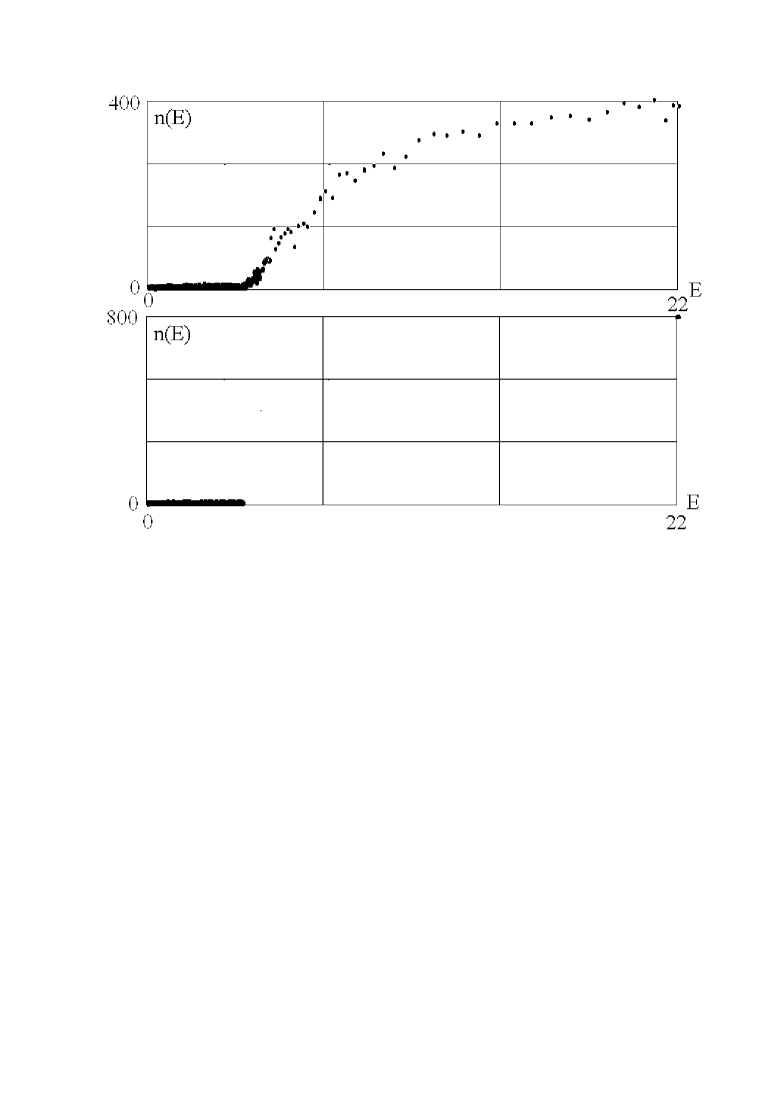
FIG. 1.: Energy dependance of number of sites covered by the wave function for the Hamiltonian (1) with $N=1000$, $\Delta=4$, $w(r)=v_{0}\exp-|r/R|$, $v_{0}=0.5$ , $R=20$ (top). The same for the Hamiltonian (5) with $v=2Rv_{0}=20$ (bottom).

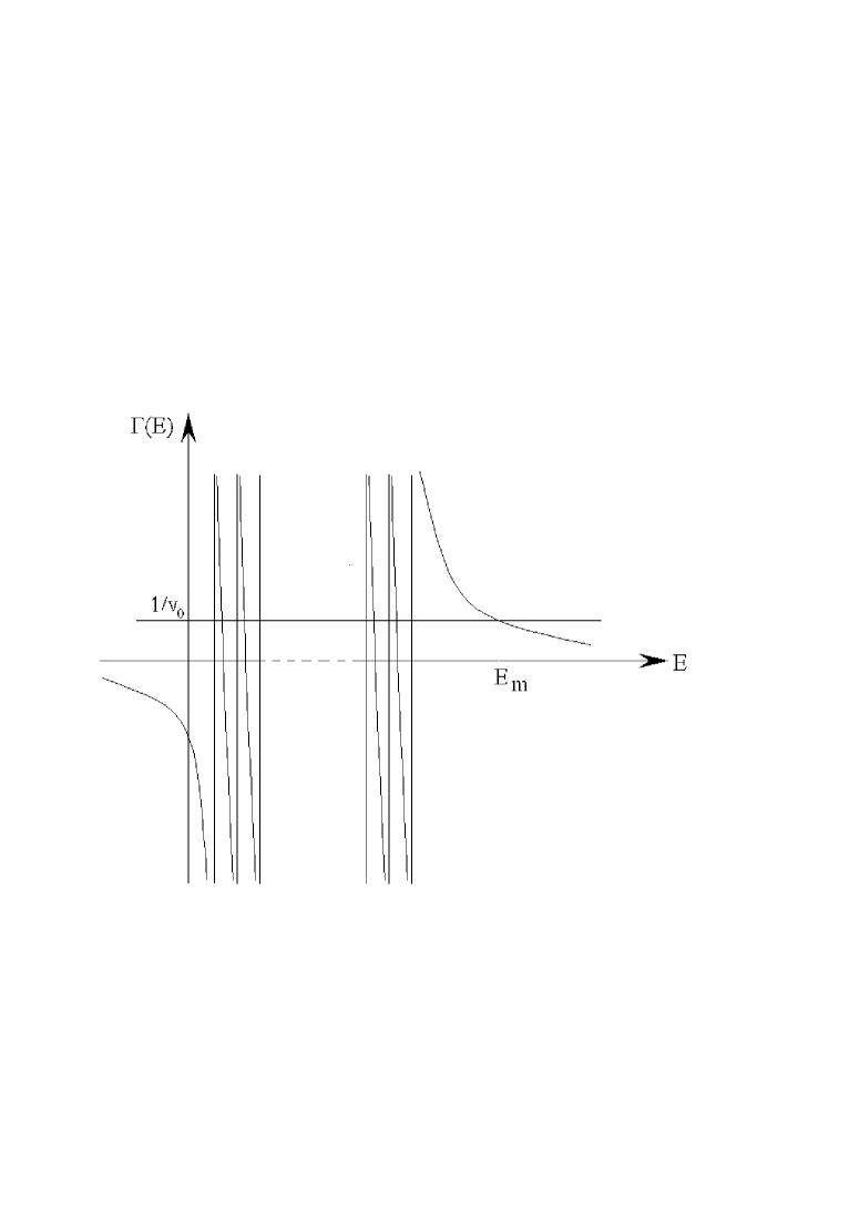
FIG. 2.:

REFERENCES

- [1] P.W.Anderson, Phys.Rev. 109, 1492 (1958)
- [2] arXiv: cond-mat/0303092 v2 9 Aug 2003
- [3] Phys.Rev.Lett., A.Rodriguez, V.A.Malyshev, G.Sierra, M.A. Anderson Transition in Low-Dimensional Disordered Systems Driven by Long-Range Nonrandom Hopping, v90, n2 2003.
- [4] I.M.Lifshits, S.A.Gredeskul, and L.A.Pastur, Introduction in Theory of Disordered Sysytems, Nauka, Moskow (1982)
- [5] Ved’aev A.V., Journal of Theoretical and Mathematical Physics, 1977, v. 31, p. 392
- [6] J.Phys. C: Solid State Phys. 1969. V. 2. P. 1717.
- [7] arXiv: cond-mat/9909335