Numerical Jordan-Wigner approach for two dimensional spin systems

Abstract

We present a numerical self consistent variational approach based on the Jordan-Wigner transformation for two dimensional spin systems. We apply it to the study of the well known quantum ($S=1/2$) antiferromagnetic $XXZ$ system as a function of the easy-axis anisotropy $\Delta$ on a periodic square lattice. For the $SU(2)$ case the method converges to a Néel ordered ground state irrespectively of the input density profile used and in accordance with other studies. This shows the potential utility of the proposed method to investigate more complicated situations like frustrated or disordered systems.

I Introduction

Quantum spin systems in two dimensional (2D) lattices have been the subject of intense research, mainly motivated by their possible relevance in the study of high temperature superconductors Anderson . On the other hand, high magnetic field experiments on materials with a 2D structure which can be described by the Heisenberg antiferromagnetic model in frustrated lattices have revealed novel phases as plateaux and jumps in the magnetization curves SrCuBo . In spite of the huge efforts made, a general understanding of the phase diagram of such magnets is elusive and it is then worth trying to develop new techniques to study these systems systematically. Among the many different techniques that have been used to study such systems, the generalization of the celebrated Jordan-Wigner (JW) transformation JW to two spatial dimensions Fradkin has some appealing features. It allows one to write the spin Hamiltonian completely in terms of spinless fermions in such a way that the $S=1/2$ single particle constraint is automatically satisfied due to the Pauli principle, while the magnetic field enters as the chemical potential for the JW fermions. The price one has to pay is the appearance of complicated non-local interactions between fermions. This method has been applied in ARF (see also Wang ) to study the $XXZ$ Heisenberg antiferromagnet. These studies have been reviewed in Derzhko .

More recently this technique was used to obtain a theoretical magnetization curve for the Shashtry-Sutherland model, reproducing at the mean field level some of the experimentally observed features for the material SrCu₂(BO₃)₂ which is assumed to be described by such model Misguich . Also the $J_{1}-J_{2}$ model, in relation to Li₂VOSiO₄ and Li₂VOGeO₄ compounds Chang , and the $XY$ model Derzhko2003 were analyzed with the same technique. All the studies performed have been based on a mean field decoupling scheme as the starting point to deal with the non-local interactions introduced by the JW transformation. In ARF the mean field procedure was further supplemented by the inclusion of fluctuations in terms of an auxiliary gauge field with a leading Chern-Simons dynamics coupled to the lattice fermions. However, in spite of the partial success of the JW transformation, many problems remain open, in particular in connection to the study of frustrated systems such as the triangular lattice, etc. In some cases, the results obtained via a direct mean field treatment lead to results that are believed to be incorrect, like the appearance of a spin gap in the triangular lattice case (see the discussion in Misguich ). The main problem associated with the JW approach is related to the implementation of the above mentioned mean field decoupling, which renders the description approximate. Another highly non-trivial problem is the construction of the lattice description of the Chern-Simons theory, which has been carefully studied for the square lattice case onlySemenoff .

It is the purpose of the present paper to propose a systematic self consistent mean field method for exploring the ground state (GS) of 2D lattice spin 1/2 systems, in a way that could be applied to arbitrary lattice topologies. The method can also be used in the presence of an external magnetic field, at finite temperature and even be applied to disordered systems.

II Jordan-Wigner transformation in $2$-dimensions

The Jordan-Wigner transformation in $2$ spatial dimensions was originally proposed in Fradkin as a generalization of the well known transformation in 1D, and has been further developed in ARF ; Wang . It maps a set of spin 1/2 operators $\vec{S}_{p}$ on lattice sites $p$ into spinless fermion operators $c_{p}$ by

$$S^{-}_{p} = c_{p}\exp\left[i\sum_{q\neq p}\theta_{qp}c^{\dagger}_{q}c_{q}\right]\ ,$$

$$S^{+}_{p} = c^{\dagger}_{p}\exp\left[-i\sum_{q\neq p}\theta_{qp}c^{\dagger}_{q}c_{q}\right]\ ,$$

$$S^{z}_{p} = c^{\dagger}_{p}c_{p}-1/2\ ,$$ (1)

where $S^{\pm}=S^{x}\pm iS^{y}$ are the usual spin raising and lowering operators and $\theta_{qp}$ is the argument of the vector drawn from site $p$ to site $q$. The transformation is non-local, and sets a preferred quantization axes $z$. The spin operators (1) satisfy bosonic $SU(2)$ commutation relations, while the Pauli principle ensures that they belong to the irreducible representation $S=1/2$. Indeed, the only necessary ingredient that ensures the $SU(2)$ commutation relations is the assignment of the phase factors which satisfies, for each pair of sites $p,q$

$$e^{i\theta_{pq}}\,e^{-i\theta_{qp}}=-1.$$ (2)

One should notice that there is a large freedom in choosing phase factors satisfying this condition (2). For instance, one could arbitrarily shift $\theta_{pq}\to\theta_{pq}+2k\pi$ with different integers $k$ for each pair of lattice points $p,q$, or even perform an arbitrary simultaneous rotation for $\theta_{pq}$ and $\theta_{qp}$. Standard plane angles $-\pi<\theta\leq\pi$ measured from the $x$ axis is just the simplest translation invariant choice on the flat infinite plane. It should be stressed that this large freedom does not alter the physical results, as long as all degrees of freedom are treated exactly. However, in any approximate treatment, this may introduce ambiguities that should be handled carefully, as we discuss below.

One salient feature of the JW transformation is that no constraint is needed on the new variables (cf. for instance the Holstein-Primakoff or Schwinger bosons), but non-locality is the main stumbling block in the approach.

The success of the JW transformation in $1$ spatial dimension, in spite of being non-local, resides on the fact that $XY$ nearest neighbors (NN) interactions become local in fermion variables; this is not the case in $2$ dimensions. Indeed, consider the $XY$ Hamiltonian on a given 2D lattice

$$H_{XY}=J\sum_{<p,q>}\left(S_{p}^{x}S_{q}^{x}+S_{p}^{y}S_{q}^{y}\right),$$ (3)

where $J$ is the exchange constant and the sum runs over all nearest neighbors $<p,q>$ on the lattice. In terms of fermion variables the Hamiltonian reads

$$H_{XY}=J\sum_{<p,q>}\left(\frac{1}{2}c^{\dagger}_{p}e^{i\hat{\alpha}(p,q)}c_{q}+H.c.\right),$$ (4)

where

$$\hat{\alpha}(p,q)=\sum^{\prime}_{r}(\theta_{rq}-\theta_{rp})c^{\dagger}_{r}c_{r}$$ (5)

(the ^′ on the sum indicates that $\theta_{rr}$ terms are absent). This phase is highly non local; in the 1D case, this same expression becomes local due to the fact that the only two actual values for the angles are $0$ and $\pi$. The non-locality in 2D is usually overtaken by the introduction of an auxiliary gauge field $A_{\mu}$, which on the one hand represents the phases in eq.(4) as the usual minimal coupling on the lattice, and on the other hand is governed by a Chern-Simons action. The Gauss law associated to the first order Chern-Simons action imposes a constraint which in anyon language attaches half a quantum flux to each fermion, providing the statistical transmutation of fermions into bosons. Then, a mean field treatment (known as average field approximation) of the gauge field can be done, leading in general to a quadratic NN interaction between fermionsARF . However, the Chern-Simons approach has serious difficulties when one deals with arbitrary lattice topologies (for example the triangular lattice), and the associated mathematical problems are not yet solved.

We do not introduce such an auxiliary gauge field, but keep working with fermion variables. In order to perform numeric computations, one has to set a finite size lattice and impose suitable boundary conditions. We use periodic boundary conditions, this leading to a lattice on the torus. Moreover, the lattice size should be compatible with possible periodic configurations; in the case of a square lattice, size must be even in order to not interfere with the possible Néel order.

Now, it is not straightforward to define the JW transformation on the torus Fradkin-Wen , as the vector joining two different points is not unique . As one has to take care of condition (2), the vectors joining $p$ with $r$ and $r$ with $p$ must have arguments differing in $\pi$. We have to choose a unique segment joining each pair of points $p,r$, and then draw both vectors along it. One can choose this segment by a criteria of minimal distance. However, there exist pairs of points on the torus that can be joined by two or more different segments with minimal distance and hence an ad-hoc criterion must be added. Any such criterion unavoidably breaks translation invariance, by preferring one segment over the rest. Naturally, we propose a criterion trying to minimize the violation of translation symmetry as follows: we set a principal finite size lattice and extend it on a plane by periodicity; for each point on the principal lattice we consider also its periodic copies. Now, given a pair of sites, we look for the shortest segment joining either the points or their copies; when such a segment is unique, the procedure is translationally invariant. For those pair of points where one can find more than one minimal distance segments, we choose the one with both ends belonging to the principal lattice, thus breaking translation invariance. Finally, the angles $\theta_{pr}$ and $\theta_{rp}$ are computed as the arguments of the vectors joining $p$ and $r$ along the chosen segment. For convenience we also define that $\theta_{pp}=0$, in order to handle the restriction on the sums in eqs.(1, 5).

As we mentioned in the Introduction, the JW transformation is exact but the resulting Hamiltonian is highly non-local and some kind of approximation is necessary to proceed.

We propose here a variational approach to deal with the non-local phases in eq.(4) and the quartic terms that can arise from $S^{z}$ interactions. Working directly with fermion variables, we replace the local fermionic occupation numbers $\hat{n}_{p}=c^{\dagger}_{p}c_{p}$ by their expectation values in an arbitrarily chosen variational state. This procedure leads to a multi-parameter mean field approach, that will in turn be evaluated self-consistently. This is the subject of the next section.

III Variational approach, applied to the $XXZ$ model

To describe in full detail the method laid down above, we apply it to a generalized quantum spin 1/2 Heisenberg antiferromagnet in a square 2D periodic lattice, defined by the Hamiltonian

$$\!\!\!\!H_{XXZ}=J\sum_{<p,q>}\left(S_{p}^{x}S_{q}^{x}+S_{p}^{y}S_{q}^{y}+\Delta S_{p}^{z}S_{q}^{z}\right)-h\sum_{p}S^{z}_{p},$$ (6)

where $\vec{S}_{p}=(S_{p}^{x},S_{p}^{y},S_{p}^{z})$ represents the $S=1/2$ spin operator at site $p$, $J>0$ is the exchange constant and $0<\Delta<\infty$ the “$XXZ$” anisotropy parameter. The first sum in (6) runs over all nearest neighbors in the given lattice, while the last term represents the interaction with a transverse external magnetic field $h$. We work on a periodic rectangular lattice of size $K=N_{x}\times N_{y}$.

Using the JW transformation defined in eq.(1), the Hamiltonian can be written in terms of spinless fermions as

$$H_{XXZ}=J\sum_{<p,q>}\left[\frac{1}{2}(c^{\dagger}_{p}e^{i\hat{\alpha}(p,q)}c_{q}+H.c.)+\Delta(c^{\dagger}_{p}c_{p}-\frac{1}{2})(c^{\dagger}_{q}c_{q}-\frac{1}{2})\right]-h\sum_{p}(c^{\dagger}_{p}c_{p}-\frac{1}{2})\ ,$$ (7)

where the phase $\hat{\alpha}(p,q)$ is defined in (5). Notice that the magnetic field $h$ plays the rôle of a chemical potential for the JW fermions. In particular, we look for the ground state of the system (7) with fixed global magnetization $M=0$ (corresponding to $h=0$).

We implement a self consistent mean field solution by starting with a given fermion distribution profile $\{n_{p}\}$t (which can be random or guided by some ansatz) on the lattice,

$$\langle\hat{n}_{p}\rangle=n_{p},$$ (8)

which has to satisfy a global constraint to provide the given magnetization (here $\sum n_{p}=K/2$ corresponds to $M=0$). We then replace the operator $\hat{\alpha}(p)$ by its expectation value

$$\langle\hat{\alpha}(p,q)\rangle=\sum_{r}(\theta_{rq}-\theta_{rp})\ n_{r},$$ (9)

where the angles $\theta_{pq}$ are assigned following the criterion presented in the previous section. To be precise, the principal lattice can be defined by indexing each site by a position pair $(i,j)$, and setting the range $i=0\cdots N_{x}-1$, $j=0\cdots N_{y}-1$. Periodic boundary conditions are then expressed by $(i,j)\equiv(i+N_{x},j)\equiv(i,j+N_{y})$.

Regarding the Ising term

$$S_{p}^{z}S_{q}^{z}=c^{\dagger}_{p}c_{p}c^{\dagger}_{q}c_{q}-\frac{1}{2}c^{\dagger}_{p}c_{p}-\frac{1}{2}c^{\dagger}_{q}c_{q}-\frac{1}{4}$$ (10)

in eq.(7), it is quartic in fermion operators, so we also treat it in mean field. In order to approximate the first term in (10) with a quadratic expression we propose the following

$$c^{\dagger}_{p}c_{p}c^{\dagger}_{q}c_{q}\to\frac{1}{2}(c^{\dagger}_{p}c_{p}\langle c^{\dagger}_{q}c_{q}\rangle+c^{\dagger}_{q}c_{q}\langle c^{\dagger}_{p}c_{p}\rangle),$$ (11)

supported by best results in a posteriori evaluation of the GS energy (some other possibilities are discussed in Derzhko ).

At this step, the Hamiltonian can be written as

$$H_{XXZ}^{(MF)}(\{n_{p}\})=\sum_{p,q}c^{\dagger}_{p}J_{pq}(\{n_{p}\})c_{q}+C$$ (12)

where

$$J_{pq}=\left\{\begin{array}[]{lr}\frac{J}{2}\,e^{i\alpha(p,q)}&{\rm if}<p,q>{\rm nearest\,neighbors}\\[5.69054pt] \frac{J\Delta}{2}(\sum_{neighbors\ \ q}\langle n_{q}\rangle-4)&{\rm if\,}p=q\\[5.69054pt] 0&{\rm otherwise}\end{array}\right.$$ (13)

and $C=KJ\Delta/2$.

The main idea of the present paper is to provide a systematic way to compute an approximation to the true GS. We first find the GS for the quadratic $H_{XXZ}^{(MF)}(\{n_{p}\})$ by solving the one particle (1P) spectrum and filling the system with the lowest energy 1P states, up to the proper filling fixed by the total magnetization $M$. Then we compute from this approximate GS a new set of local densities $n^{\prime}_{p}=\langle GS|c^{\dagger}_{p}c_{p}|GS\rangle$, which we use as a new input in (12) and iterate this procedure looking for a fixed point configuration for the density profile, i.e. a set of local densities $\{n^{*}_{p}\}$ satisfying

$$n^{\prime}_{p}(\{n^{*}_{q}\})=n^{*}_{p}\ .$$ (14)

The existence of a fixed point solution for this mapping and its eventual dependence on a given initial configuration is not at all obvious and has to be studied numerically.

In order to proceed with the method, $H_{XXZ}^{(MF)}(\{n_{p}\})$ can be written in diagonal form

$$H_{XXZ}^{(MF)}(\{n_{p}\})=\sum_{k=1}^{K}\epsilon(k)\ d^{\dagger}_{k}d_{k}+{\rm constant}$$ (15)

where $\epsilon_{k}$ are the 1P eigenvalues of the quadratic part of $H_{XXZ}^{(MF)}$. Notice that $k$ is just an integer index over the spectrum, not to be confused with the lattice momentum. Moreover, we order the eigenvalues ascendently.

The operators $d_{k}$ are related to $c_{p}$ by

$$d_{k}=\sum_{p}Q^{*}_{kp}c_{p}$$ (16)

where $Q_{pk}$ is the matrix of eigenvectors of $J_{pq}$. We compute both $\epsilon_{k}$ and $Q_{pk}$ numerically. Being $Q$ unitary, the set of $d_{k}$ operators satisfy fermion commutation relations, $\{d_{k},d^{\dagger}_{k^{\prime}}\}=\delta_{kk^{\prime}}$. Moreover, the total fermion number operator satisfies

$$N=\sum_{p=1}^{K}c^{\dagger}_{p}c_{p}=\sum_{k=1}^{K}d^{\dagger}_{k}d_{k},$$ (17)

making it easy to control the filling in terms of the new fermions.

We now construct the approximation to the quantum GS as the half-filled state that minimizes the energy, namely

$$|GS\rangle=\prod_{k=1}^{K/2}d^{\dagger}_{k}|0\rangle$$ (18)

Notice that this is a well defined quantum state of $K/2$ particles, except for casual degeneracy of the 1P spectrum at the Fermi level . This is not the case for the $XXZ$ model on the square lattice (see details below).

From $|GS\rangle$ it is now easy to compute the approximate GS energy, as

$$E_{GS}=\langle GS|H_{XXZ}^{(MF)}|GS\rangle=\sum_{k<K/2}\epsilon_{k}+C.$$ (19)

Also the local occupation numbers can be computed in this approximate GS as

$$n^{\prime}_{p}=\langle GS|c^{\dagger}_{p}c_{p}|GS\rangle=\sum_{k<K/2}Q^{*}_{pk}Q_{pk}.$$ (20)

With these occupation numbers we start again the procedure: compute $J_{pq}$ in MF, diagonalize the new $H_{XXZ}^{(MF)}$, etc.

We have found after thorough numerical investigations that a fixed point solution for eq.(14) always exists, but metastable solutions can also appear, depending on the initial configuration one chooses. In any case, one can distinguish metastable solutions from the best GS approximation simply by comparing their energies. Moreover, we describe below how this drawback can be naturally solved by introducing a thermal bath to kick the system out from the vicinity of metastable states.

Indeed, one can consider the effects of finite temperature by replacing the proposed ground state (18) by a thermal state $|\Psi_{\beta}\rangle$, compatible with the Fermi-Dirac 1P energy distribution at a given temperature,

$$n(\epsilon)=\frac{1}{1+\exp(\beta(\epsilon-\bar{\epsilon}))},$$ (21)

where $\bar{\epsilon}$ is the 1P Fermi energy at half filling, and $\beta=1/kT$ is the inverse temperature. In detail, this thermal state $|\Psi_{\beta}\rangle$ is constructed as

$$|\Psi_{\beta}\rangle=\prod_{k\in\sigma}d^{\dagger}_{k}|0\rangle,$$ (22)

where $\sigma$ is a set of $K/2$ 1P states chosen with probability $n(\epsilon(k))$ from some random simulation.

An exploration of the Hilbert space of the system by constructing a thermal state from a starting fermion distribution, computing from it the new local fermion distribution and again constructing a thermal state should be considered as a thermalization at the given temperature. It provides a source of thermal noise that has proven to help the system in finding lower energy fixed points.

The thermalization can be done through several steps at a given temperature, and then quenching to the pure quantum regime ($T=0$), or it can be implemented by gradually lowering $T$ (annealing).

Besides, results at finite $T$ can also be achieved, by constructing an statistical ensemble of microscopic states compatible with $T$. Observables should then be computed as averages over the statistical ensemble. We do not attempt to complete this program in the present paper.

IV Results

We have tested the iterative approach described in the previous section with the well known anisotropic $XXZ$ model on periodic 2D square lattices of size up to $20\times 20$ sites, at zero total magnetization. The sizes of the lattice that we explored are by no means an upper limit, as our computations were made on a modest computer. The anisotropy parameter $\Delta$ has been explored in a range from $0.05$ to $1.5$, including the isotropic $SU(2)$ case ($\Delta=1$, Heisenberg model). As starting configurations $\{n_{p}\}$ we have used random, uniform, and different amplitude staggered distributions. We performed several iterations and analyzed the evolution of the local fermion profile and the approximate GS energy. We report the results in terms of spin variables, noting that the local fermion occupation represents the local magnetization as $m_{z}(p)=(n_{p}-\frac{1}{2})$.

Working at $T=0$, we have found that in general, from different starting configurations, the system rapidly finds a Néel order as stable ground state approximation, after $15\sim 20$ iterations. The Néel order parameter, usually defined as the staggered or sublattice magnetization $m_{z}$, depends on the anisotropy parameter $\Delta$. Fluctuations around this staggered magnetization are typically of order $10^{-8}$. In figure (1) we plot the Néel order parameter $m_{z}$ of the fixed point solution for different values of $\Delta$, for several lattice sizes.

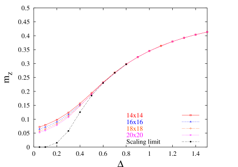
Figure 1: Néel order parameter at fixed points, in function of the anisotropy $\Delta$. Several lattice sizes and the scaling limit are shown.

Finite size effects are noticeable for lower values of $\Delta$, so we also show the results of a finite size scaling $m_{z}(\infty)$ of our data, fitted with a power law $m_{z}(K)=m_{z}(\infty)+c/K^{\alpha}$. The corresponding GS energies per site are shown in figure (2) where one observes that scaling with the system size is clearly less important.

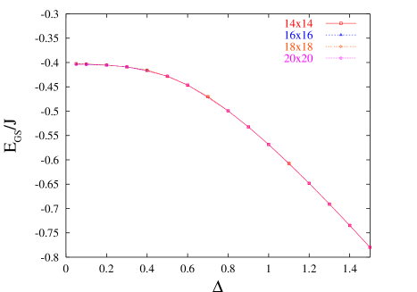
Figure 2: GS energy, in function of the anisotropy $\Delta$. Data corresponds to configurations plotted in figure (1).

We have observed that the 1P spectrum of the mean field Hamiltonian (12) presents a gap $2m_{z}J\Delta$ for Néel ordered configurations, at the half filling Fermi level. This is in agreement with (ARF ) and makes the construction of $|GS\rangle$ in eq.(18) unambiguous.

In the case of random initial distributions, metastable configurations can show up; a detailed inspection of the local magnetization in these cases reveals the formation of antiferromagnetic domains, that is the presence of the two possible Néel configurations in different regions. In figure (3) we show an example of such domains, at two different stages of a sample evolution. It is natural to expect that larger lattices favor the formation of these domains, as it indeed is observed. These configurations have higher energy than the uniform Néel state and correspond then to metastable configurations; correspondingly, they are not presented in figures (1, 2).

Figure 3: Occupation patterns for a metastable configuration, where antiferromagnetic domains appear. The size of the points is proportional to the local fermion occupation number. This configurations occurred on a $20\times 20$ lattice, with $\Delta=1.1$, after 10 steps of thermalization at $T=0.2~{}J$, and 10 (left panel) or 20 (right panel) more steps of GS search at $T=0$. The smaller domain is seen to decrease in size under the simulated evolution.

When a thermal bath is simulated on random initial configurations, we have observed that metastable configurations are less likely to appear. After thermalization we let the system to cool down by either quenching or annealing as described in Section III, and complete the iterations at $T=0$. In fact, a few steps ($\sim 10$) of thermalization with sufficiently high $T$ completely avoid domain formation and lead to a unique fixed point mean field configuration; the required temperature is higher for larger lattices, being of the order of $J$ for the lattice of $20\times 20$. We have checked that under general circumstances, quenching provides the fastest convergence method to the minimum energy state. An example of the evolution of the Néel order parameter from an initial random configuration, under thermalization with different temperatures, is shown in figure (4).

Figure 4: Example of the evolution of the Néel order parameter from a sample initial random configuration. Data corresponds to the system depicted in fig.(3), with a vertical line separating the thermal evolution and the $T=0$ evolution. Error bars indicate the standard deviation of local magnetization from Néel order (reduced by a factor of 5 for clarity). Insufficient thermalization can lead to metastable configurations or to very slow convergence, while higher temperature dramatically improves convergence towards an ordered configuration.

The results of the present MF computation show all the features expected for the Heisenberg antiferromagnet on the square lattice. They are of course not comparable to accurate numerical techniques Cuccoli , but are in qualitative agreement with results from previous studies. In particular, in the scaling limit we obtain no Néel order for small anisotropy $\Delta$, where the system presumably has $XY$ order. We can estimate a critical value $\Delta^{*}\approx 0.2$, above which Néel order develops. For the isotropic Heisenberg point $\Delta=1$ we obtain a sublattice magnetization $m_{z}=0.3453$, with ground state energy per site $E_{GS}/K=-0.5683J$, to be compared for instance with corresponding Quantum Monte Carlo values of $0.307$ and $-0.6694J$ QMC .

V Conclusions

We have presented a self consistent MF procedure for exploring the quantum ground state of any $S=1/2$ spin system on a 2D lattice. When tested on the $XXZ$ model on a square lattice, the method provides the correct qualitative description of the system, with no a priori ansatz for any kind of order. We computed the values for the sublattice magnetization and GS energy for a wide range of values of the anisotropy parameter, which compare qualitatively well with the available numerical data, at least for $\Delta=1$ where most accurate data is available. Moreover, we have found that the sublattice magnetization as a function of the $XXZ$ anisotropy shows the correct qualitative behaviour, expected from a spin wave analysis ARF .

The present approach has a more general scope than previous MF computations, in the sense that it can be applied to any lattice topology, irrespectively of the appearance of frustrating units, a fact that prevents the applicability of one of the most powerful numerical techniques such as Quantum Monte Carlo. A magnetic field can be trivially added as a chemical potential for the JW fermions and hence magnetization curves could be obtained. Since the method is not based on any periodicity of couplings, it can be well suited to study disordered quantum spin systems, at the only price of increasing the CPU time. Last but not least, the approach is naturally well suited for the study of the thermodynamics of these systems, since temperature can be added in a simple way.

Among other situations, it would be interesting to apply this technique to the Heisenberg quantum AF on the triangular lattice, where there is disagreement between Chern-Simons MF predictions Misguich and numerical data about a magnetization plateaux at zero magnetization. Another case of interest the kagomé lattice, where a quantum spin liquid is believed to be realized Lluillier (see also ojo ). This issues will be investigated elsewhere.

Acknowledgements: We are especially grateful to M. Grynberg and A. Honecker for useful discussions and computational help. We also thank C. Balseiro, W. Brenig, J. Drut and E. Fradkin for useful comments. We acknowledge CONICET and Fundación Antorchas (grants No. 14116-11 and 14022-79) for financial support, and the Ecole Normale Supérieure de Lyon, where part of this work was done.

References

- (1) P.W. Anderson, Science 235, 1196 (1987).
- (2) K. Onizuka et al., J. Phys. Soc. Jpn. 69, 1016 (2000).
- (3) P. Jordan, E.P. Wigner, Z. Phys. 47, 631 (1928).
- (4) E. Fradkin, Phys. Rev. Lett. 63, 322 (1989).
- (5) A. Lopez, A.G. Rojo, E. Fradkin, Phys. Rev. B 49, 15139 (1994).
- (6) Y.R. Wang, Phys. Rev. B 43, 3786 (1991); 45, 12604 (1992); 45, 12608 (1992); K. Yang, L.K. Warman, S.M. Girvin, Phys. Rev. Lett. 70, 2641 (1993).
- (7) O. Derzhko, J. Phys. Studies (L’viv) 5, 49 (2001).
- (8) G. Misguich, Th. Jollicoeur, S.M. Girvin, Phys. Rev. Lett. 87, 097203 (2001).
- (9) M-C. Chang, M-F. Yang, Phys. Rev. B66, 184416 (2002).
- (10) O. Derzhko, T. Verkholyak, R. Schmidt, J. Richter, Physica A320, 407 (2003).
- (11) J. Ambjorn, G. Semenoff, Phys. Lett. B226, 107 (1989).
- (12) Related problems in the gauge field approach were discussed in X.G. Wen, E. Dagotto, E. Fradkin, Phys. Rev. B 42, 6110 (1990).
- (13) A. Cuccoli, T. Roscilde, V. Tognetti, R. Vaia, P. Verruchi, J. Appl. Phys. bf 93, 7640 (2003).
- (14) M. Calandra Buonaura, S. Sorella, Phys. Rev. B 57, 11446 (1998).
- (15) Ch. Waldtmann, H.-U. Everts, B. Bernu, P. Sindzingre, C. Lhuillier, P. Lecheminant, L. Pierre, Eur. Phys. J. B 2, 501 (1998)
- (16) P. Nikolic, T. Senthil, preprint cond-mat/0305189.