Testing the Stability of the 2000 US Stock Market “Antibubble”

Abstract

Since August 2000, the stock market in the USA as well as most other western markets have depreciated almost in synchrony according to complex patterns of drops and local rebounds. In [1], we have proposed to describe this phenomenon using the concept of a log-periodic power law (LPPL) antibubble, characterizing behavioral herding between investors leading to a competition between positive and negative feedbacks in the pricing process. A monthly prediction for the future evolution of the US S&P 500 index has been issued, monitored and updated in [2], which is still running. Here, we test the possible existence of a regime switching in the US S&P 500 antibubble. First, we find some evidence that the antibubble has exhibited a transition in log-periodicity described by a so-called second-order log-periodicity. Second, we develop a battery of tests to detect a possible end of the antibubble of the first order which suggest that the antibubble was alive in August 2003 but has ended in the USA, when expressed in the local US dollar currency. Our tests provide quantitative measures to diagnose the end of an antibubble. Such diagnostic is not instantaneous and requires from three to six months within the new regime before assessing its existence with confidence. From the perspective of foreign investors in their currencies (S&P500 denominated in British pound or in euro) or when expressed in gold so as to correct for an arguably artificial US$ valuation associated with the Federal Reserve interest rate and monetary policy, we find that the S&P 500 antibubble is still alive and running its course. Similar analyses performed on the major European stock markets (CAC 40 of France, DAX of Germany, and FTSE 100 of United Kingdom) show that the antibubble is also present and continuing there.

,

1 Introduction

In 1999, in order to describe the evolution of the Japanese stock market since its all-time high in December 1989, Johansen and Sornette introduced the concept of an “antibubble” as a counterpart of a bubble resulting from the same herding behavior and characterized by log-periodic power-law (LPPL) structures but with decelerating (rather than accelerating) oscillations [3]. The term “antibubble” is inspired by the concept of “antiparticle” in physics. Just as an antiparticle is identical to its sister particle except that it carries exactly opposite charges and destroys its sister particle upon encounters, an antibubble is both the same and the opposite of a bubble; it’s the same because similar herding patterns occur, but with a mostly bearish versus bullish slant. Some antibubbles can also describe increasing markets over long times, although a bearish phase is more commonly recognized in the markets [4, 5, 6, 7]. In August 2002, we detected the existence of a clear signature of an antibubble in the relaxation of the US S&P 500 index since August 2000 with high statistical significance, in the form of strong log-periodic components [1]. Similarly to the prediction offered in [3] for the evolution of the Nikkei index which was later evaluated in [8], we presented a prediction for the future evolution of the US S&P 500 index [1, 6]. This prediction has been monitored and updated once a month at the URL [2]. Accompanying the US stock markets, the antibubble regime since 2000 seems to be a world-wide phenomenon in the major western stock market [4]. These works on antibubbles extend a large amount of theoretical and empirical work on LPPL bubbles which often end in crashes or strong corrections (see [9, 10, 11, 12] and references therein). In this context, Roehner has investigated the resilience pattern around large price peaks [13] and has found strong negative correlations between stock market crash-recovery and interest rate spread [14].

In contrast to a LPPL bubble whose end is automatically described by one of the parameters, the critical time $t_{c}$, the LPPL formulation of an antibubble does not say anything a priori about its duration. For prediction purpose, the agonizing question is whether the detection of an antibubble pattern ensures its continuation in the future and for how long. In the case of the Japanese antibubble studied in depth [3, 8], the detection was performed in early January 1999, corresponding to 9 years since the birth of the antibubble. The prediction issued in early January 1999 turned out to be followed subsequently ex-ante by the Nikkei index over more than two years. However, in January 1999, it was hard a priori to assess for how long the theory would be a correct predictor of the future evolution of the Nikkei index.

Here, we address this question of the detection of a change of regime from an antibubble phase to something else. For this purpose, the present situation is perhaps more favorable than for the Nikkei in January 1999 for the following reason. As we said above, in January 1999, the antibubble has been unfolding itself already for 9 years. It was found necessary to extend the LPPL theory from a first-order log-periodic formula to a second-order and then to a third-order formula. It should be stressed that the first-order formula is embedded as a special case of the second-order formula which is itself embedded as a special case of the third-order formula. The logic of this succession of formulas is that they represent successive improvement to describe the market price at time intervals further and further away from the early development of the antibubble. The larger is the order of the formula, the larger is the time interval over which the theory applies. The prediction issued in January 1999 was performed based on the third-order LPPL formula. In contrast, the analysis of the US S&P 500 antibubble has been performed much earlier after about only $2.5$ years since its inception in August 2000 [1]. Due to this relatively short time span, it was found that the first-order formula was sufficient to describe the empirical data, while the second-order (and a fortiori the third-order) formula was not needed as it did not lead to any statistically significant improvement. We thus concluded that the S&P 500 index had not yet entered into the second phase in which the angular log-frequency may start its shift to another value, as did the 1990 Nikkei antibubble after about 2.5 years. However, this situation offers the possibility for tracking a possible future change of regime from the first-order to the second-order formula. This is the first purpose of this paper. Using data garnered over ten additional months, we show that one can start to detect the occurrence of such a change of regime. Adding an additional year of data confirms further this conclusion, as we shall show. The statistical tests described below give the probability to reject the hypothesis that the market has not entered the second phase in which the angular log-frequency is shifting to another value. These results suggest the possibility that, indeed, we have entered a cross-over regime in log-frequency shift. The improved second-order log-periodic formula has implications in the prediction of the future drops of the markets.

The second purpose of our paper is to develop a battery of tests to gain a better understanding of which scenario might be the most likely to unfold: is the antibubble likely to continue and is the market when expressed in one of the major foreign currencies or in gold to drop further? Or will the stock market transit to another regime, perhaps rebound to develop a new bullish regime? Or even worse (from the point of view of our model): is it possible that the US and European stock market has already entered a regime different from that described by the LPPL antibubble and that we have not yet taken this into account in our updates presented in [2]? The present paper provides the theoretical basis and the statistical anchor underlying the monthly prediction updates which are available at the URL [2].

2 Angular log-periodic frequency shifting?

2.1 First- and second-order LPPL formulas

Let us begin by recalling the mathematical expression of the price evolution trajectory of an antibubble [3, 1]:

$$\ln[p(t)]=A+B\tau^{m}+C\tau^{m}\cos\left[\omega\ln(\tau)+\phi\right]+\epsilon(t)~{},$$ (1)

where $p(t)$ is the price, $\epsilon(t)$ is the noise or fit residuals, $\omega$ is the angular log-frequency, $B<0$ for (bearish) antibubbles of interest here, $m$ is positive to ensure a finite price at the critical initiation time $t_{c}$ of the antibubble, $\phi$ is a phase which can be absorbed in a re-definition of the unit of the time, and $\tau=t-t_{c}$ is the distance to the critical time $t_{c}$ or onset of the antibubble.

As explained for instance in [9, 10, 11, 12], the power law acceleration $B\tau^{m}$ and log-periodicity $\cos\left[\omega\ln(\tau)-\phi\right]$ are both intimately linked to behavioral herding of agents whose investments involve a competition between positive and negative feedbacks [15, 16] leading to a critical point. Close to criticality, the “order parameter” $F\equiv\ln[p(t)]$ can be expanded according to a so-called Landau expansion [17] as a function of the “control parameter” $\tau$

$$\frac{dF(\tau)}{d\ln\tau}=\alpha F(\tau)+\beta|F(\tau)|^{2}F(\tau)...~{},$$ (2)

where the coefficients $\alpha$ and $\beta$ can, on general ground, be complex. Starting with the Landau expansion close to the critical point $\tau=0$, keeping only the first-order term $\alpha F(\tau)$ retrieves Eq. (1). Inclusion of the second-order term $\beta|F(\tau)|^{2}F(\tau)$ leads to [17]

$$\ln[p(t)]\approx A+\frac{B\tau^{m}+C\tau^{m}\cos\left\{\omega\ln\tau+\frac{\Delta_{\omega}}{2m}\ln\left[1+\left(\frac{\tau}{\Delta_{t}}\right)^{2m}\right]+\phi\right\}}{\sqrt{1+\left(\frac{\tau}{\Delta_{t}}\right)^{2m}}}~{},$$ (3)

where $\Delta_{\omega}\to 0$ and $\Delta_{t}\to\infty$ for $|\beta|\to 0$. Higher-order terms in the Landau expansion (2) can be taken into account to describe the behavior at long times further away from the critical point $t_{c}$, as done for the Nikkei antibubble [3].

2.2 Statistical tests

The question, whether the S&P 500 index has entered or not the second phase in which the angular log-frequency is shifting to another value, amounts to comparing the quality of the fits of the data with the first-order (1) and with the second-order formula (3).

Since the hypothesis that the S&P 500 index follows the first-order formula (1) is imbedded within the hypothesis that it follows the second-order formula (3), we can use the general theory of nested hypothesis testing. Calling $\chi_{1}$ and $\chi_{2}$ the root-mean-squares of OLS (ordinary least-squares) fits with (1) and (3) of the price time series of the S&P 500 index with length $n$, the likelihood-ratio or Wilks test states that the log-likelihood-ratio $T(\kappa)=2n\ln(\chi_{1}/\chi_{2})$ follows the chi-square distribution with $\kappa=2$ degrees of freedom, asymptotically when $n$ tends to infinity.

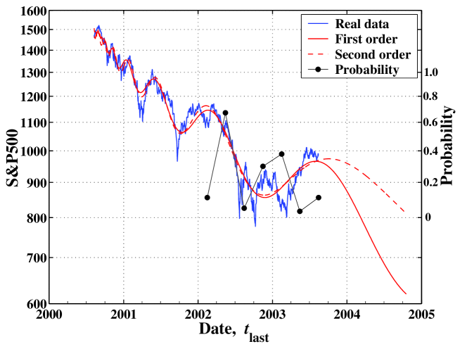
Figure 1: Left ordinate: Fits of the S&P 500 index over a time interval of three years with a daily sampling rate using the first-order LPPL formulae (1) and the second-order LPPL formulae (3). The parameters are the following: $t_{c}={\rm{2000/08/27}}$, $m=0.72$, $\omega=9.2$, $\phi=4.62$, $A=7.3123$, $B=-0.0037$, $C=-0.0008$, and the r.m.s. of fit residuals is $\chi_{1}=0.03859$ for the first order formula; and $t_{c}={\rm{2000/08/06}}$, $m=0.76$, $\omega=11.4$, $\phi=1.03$, $\Delta_{t}=2778$, $\Delta_{\omega}=-22.6$, $A=7.3245$, $B=-0.0031$, $C=-0.0007$, and the r.m.s. of fit residuals is $\chi_{2}=0.03729$ for the second order formula. Right ordinate: The probability that the simulated log-likelihood-ratio exceeds the realized ratio as a function of $t_{\rm{last}}$.

We first present the fits of the S&P 500 index time series from 2000/08/09 to 2003/08/15 with the first-order (1) and with the second-order formula (3) in Fig. 1. We will extend below the upper time limit of the fitting interval to provide further tests. The corresponding values $\chi_{1}=0.03859$ and $\chi_{2}=0.03729$ give a log-likelihood ratio $T=51$. The probability that $T$ is greater than 51 for a chi-square distribution with two degrees of freedom is $\approx 8\times 10^{-12}$, giving an extremely high confidence level undistinguishable from $1$. It seems that the second-order formula (3) is absolutely necessary. However, the rather large value of the cross-over time $\Delta_{t}=2778$ days = 7.6 years compared with the three year span of the time series suggests that the transition from the first-order (1) and with the second-order formula (3) has just begun in 2003/08/15. Redoing the calculation of the log-likelihood ratio $T$ for a shorter period also gives an extremely large confidence level, which is suspect. For such a finite-time series, the validity of the asymptotic Wilks test is questionable, especially in view of the non-Gaussian and the large dependence in the residues of the fits, which can be seen with the naked eye in Fig. 1. Wilks test assumes i.i.d. random residues, which is certainly not the case at the daily scale. For a weekly time step, the residues are less correlated. Redoing the fits using a weekly time scale, we obtain $T=8.7$, giving a confidence level of $98.7\%$. This enormous change in the confidence level casts doubts on the validity of the Wilks test and does not allow us to conclude from it that the second-order formula is necessary. More generally, because the price time series have a very complicated nature, applying classical statistical tests (like the Wilks test) to such time series is very dangerous. It is thus desirable to develop simple and robust (multivariate) statistics (defined in a moving time window). This paper is a first step in this direction.

To assess the statistical significance of the second-order formula, we propose the following alternative algorithm which is tailored to address the impact of the noise structure up to monthly time scales.

1. Starting the fit with the first-order formula, we decompose the residues in segments of one-month duration.

2. We reshuffle the one-month intervals of the residuals at random. Since there are about three years of data = 36 months, there are $36!$ (factorial of $36$) ways of reshuffling the monthly residues.

3. We add the reshuffled residues to the first-order formula, which provides us with a noisy synthetic log-periodic time series.

4. We fit this synthetic time series with the first- and with the second-order formulas and calculate the corresponding log-likelihood ratio $T$ for these two fits for this realization.

5. We redo steps 2-4 one thousand times and count how many times the value empirical value $T=51$ is exceeded.

This algorithm is nothing but a bootstrap with noise realizations generated from the real data. In this way, we keep the genuine structure of the dependence of real prices up to the monthly scale. This allows us to test how the empirical dependence structure of prices up to one month scale may interfere with the detection of log-periodicity and of its frequency shift. The monthly scale is a compromise between having many statistical realizations (favoring smaller time intervals) and keeping as much as possible all the idiosyncratic textures of the price times series that decorate the large scale log-periodicity.

We perform 1000 simulations for the S&P 500 index time series from 2000/08/09 to $t_{\rm{last}}=\rm{2003/08/15}$. The averages and standard deviations of the parameters obtained from the fits with Eq. (1) are the following: $\langle{t_{c}}\rangle=\rm{2000/08/19}\pm 19~{}\rm{days}$, $\langle{m}\rangle=0.72\pm 0.10$, $\langle{\omega}\rangle=9.4\pm 0.5$, $\langle{\phi}\rangle=3.33\pm 1.69$, $\langle{A}\rangle=7.32\pm 0.03$, $\langle{B}\rangle=-0.048\pm 0.32$, $\langle{C}\rangle=0.0010\pm 0.0006$, $\langle{\chi_{1}}\rangle=0.0363\pm 0.0013$. The averages and standard deviations of the parameters obtained from the fits with Eq. (3) are the following: $\langle{t_{c}}\rangle=\rm{2000/08/14}\pm 19~{}{\rm{days}}$, $\langle{m}\rangle=0.76\pm 0.11$, $\langle{\omega}\rangle=9.7\pm 1.7$, $\langle{\phi}\rangle=3.24\pm 2.08$, $\langle{\Delta_{t}}\rangle=5889\pm 2674$ days, $\langle{\Delta_{\omega}}\rangle=-3.7\pm 40$, $\langle{A}\rangle=7.32\pm 0.03$, $\langle{B}\rangle=-0.0039\pm 0.0029$, $\langle{C}\rangle=0.0009\pm 0.0006$, $\langle{\chi_{2}}\rangle=0.0358\pm 0.0014$. The average and standard deviation of the log-likelihood ratio are $\langle T\rangle=22.7\pm 25.8$. The probability that $T>51$ is found to be $11.1\%$. Thus, according to this bootstrap method, the null hypothesis that S&P 500 has not experienced a log-periodic frequency shift cannot be rejected at a significance level of 10%. However, the null hypothesis can be rejected at a significance level of 12%. Thus, the situation is less clear than with the Wilks test which assumes asymptotic Gaussian i.i.d. noise statistics but the evidence suggests that the transition to a log-periodic frequency shift has started. This has an important implication for the future evolution of the S&P 500 index, as the first-order (continuous line) and second-order (dashed line) formulas diverge significantly after 2003/08/15, as shown in Fig. 1.

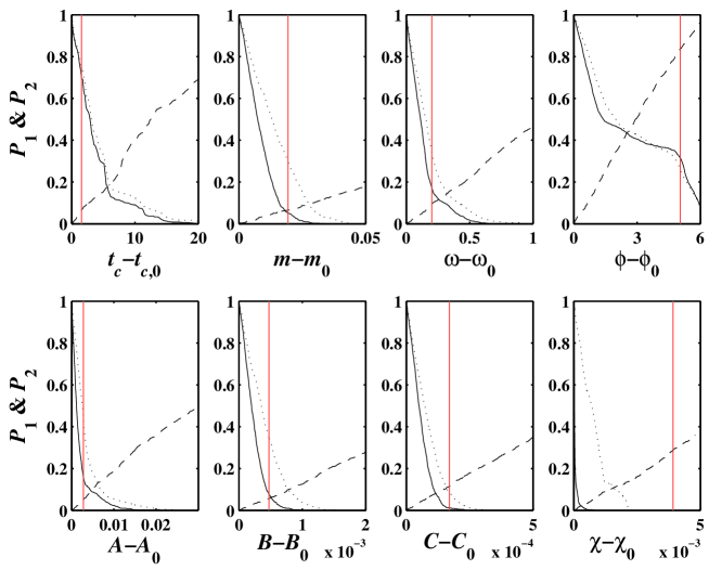
Figure 6: Same as Fig. 4 for $t_{\rm{last}}={\rm{2002/08/15}}$.

We have performed exactly the same procedure for other $t_{\rm last}$ chosen earlier than 2003/08/15, from $t_{\rm last}=$2002/02/15 to $t_{\rm{last}}=\rm{2003/08/15}$ in step of 3 months, giving a total of 7 time periods. For each $t_{\rm{last}}$, we calculate the empirical log-likelihood ratio and the associated probability ${\rm{Pr_{t_{\rm last}}}}$ that this ratio is exceeded, by using the above bootstrap method. This gives: ${\rm{Pr_{2002/02/15}}}=11\%$, ${\rm{Pr_{2002/05/15}}}=67\%$, ${\rm{Pr_{2002/08/15}}}=5.1\%$, ${\rm{Pr_{2002/11/15}}}=30\%$, ${\rm{Pr_{2003/02/15}}}=38\%$, ${\rm{Pr_{2003/05/15}}}=3.4\%$, and ${\rm{Pr_{2003/08/15}}}=11\%$. The plot of ${\rm{Pr}}_{t_{\rm{last}}}$ as a function of ${t_{\rm{last}}}$ is shown in Fig. 1, with the scale indicated on the right vertical ordinate. Overall, ${\rm{Pr_{t_{\rm last}}}}$ tends to decrease, which implies a progressive increasing relevance of the second-order formula compared with the first-order formula. The small value of ${\rm{Pr_{2002/02/15}}}$ is caused by the distortion of the prices with a local trough around 2002/02/15, while that of ${\rm{Pr_{2002/08/15}}}$ results from the local sharp peak around 2002/08/15 and probably the preceding crash as well. This effect has been observed in [18] (see Fig. 6 therein).

These results open seriously the possibility that the S&P 500 index has started to cross-over from the first-order to the second-order formula already in 2003/08/15. The corresponding fits shown in Fig. 1 suggests that there could be a delay in the drop predicted in 2003/08/15 on the sole basis of the first-order formula and perhaps a change of regime. In hindsight, we know now that the change of regime turned out to be of a different more subtle nature, as we discuss below.

As a word of caution, it is necessary to stress that the bootstrap method is an in-sample method. In-sample results can differ significantly from out-of-sample results because the bootstrap method is performed under a fixed sample. In particular, it gives conditional probabilities that converge to unconditional probabilities only as the sample size tends to infinity. It is difficult to assess a priori how close are bootstrap probabilities to unconditional probabilities in our finite sample. This remains a limitation of the approach.

3 How to detect the end of the antibubble?

3.1 Evolution of the fit parameters

According to standard economic theory, the prices of stocks must reflect the discounted future capital flows. In practice, the prices include the impact of news, from which anticipation on future cash flows is made, as well as behavioral biases and herding among investors. This provides a mixture of endogeneity and exogeneity [19, 11]. The antibubble phase is supposed to reflect mostly the impact of the behavioral part which leads to self-reinforced pessimism intermittently interrupted by transient phases of optimism.

If the antibubble pattern is to be a correct description of the market prices, a necessary condition is that its parameters should be robust, that is, approximately constant as a function of time. On the other hand, as time flows, the cumulative effect of exogenous news may detune progressively the antibubble pattern. This phenomenon may be accelerated in the presence of a strong exogenous shock. One can thus view the unfolding of an antibubble as a dynamic process with competing forces attempting to maintain and to destroy the LPPL structure.

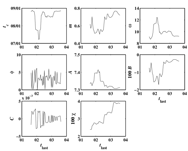
Figure 2: Evolution of the parameters of the fit of the S&P 500 with the log-periodic formula (1) as a function of time. Note that the tick labels on the ordinate of the left-top plot is “mm/dd” for year 2000 whereas the labels on the ticks of the abscissa refer to the last two digits of the years. Each tick is positioned of 1st January.

We fit the US S&P 500 index to the LPPL formulae (1) over a running window from 2000/08/09 to $t_{\rm{last}}$, where $t_{\rm{last}}$ is sampled at a bi-weekly rate in the interval from 2001/08/15 to 2003/08/15. Figure 2 shows the evolution of the fit parameters $t_{c}$, $m$, $\omega$, $\phi$, $A$, $B$, $C$ and of the root-mean-square (r.m.s.) of the fit residuals $\chi$. The most noticeable structure in these plots is the deviation of the parameters from their approximately constant value, which occurred at the end of 2001 and lasted one to two quarters. This deviation is associated with the “crash” of August 2001 [18]. Notice that the r.m.s. $\chi$ has been growing in steps, each step corresponding roughly to the pronounced drops and associated volatility at successive bottoms of the log-periodic trajectory.

Based on Figure 2, there does not seem to be a flagrant change of regime up to the most recent investigated $t_{\rm{last}}=$2003/08/15, so that other tests are needed.

3.2 Construction of scenarios with uncontaminated reference

To quantify the possibility that the antibubble may have disappeared or will disappear, we construct two classes of scenarios and test how the LPPL fits distinguish between them. Consider the S&P 500 from the onset of the antibubble (approximately 2000/08/09) to a time $t_{\rm{last}}$. The scenarios are obtained by extending this time series for six months after $t_{\rm{last}}$ by

• continuing the log-periodic formula with noise added to it,

• performing a random walk with daily volatility equal to the historical volatility over the same period.

Class I corresponds to the continuation of the antibubble regime. Class II corresponds to a regime switch at $t_{\rm{last}}$ from the antibubble to a structureless price trajectory.

We generate $N=1000$ time series for each class and then fit each of them by the LPPL formula (1). In the simulations, we use noise generated by a GARCH (generalized auto-regressive conditional heteroskedasticity) model, which is a process often taken as a benchmark in the financial industry and which takes into account volatility persistence. The innovations of the GARCH noise process have been drawn from a Student distribution with $3$ degrees of freedom with a variance equal to that of the fit residuals of the real data. This ensures a reasonable correspondence between the statistical properties of these synthetic time series and the known properties of the empirical distribution of returns.

Calling ${\vec{X}}$ the vector of parameters $t_{c}$, $m$, $\omega$, $\phi$, $A$, $B$, $C$, and $\chi$, we thus obtain two sets of $N$ vectors for each class. The gist of this test is to quantify the differences in the distributions of the parameters ${\vec{X}}$ in the two classes: if the differences are significant, this procedure provides a natural classification to apply to the real realization in order to decide whether it belongs to Class I or Class II. Specifically, if the antibubble indeed continues up to $t_{\rm{last}}+6$ months with a price trajectory close to the extrapolation of the log-periodic fit performed up to $t_{\rm{last}}$, one could expect that the parameters of the fits of the time series up to $t_{\rm{last}}+6$ months with the LPPL formula (1) should be close to the set found for Class I and far from those found for Class II. Conversely, if the S&P 500 index switches to a random walk after $t_{\rm{last}}$, one should find the corresponding parameters of the log-periodic fit to depart from the set found for Class I while being compatible with those found for Class II. This test is part of a large class of pattern recognition methods [20, 21]. Using the pattern recognition language, we refer to each time series as an object to be classified (either in Class I or Class II).

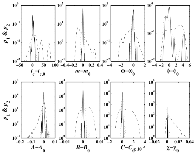
Figure 3: Probability density functions $p_{1}(x-x_{0})$ (continuous lines), $p_{2}(x-x_{0})$ (dashed lines), and $p^{*}_{1}(x-x_{0})$ (dotted lines) associated with a reference antibubble from 2000/08/09 to $t_{\rm{last}}={\rm{2003/08/15}}$ for the eight parameters deriving from the fits with the log-periodic formula (1). $p^{*}_{1}(x-x_{0})$ is modified from $p_{1}(x-x_{0})$ by using a more realistic noise process, as explained in the text.

Figure 3 plots the probability density functions (PDFs), $p_{1}(x-x_{0})$ (solid lines) and $p_{2}(x-x_{0})$ (dashed lines), of the difference between a given fit parameter $x$ and its reference value $x_{0}$, for the two classes associated with the antibubble that developed from 2000/08/09 to $t_{\rm{last}}={\rm{2003/08/15}}$. The index $1$ (respectively $2$) refers to Class I (respectively II). The variable $X$ stands for any of the parameters $t_{c}$, $m$, $\omega$, $\phi$, $A$, $B$, $C$, and $\chi$. The reference value $x_{0}$ is the value of the parameter obtained in the fit of the antibubble from 2000/08/09 to $t_{\rm{last}}={\rm{2003/08/15}}$ with the log-periodic formula. The differences between each pair of PDFs are significant: $p_{1}(x-x_{0})$ concentrates around $x-x_{0}=0$, as could be expected, while $p_{2}(x-x_{0})$ exhibits a much larger dispersion with much slower decaying tails.

In pattern recognition methods, it is necessary to define two types of errors that can occur in a classification scheme using a given fit parameter $x$. An error of type I occurs when the hypothesis, which is true, is rejected (a “false negative” in terms of null hypothesis testing). Errors of type I occur with a complementary cumulative probability $P_{1}(x)$ measured as the proportion of the objects in class I with a deviation $|X-x_{0}|$ greater than $|x-x_{0}|$:

$$P_{1}(x)=\lim_{N\to\infty}\frac{\sharp\{X:|X-x_{0}|>|x-x_{0}|~{}\&~{}X\in{\rm{I}}\}}{N}~{},$$ (4)

where $\sharp$ is the operator counting the number of elements in a given set. An error of type II occurs when an hypothesis, which is false, is accepted (a “false positive” or “false alarm” in terms of null hypothesis testing). Errors of type II occur with a cumulative probability $P_{2}(x)$ measured as the proportion of the objects in class II with the deviation $|X-x_{0}|$ smaller than $|x-x_{0}|$:

$$P_{2}(x)=\lim_{N\to\infty}\frac{\sharp\{X:|X-x_{0}|<|x-x_{0}|\}~{}\&~{}X\in{\rm{II}}\}}{N}~{}.$$ (5)

By definition, $\lim_{x\to x_{0}}P_{1}(x)=1$, $\lim_{x\to x_{0}}P_{2}(x)=0$, $\lim_{|x-x_{0}|\to\infty}P_{1}(x)=0$, and $\lim_{|x-x_{0}|\to\infty}P_{2}(x)=1$.

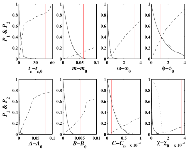
Figure 4: Probabilities $P_{1}(x)$ (continuous lines), $P^{*}_{1}(x)$ (dotted lines), and $P_{2}(x)$ (dashed lines) corresponding to the reference antibubble from 2000/08/09 to $t_{\rm{last}}={\rm{2001/08/15}}$ as functions of eight parameters derived from the fits with the log-periodic formula (1). The vertical lines indicate the realized values of $|x-x_{0}|$.

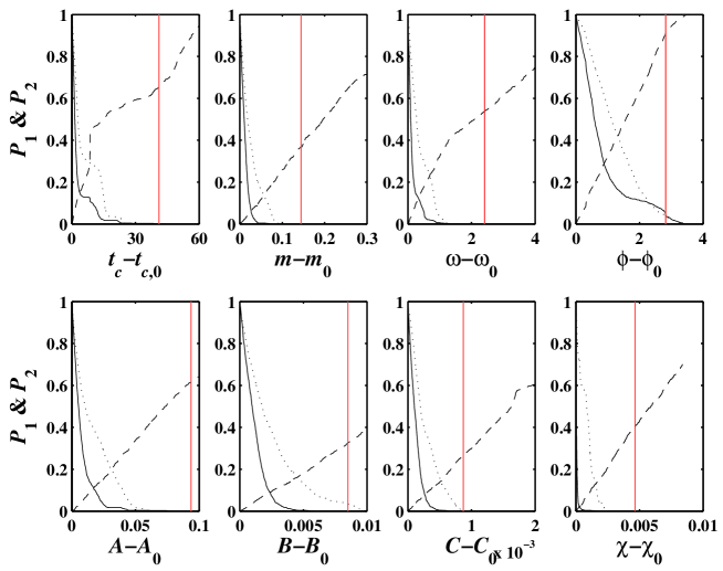
Figure 5: Same as Fig. 4 for $t_{\rm{last}}={\rm{2002/02/15}}$.

Figure 4 shows the probabilities $P_{1}(x)$ and $P_{2}(x)$ constructed by taking as the reference the antibubble on the S&P 500 from 2000/08/09 to $t_{\rm{last}}={\rm{2001/08/15}}$, for the seven fit parameters and for the r.m.s $\chi$. Figures 5 to 8 are the same for $t_{\rm{last}}={\rm{2002/02/15}}$, ${\rm{2002/08/15}}$, ${\rm{2003/02/15}}$, and ${\rm{2003/08/15}}$, respectively.

As seen in Figure 3, the PDF’s for Class I are extremely narrow. One may wonder if this is not due to our use of the GARCH process which gives a too conservative estimate of the noise impact. To test this possibility, we use another noise generating process. Rather than generating noise synthetically, we construct the time series of the residues $\epsilon(t)$ obtained from the log-periodic fit of the reference time series with the LPPL formulae. We then extract at random a six month segment of $\epsilon(t)$ which is the noise taken to decorate the extended series from $t_{\rm{last}}$ to $t_{\rm{last}}+6$ months for Class I objects. Having thus generated new objects of Class I, we calculate the new PDFs and the probabilities $P^{*}_{1}(x)$ defined as the proportion of the objects (with “residual” noise) in class I with a deviation $|X-x_{0}|$ greater than $|x-x_{0}|$. The new PDFs $p^{*}_{1}(x-x_{0})$ are shown as dotted line in Figure 3. The dependence of the corresponding $P^{*}_{1}(x)$ (defined as $P_{1}(x)$ but using $p^{*}_{1}(x-x_{0})$ instead of $p_{1}(x-x_{0})$) for the seven parameters and for the r.m.s. as a function of $|x-x_{0}|$ are shown as the dotted lines in Figs. 4 to 8. As expected, using past realized residuals gives slightly larger dispersions but the differences are not large. This confirms the large difference between objects in Class I and in Class II.

To qualify the continuation of the antibubble based on the measured value $x$ of one parameter, one would like to have both $P_{1}(x)$ large (above some threshold) and $P_{2}(x)$ small (below some threshold). The first condition ($P_{1}(x)$ sufficiently large) tells us that the realized deviation is well within the normal fluctuations of objects in Class I. The second condition ($P_{2}(x)$ sufficiently small) indicates that it is improbable to obtain such a value of $x$ if the price series was not an antibubble. These two conditions quantify how much deviation of $x$ from the reference value $x_{0}$ is tolerable to qualify the additional six month of data as a continuation of the antibubble.

In practice, using $t_{\rm{last}}={\rm{2003/08/15}}$, one has to wait an additional 6 month and analyze the realized time series as an object to be classified according to the above scheme. To test the sensitivity and reliability of this procedure, it is natural to turn to data in the past of $t_{\rm{last}}={\rm{2003/08/15}}$ to simulate how this method would have worked in this past. We will then turn below to examine the data posterior to $t_{\rm{last}}={\rm{2003/08/15}}$.

3.3 Ex-post tests

To assess the validity of the proposed method, we test it retroactively. The test consists in taking the price time series from 2000/08/09 to $t_{\rm{last}}$ as the reference and in applying the procedure described in section 3.2 for each $t_{\rm{last}}$, with $t_{\rm{last}}$ taking the values ${\rm{2001/08/15}}$, ${\rm{2002/02/15}}$, ${\rm{2002/08/15}}$, and ${\rm{2003/02/15}}$, with a time step of six months. We use the realized values of the fitted parameters obtained for the time series extending to $t_{\rm{last}}+6$ months to obtain the two probabilities $P_{1}$ and $P_{2}$. The realized values of $P_{1}$, $P_{1}^{*}$ and $P_{2}$ are listed in Table 1. The realized values of the fit parameters for the time series extending to $t_{\rm{last}}+6$ months are indicated by the vertical line in Figs. 4 to 8.

The rather poor results (small $P_{1}$’s, $P_{1}^{*}$’s and large $P_{2}$’s) for the two earlier times $t_{\rm{last}}={\rm{2001/08/15}}$ and $t_{\rm{last}}={\rm{2002/02/15}}$ can probably be attributed to the fact that the log-periodic structure was not yet sufficiently developed and was dominated by noise. A large $P_{2}$ in particular means that the six-month extension from $t_{\rm{last}}$ to $t_{\rm{last}}+6$ months had similarity with a random walk. For the two later times $t_{\rm{last}}={\rm{2002/08/15}}$ and $t_{\rm{last}}={\rm{2003/02/15}}$, we observe often large $P_{1}$’s and small $P_{2}$’s, suggesting that the antibubble has continued to develop. We should also stress that all parameters are not equivalent for the decision process. For instance, the r.m.s. of fit residuals is almost insensitive to the phase $\phi$, which explains why the values of $P_{1}$ and $P_{2}$ are completely uninformative for the phase.

3.4 Impact of past regime switching: contaminated reference

The previous tests have been performed with the hypothesis that the antibubble have been genuinely continuing until $t_{\rm{last}}$. This condition has allowed us to take the parameters of the fits of the time series up to $t_{\rm{last}}$ as references. But what about the possibility that the price time series has already switched to a random walk? It could be the case that we may incorrectly believe in the antibubble continuation until $t_{\rm{last}}$ while in fact a part of the past time series is already in the random walk regime. The reference values of the fitted parameters would then be incorrect, leading to possible distortions in the calculation of $P_{1}$ and $P_{2}$.

We thus also need to take into account the fact that the regime switch may have happened in the past, to quantify what is its effect in qualifying its future. To address this question, we replace the data of the last six months of the reference series ending at $t_{\rm{last}}$ by a random walk with time steps equal to the historical volatility. Specifically, from the beginning of the time series to $t_{\rm{last}}-6$ months, the time series is the S&P 500 data. From $t_{\rm{last}}-6$ months to $t_{\rm{last}}$, we extend the S&P 500 data by generating a random walk. The resulting time series ending at $t_{\rm{last}}$ is then taken at the believe-to-be-true antibubble to which we apply the above procedure described in section 3.2.

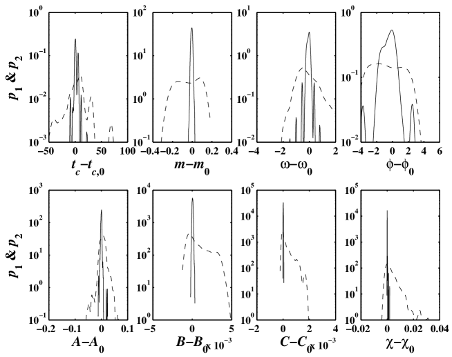
Figure 9: Probability density functions $p_{1}(x-x_{0})$ (continuous lines) and $p_{2}(x-x_{0})$ (dashed lines) associated with a contaminated reference antibubble from 2000/08/09 to $t_{\rm{last}}={\rm{2003/08/15}}$ for the eight parameters derived from the fits with the log-periodic formula (1). See Sec. 3.4 for details.

The tests are performed for $t_{\rm{last}}={\rm{2003/02/15}}$ and ${\rm{2003/08/15}}$. The results are given in Figs. 9 to 11, where the vertical lines indicate the values of the realized $|x-x_{0}|$ for the time series ending at $t_{\rm{last}}+6$ months. In Fig. 9, one observes a broadening of $p_{1}$ as can be expected.

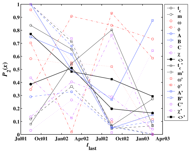
Figure 12: Probability $P_{2}(x)$ as a function of $t_{\rm{last}}$ for the different parameters. The non-prime parameters are defined in Sec. 3.2 and correspond to the uncontaminated reference case. The primed parameters are defined in Sec. 3.4 and correspond to the contaminated reference case. The thick lines with close circles and squares give the average over the eight parameters for the two types of $P_{2}$ (uncontaminated and contaminated respectively).

Fig. 12 shows $P_{2}$ as a function of $t_{\rm{last}}$ for the uncontaminated cases (circles) studied in Sec. 3.2 and for the contaminated cases (squares) studied in this section for each of the 8 parameters. The adjective uncontaminated (respectively contaminated) refers to taking the true time series up to $t_{\rm{last}}$ (respectively to replacing the true time series by a random walk in the interval from $t_{\rm{last}}-6$ months to $t_{\rm{last}}$). The overall picture is that the squares for the contaminated case tend to spread more uniformly in $[0,1]$ while the uncontaminated case becomes more concentrated towards smaller values of $P_{2}$ for the last three $t_{\rm last}$. The means of $P_{2}$ for the uncontaminated (respectively contaminated) cases are shown in thick lines with closed circles and squares respectively. One can observe that the $P_{2}$’s for the contaminated case are significantly larger than for the uncontaminated case, suggesting that it may be possible to distinguish between them.

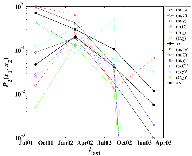
Figure 13: Combined probability $P_{2}(x_{1},x_{2})$ as a function of $t_{\rm{last}}$ for both uncontaminated (circles) and contaminated (squares) cases. Pairs $(x_{1},x_{2})$ are formed by taking $x_{1}$ and $x_{2}$ in the set $\{m$, $\omega$, $C$, $\chi\}$. The thick lines with close circles and squares give the average over the eight parameters for the two types of $P_{2}$ (uncontaminated and contaminated respectively).

Fig. 13 plots the product of two $P_{2}$’s associated with two parameters chosen from the set $\{m$, $\omega$, $C$, $\chi\}$, both for uncontaminated (circles) and contaminated (squares) cases. We denote $P_{2}(x_{1},x_{2})$ the product of the two $P_{2}$’s associated with the parameters $x_{1}$ and $x_{2}$. We also perform the averages over all pairs of $P_{2}(x_{1},x_{2})$, for the uncontaminated and for the contaminated cases, which are shown with filled circles and squares respectively. The construction of $P_{2}(x_{1},x_{2})$ constitutes one step in the direction of a decision for the qualification or disqualification of the antibubble which should be ideally performed on the basis of the full multivariate distributions over all parameters simultaneously. One can observe significantly larger $P_{2}(x_{1},x_{2})$’s for the uncontaminated cases compared with the contaminated cases. The fact that $P_{2}(x_{1},x_{2})$ tends to decrease for the last three points can be interpreted as follows: the data has accumulated more so that the log-periodic structure has become more developed, which constrains more the fits. As a consequence, it is thus less probable to misinterpret a random walk for a genuine LPPL antibubble between $t_{\rm{last}}$ and $t_{\rm{last}}+6$ months. Notice also the slower decay of $P_{2}(x_{1},x_{2})$ for the last two points for the uncontaminated cases compared with the contaminated cases.

3.5 Testing the end of the antibubble: formulation and implementation

As an empirical implementation of our detection method, we propose the following test for the possible end of the antibubble, based on selected scenarios for the future. To illustrate the method, we take the date of 2003/08/15 as the end of the known time series, and then project several possible scenarios over the following six months. For each scenario, the characteristic probabilities $P_{1}$ and $P_{2}$ are calculated and used to characterize the two possible outcomes: (i) the antibubble continues or (ii) the antibubble has ended. We then apply this procedure to the realized data from 2003/08/15 to 2004/02/15 (2003/08/15 $+$ six months). In the first version of this paper available in August 2003 (v.1 at http://arxiv.org/abs/cond-mat/0310092), we performed the first part in real time and out-of-sample. The time elapsed since allows us to describe the conclusion of this test on the realized data.

3.5.1 Synthetic scenarios

Let us thus consider 2003/08/15 (for which the S&P 500 was slightly below 1000) as the date from which we project scenarios to test for the continuation or ending of the antibubble. We extend the price time series beyond 2003/08/15 by constructing seven different scenarios of the future S&P 500 evolution for the next six months:

• a random walk taking the S&P 500 to the value 1200;

• a random walk taking the S&P 500 to 1100;

• a random walk taking the S&P 500 to 1000;

• a random walk taking the S&P 500 to 900;

• a random walk taking the S&P 500 to 800;

• a continuation of the antibubble with noise obtained by a GARCH process described in Sec. 3.2 (Class I and $P_{1}$); and

• a continuation of the antibubble with noise obtained by drawing at random the residuals over six previous months as in Sec. 3.2 (Class I and $P^{*}_{1}$).

We have generated 424 realizations for each of these seven scenarios ending at 2004/02/15 (2003/08/15 plus 6 months). Each realization, which has been fitted by the LPPL formula (1), yields 7 parameters and the r.m.s. For each realization, the two probabilities $P_{1}$ and $P_{2}$ defined in (4) and (5) are obtained for the seven parameters, from which their average and standard deviations are determined. The results are shown in Table 2. The most striking observation is that $P_{1}$ is small (respectively large) for the five random walk scenarios (respectively for the continuation of the antibubble), while $P_{2}$ is large (respectively small) for the five random walk scenarios (respectively for the continuation of the antibubble). As expected, for the five random walk scenarios, $P_{1}$ increases and $P_{2}$ decreases with decreasing ending value of the synthetic values. These results suggest that one should be able to distinguish clearly the continuation of the antibubble from a regime switch to a random walk beyond 2003/08/15. However, one should keep in mind that the real future evolution might be more complicated than a random walk trajectory with consequences for the test which are difficult to foresee.

The fact that $P_{1}$ is so small for the random walk scenarios (i)-(v) and quite large for the continuation of the antibubble scenarios (vi) and (vii) tells us something important. Recall that $P_{1}$ quantifies the probability that the deviations on the LPPL parameters is larger in a true LPPL antibubble continuation than those obtained from the scenarios. Small $P_{1}$’s for the random walk scenarios (i)-(v) means that, conditioned on the fact that we believe (erroneously) that the scenarios (i)-(v) are genuine LPPL structures, essentially any random realization decorating a true LPPL structure would continue to qualify as a genuine LPPL structure. In other words, $P_{1}$ can be interpreted as the probability of existence of the LPPL antibubble. It is very small for the random walk scenarios (i)-(v) and quite large for the continuation of the antibubble scenarios (vi) and (vii). Reciprocally, the fact that $P_{2}$ is so large for the random walk scenarios (i)-(v) is in line with the fact that LPPL fits give large errors for these scenarios and thus, conditioned on the fact that these scenarios are believed a priori to be genuine LPPL antibubbles, it is very probable that random walk realizations would give similar or even better LPPL fits. In other words, what this test tells us is that, starting with a bad fit, additional noise can give similar or better fits. In contrast, the low value of $P_{2}$ for the continuation of the antibubble scenario (vi) and (vii) means that random walk extensions are very unlikely to give qualities of fits similar to those obtained on average for these scenarios (vi) and (vii). In sum, the small $P_{1}$ and large $P_{2}$ found for the random walk scenarios (i)-(v) are good signals of the end of the LPPL antibubble. In contrast, the large $P_{1}$ and small $P_{2}$ found for the continuation scenarios (vi) and (vii) are good signals of the continuation of the LPPL antibubble.

Thus, we conclude that, given the present price pattern, there is only a small probability of making an error in diagnosis: (a) if we obtain a small $P_{1}$ and a large $P_{2}$ in the realized six months from 2003/08/15 to 2004/02/15, we will conclude that the antibububble has ended; (b) in contrast, if we obtain a large $P_{1}$ and a small $P_{2}$, we will conclude that the antibubble continues.

3.5.2 Realized probabilities and apparent end of the US antibubble

Let us apply the test just described to the realized data from 2003/08/15 to 2004/02/15. In the first version of our paper presented in Sec. 3.5.1, we could not conclude that the antibubble had ended yet and suggested that we would be able to decide when the data till Feb 2004 would become available. Here we complete this test.

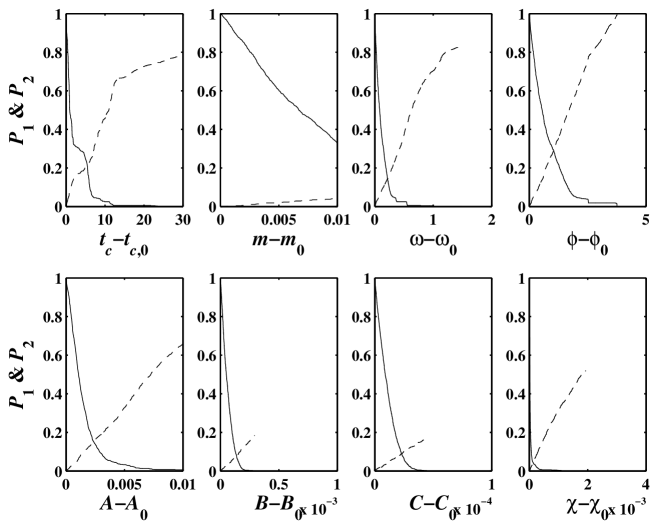
Figure 11: Same as Fig. 10 for $t_{\rm{last}}={\rm{2003/08/15}}$.

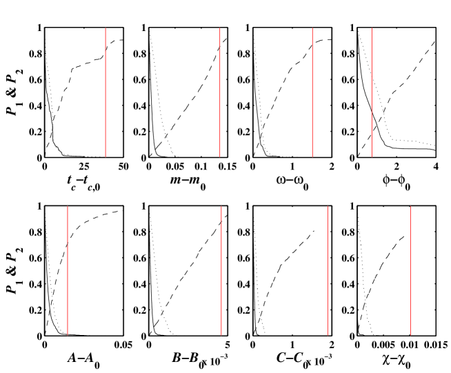
Figure 14: Probabilities $P_{1}(x)$ (continuous lines), $P^{*}_{1}(x)$ (dotted lines), and $P_{2}(x)$ (dashed lines) corresponding to the reference antibubble from 2000/08/09 to $t_{\rm{last}}={\rm{2004/02/15}}$ as functions of eight parameters derived from the fits with the log-periodic formula (1). The vertical lines indicate the realized values of $|x-x_{0}|$.

For this, Figure 14 shows the probabilities $P_{1}$ (continuous lines), $P_{1}^{*}$ (dotted lines), and $P_{2}$ (dashed lines) corresponding to the reference antibubble from 2000/08/09 to 2003/08/15 as functions of eight parameters derived from the fits with the first-order log-periodic formula, which was shown in Fig. 11. The vertical lines indicate the realized values of $|x-x_{0}|$, where $x_{0}$ is the reference value. One can see that the $P_{1}$’s are very small and the $P_{2}$’s are very large for all parameters but the phase $\phi$, which was previously shown to be irrelevant anyway. The small values of $P_{1}$ and large values of $P_{2}$ indicate that the antibubble in the USA has apparently ended.

3.6 S&P 500 in other currencies

In the previous tests, the S&P 500 index was valued in the local currency, the US dollar. In a sense, this corresponds to making a joint analysis of the behavior of the S&P 500 index and of the US$. One can worry about the possibility that something has affected the US$ so that the behavior of the S&P 500 index may have been distorted when viewed from the US$ lens. This question boils down in fact to the following: who are the investors moving the market and what is the correct reference currency? In [22], we have found strong evidence of fueling of the 2000 new economy bubble by foreign capital inflow. More generally, foreigners constitute a growing part of the investment pool [23] influencing US markets in particular with the recycling of surpluses from Asian countries, as their moves in and out of the market are more frequent and volatile than the major investing US funds, due to a large current account deficit that must be financed, fear of a weakening dollar, the impact of a rising or decreasing dollar, and so on. Since the burst of the new economy bubble in 2000, the Federal Reserve has decreased its leading short term interest rate in a series of steps (see [24] for a detailed analysis of this Fed policy and its relationship with the US stock market); it has been argued by many observers that these moves may have artificially distorted the available liquidity in addition to direct monetary interventions, amounting to an effective inflation in dollar terms, hence its depreciation, with observable consequences in the real estate boom [25] (the rising price of real estate is the same as the decrease in the value of the dollar with respect to these assets). This suggests to deconvolve the time evolution of the US stock market from the US$, which amounts to taking the view point of either a prudent investor comparing stock with a supposedly risk haven such a gold or the view point of a foreign investor by converting the market price in euro, British pound or Yen, for instance.

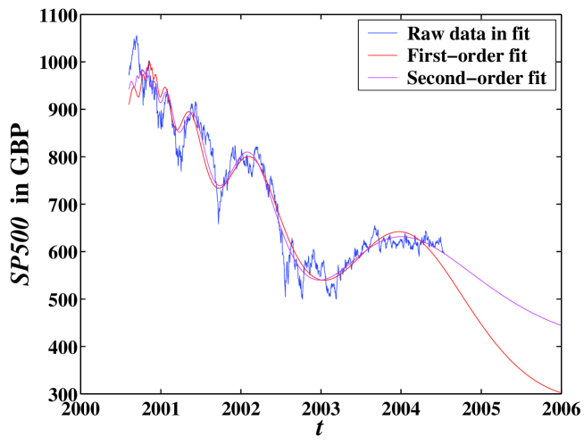
Figure 15: The S&P 500 index denominated in GBP from 2000/08/09 to 2004/07/16 and its fits using the first-order and second-order Landau formulas. The values of the fit parameters are listed in Table 3. The fits are extrapolated to the end of 2005.

We have fitted the S&P 500 index denominated in British pound, Canadian dollar, euro, gold fixes FM, Hong Kong dollar, Japanese Yen, XAG, as well as US dollar for comparison, from 2000/08/09 to 2004/07/16, using the first-order and second-order Landau formulae. We find that the fits for Japanese Yen and XAG are even worse than that for the US dollar, while Canadian dollar, gold fixes FM, and Hong-Kong dollar give similar results compared with the US dollar. Interestingly, the analyses using the British pound and the euro give much more convincing fits. A typical plot is illustrated in Fig. 15 for the US market expressed in British pounds. The parameter values of the fitting to S&P 500 denominated in different currencies (British pound, euro, gold fixes FM, and US dollar) are listed in Table 3. Given the quality of such fits, our previous methodology (not shown for brevity) concludes that the antibubble continues from the European investor view point.

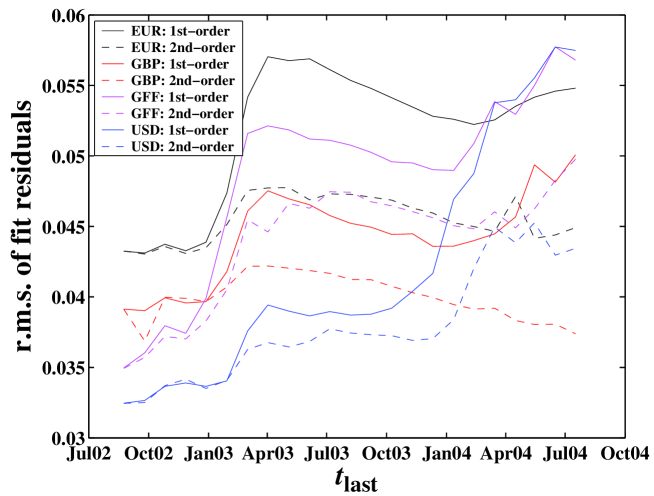
Figure 16: Evolution of the RMS of residuals of the fit of the S&P500 index expressed in four different currencies with the first-order and second-order Landau formulae.

The parameters shown in Table 3 suggest that the crossover from the first-order to the second-order regime has occurred, which means a significant change in the values of the angular log-frequency during the development of the antibubble. We note in particular a quite significant difference of RMSE’s between the two fits, as also shown in Fig. 16. Figure 16 shows the evolution of the r.m.s. (root-mean-square, an inverse measure of the quality of the fits) of the fit residuals of the respective fits. In general, the discrepancy between the two fits (with the first-order and second-order formulae) of a given currency increases when more data are included. The separations between the dashed versus corresponding continuous lines illustrate the crossover from the first order to the second order.

Figure 16 identifies very clearly a change of regime around February 2003, materialized by the jump in r.m.s. in all fits and, at the same time, the sudden increase of the r.m.s. of the first-order formula compared with the r.m.s. of the second-order formula. The same phenomenon is documented above for the S&P 500 in US dollar. Beyond the quality and predictive power of the proposed fits, we would like to stress the importance of identifying “regime switches”. Roughly speaking, Fig. 16 shows that the r.m.s. of the fit residuals for foreign currencies of the second-order Landau formula keep decreasing as a function of time (the quality of the fits increase), in contrast with those of the first-order formula. This confirms the visual impression that the second-order Landau fits capture very well the LPPL oscillations when compared with the first-order fits, as exemplified in Fig. 15.

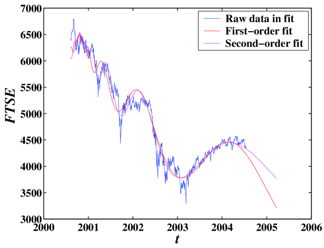
Figure 17: The FTSE index (in british pounds) from 2000/08/09 to 2004/07/16 and its fits using the first-order and second-order Landau formulas. The fits are extrapolated to the beginning of 2005.

These analyses imply that the S&P 500 antibubble started in mid-2000 is still alive, when denominated in European currencies. A natural question is then to ask if the antibubble in the European stock markets is still continuing since those stocks are traded directly in EUR and in GBP. We have fitted three major indexes in Europe, that is, CAC 40 of France, DAX of Germany, and FTSE 100 of the United Kingdom. The results are very similar to each other. We thus take FTSE as an example shown in Figure 17. This figure presents the FTSE of the United Kingdom from 2000/08/09 to 2004/07/16 and its fits using the first-order and second-order Landau formulas. We see that the antibubble is right on track in these stock markets in Europe. The tentative conclusion of this study is that the strong impact of the intervention of the US Federal Reserve has perturbed the fingerprints of the antibubble of the US stock markets when viewed in local currencies, while it is possible in reality that the herding bearish-bullish oscillations are still present but are hidden by the distorting feedback actions of the Federal Reserve and the perturbed behavior of the US$. Correcting for this possible bias by taking the view point of an European investor, we conclude that the antibubble may well be continuing. Similar conclusions hold when taking gold as the reference unit to express the value of the US stock markets (see [2]).

4 Concluding remarks

First, we have presented a general methodology to test for a cross-over or a shift in log-periodicity. Second, we have developed a battery of tests to detect a possible end of the antibubble. Our conclusion is that the antibubble was still probably alive in August 2003 but has ended since in the USA (i.e., when viewed from the view point of a US investor valuing in US dollars). More generally, our tests provide new quantitative measures to diagnose the end of an antibubble and this will be useful for future applications. We find that such diagnostic is not instantaneous and requires probably three to six months within the new regime before assessing its existence with confidence. We have also found that the antibubble is still continuing when viewed from the point of view of a European investor or alternatively from an investor valuing the US stock market with respect to gold. We attribute the discrepancy between our two conclusions to the depreciation of the US dollar in the last two years, which is linked to the Federal Reserve interest rate and monetary policy.

This present paper follows several others [1, 4, 6, 18] which were nucleated by noticing a similarity between the Nikkei antibubble that started in January 1990 and the present US antibubble that started in August 2000, when shifted approximately by 11 years. We conclude with a word of caution concerning this similitude between the two time series: the noted similarity should not lead to the belief that the S&P 500 index is bound to follow blindly in the future the path suggested by the Nikkei. In contrast with chartism or technical analysis, our approach is to develop a scientific understanding of these bubble-antibubble phases. The similitude between the Nikkei and US markets is part of the search for “universal” properties, that allow us to establish a theory (in short, a theory is a story of repeatable/reproducible occurrences). Using this theory then allows us to describe idiosyncratic behaviors, that is, deviations from one case to another, or in other words, the parts of the evolutions that are not universal. This is what should give us an hedge for predictions. This is why we have emphasized in previous works the similitude between the shifted Nikkei and the US stock markets [6].

However, after three-year evolution of the S&P 500 antibubble, the discrepancy between the Nikkei and S&P 500 antibubbles became detectable. The qualitative analogy is still there but, quantitatively, there are differences. Technically, after two years and a half after the top in December 31, 1989, we find that the Nikkei has started to shift to another antibubble regime while no such shift was detectable after the same time span since the start of the antibubble in the US. Only when using data up to the summer of 2003, we find suggestions of such a change of regime. In addition, the US markets have been characterized by much stronger crashes and rallies, modelled by the so-called zero-phase Weierstrass-type functions [18]. These two facts suggest that the herding forces are even stronger in the US and that investors react even more on hair-trigger to any “news.” The similarities between the shifted Nikkei and the S&P 500 are qualitative: bubble preceding antibubble, strong speculation and herding, similar fear and herding in the antibubble regime, some problems with bad loans or bad accounting, strong commitment from the central banks and governments to provide liquidity and cash… But there are differences and these differences can be detected already after three-year evolution of the S&P 500 antibubble and even more after four years.

There are also interesting structural differences in the origin of the bubbles that preceded their antibubbles. Japan was (and still is) a surplus country, whose strong positive balance of payment led to “high-powered” money being poured in the country. This in turn powered speculation and price appreciation to sky-rocketing levels. The so-called bad loans dragging down the Japanese recovery came from this epoch when the high-powered money input was used by banks to provide loans amplified by the multiplier effect for purchases at prices often substantially larger than the real value. In contrast, the USA has become in the last decade a deficit country, accumulating an increasingly large negative balance of payment with the rest of the world. The bubble that developed in the 1990s was fuelled indirectly by the surplus dollars accumulated by foreign countries which were re-injected in the US in the hope of getting a reasonable return while avoiding the risk of appreciation of their own currencies [22]. The bubble had also a very strong endogenous component of self-reinforcing belief in a “new economy,” a characteristic that could be matched to the faith in the Japanese miracle underlying the Japanese bubble. Thus both the Japanese and USA markets are strongly linked to the behavior of international investors and central bankers and to the belief and confidence of investors, but the specifics of the herding and over-optimism have sometimes different origins. It remains to be seen if this will lead to appreciable differences in the evolution of the two antibubbles.

Acknowledgments We are grateful to V.F. Pisarenko for useful remarks on the manuscript. We also thank Harald W. Ade, Chris Couteau, Ronald Guy, and John Hunter for helpful interactions.

Table 1: Results of ex-post tests of the end of an antibubble described in section 3.3 with two classes of synthetic time series.

	$t_{\rm{last}}$	$t_{c}$	$m$	$\omega$	$\phi$	$A$	$B$	$C$	$\chi$
$P_{1}:$	2001/08/15	0.000	0.014	0.000	0.418	0.000	0.000	0.585	0.000
	2002/02/15	0.001	0.000	0.000	0.053	0.000	0.000	0.000	0.000
	2002/08/15	0.701	0.051	0.169	0.314	0.161	0.077	0.011	0.000
	2003/02/15	0.139	0.945	0.011	0.081	0.065	0.969	0.894	0.000
$P_{2}:$	2001/08/15	0.838	0.119	0.582	0.345	0.749	0.290	0.031	0.136
	2002/02/15	0.655	0.369	0.537	0.908	0.616	0.328	0.265	0.404
	2002/08/15	0.067	0.066	0.096	0.838	0.050	0.057	0.115	0.289
	2003/02/15	0.273	0.002	0.116	0.733	0.152	0.002	0.000	0.041
$P_{1}^{*}$:	2001/08/15	0.000	0.018	0.000	0.530	0.000	0.000	0.662	0.000
	2002/02/15	0.000	0.000	0.000	0.347	0.000	0.033	0.000	0.000
	2002/08/15	0.631	0.297	0.339	0.145	0.461	0.351	0.085	0.000
	2003/02/15	0.236	0.982	0.030	0.080	0.070	0.993	0.943	0.001

Table 2: Probabilities for the two types of errors concerning seven scenarios extrapolating the S&P 500 index over six months from 2003/08/15 in the future. The numbers in the parentheses stand for the standard deviations. See section 3.5.1 for a description of the testing procedure.

	Scenario	$~{}~{}t_{c}$	$~{}~{}m$	$~{}~{}\omega$	$~{}~{}\phi$	$~{}~{}A$	$~{}~{}B$	$~{}~{}C$	$~{}~{}\chi$
$P_{1}:$	i	$0.000(1)$	$0.001(6)$	$0.000(0)$	$0.057(64)$	$0.000(0)$	$0.172(216)$	$0.000(0)$	$0.000(0)$
	ii	$0.000(3)$	$0.000(0)$	$0.000(0)$	$0.093(118)$	$0.007(35)$	$0.000(0)$	$0.000(0)$	$0.000(0)$
	iii	$0.025(58)$	$0.000(0)$	$0.002(3)$	$0.271(242)$	$0.086(141)$	$0.000(0)$	$0.000(0)$	$0.004(2)$
	iv	$0.216(105)$	$0.002(3)$	$0.057(81)$	$0.066(74)$	$0.058(72)$	$0.002(3)$	$0.019(86)$	$0.009(1)$
	v	$0.063(70)$	$0.000(1)$	$0.008(14)$	$0.100(115)$	$0.309(218)$	$0.002(27)$	$0.000(2)$	$0.000(0)$
	vi	$0.490(283)$	$0.508(294)$	$0.485(277)$	$0.484(280)$	$0.495(290)$	$0.508(294)$	$0.511(298)$	$0.495(284)$
	vii	$0.436(261)$	$0.215(303)$	$0.378(281)$	$0.386(278)$	$0.305(250)$	$0.216(299)$	$0.213(286)$	$0.024(82)$
$P_{2}:$	i	$0.955(44)$	$0.269(37)$	$0.917(34)$	$0.814(215)$	$0.982(4)$	$0.061(33)$	$0.728(31)$	$0.965(3)$
	ii	$0.847(67)$	$0.714(62)$	$0.818(57)$	$0.675(212)$	$0.843(86)$	$0.712(66)$	$0.898(32)$	$0.805(6)$
	iii	$0.581(144)$	$0.665(68)$	$0.601(101)$	$0.351(250)$	$0.467(197)$	$0.792(80)$	$0.697(30)$	$0.239(26)$
	iv	$0.243(99)$	$0.184(20)$	$0.251(66)$	$0.701(262)$	$0.442(90)$	$0.232(28)$	$0.096(17)$	$0.153(31)$
	v	$0.431(138)$	$0.420(62)$	$0.474(97)$	$0.726(247)$	$0.218(203)$	$0.300(49)$	$0.374(23)$	$0.771(21)$
	vi	$0.131(137)$	$0.026(28)$	$0.075(84)$	$0.191(236)$	$0.129(144)$	$0.027(30)$	$0.025(21)$	$0.014(36)$
	vii	$0.150(139)$	$0.084(65)$	$0.106(92)$	$0.258(256)$	$0.223(178)$	$0.085(66)$	$0.065(45)$	$0.195(99)$

Table 3: Parameter values of the fitting to S&P 500 denominated in different currencies (British pound, euro, gold fixes FM, and US dollar) using the first-order and second-order Landau formulae. The data are from 2000/08/09 to 2004/07/16. The superscripts $1$ and $2$ stand for the order of the Landau formula used in fitting.

Currency	$t_{c}$	$m$	$\omega$	$\phi$	$\Delta_{t}$	$\Delta_{\omega}$	$A$	$B$	$C$	$\chi$
EUR1	2000/10/31	0.84	6.56	3.48			7.40	-1.95E-3	5.46E-4	0.0548
EUR2	2000/10/05	0.90	9.23	0.00	3343	-45	7.40	-1.29E-3	4.44E-4	0.0449
GBP1	2000/10/07	0.78	7.07	0.02			6.91	-2.66E-3	7.97E-4	0.0501
GBP2	2000/07/30	0.99	11.92	4.05	2689	-49	6.92	-6.20E-4	-2.07E-4	0.0374
GFF1	2000/09/17	0.91	5.27	2.70			1.69	-1.26E-3	-3.30E-4	0.0568
GFF2	2000/10/18	0.90	8.65	0.72	5232	-78	1.69	-1.49E-3	-4.06E-4	0.0498
USD1	2000/09/05	0.72	5.63	0.32			7.25	-2.55E-3	-1.20E-3	0.0575
USD2	2000/09/08	0.63	11.01	2.12	6902	-64	7.29	-5.87E-3	2.48E-3	0.0434

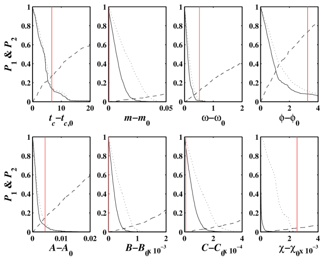
Figure 7: Same as Fig. 4 for $t_{\rm{last}}={\rm{2003/02/15}}$.

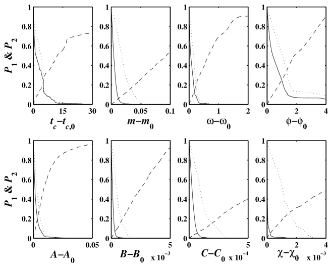
Figure 8: Same as Fig. 4 for $t_{\rm{last}}={\rm{2003/08/15}}$.

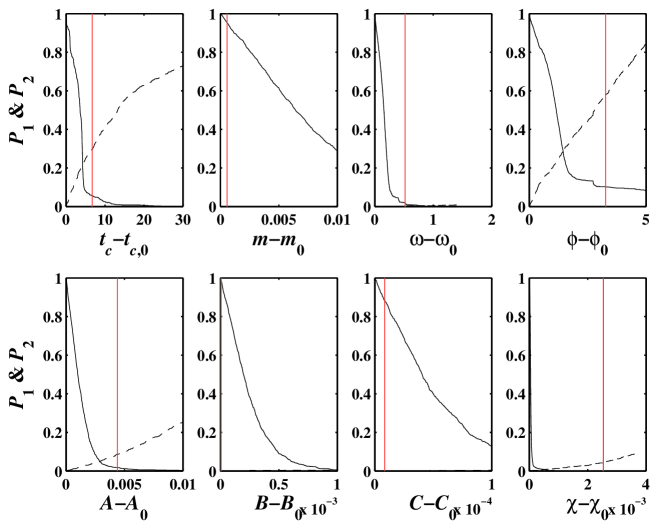
Figure 10: Probabilities $P_{1}(x)$ (continuous lines) and $P_{2}(x)$ (dashed lines) corresponding to a contaminated reference antibubble from 2000/08/09 to $t_{\rm{last}}={\rm{2001/08/15}}$ as functions of the eight parameters derived from the fits with the log-periodic formula (1). The vertical lines indicate the realized values of $|x-x_{0}|$.

References

- [1] D. Sornette and W.-X. Zhou, The US 2000-2002 Market Descent: How Much Longer and Deeper? Quantitative Finance 2 (2002) 468-481.
- [2]
- [3] A. Johansen and D. Sornette, Financial “antibubbles”: Log-periodicity in Gold and Nikkei collapses, Int. J. Mod. Phys. C 10 (1999) 563-575.
- [4] W.-X. Zhou and D. Sornette, Evidence of a worldwide stock market log-periodic antibubble since mid-2000, Physica A 330 (2003) 543-583.
- [5] A. Johansen, An alternative view, Quantitative Finance 3 (2003) C6-C7.
- [6] D. Sornette and W.-X. Zhou, The US 2000-2003 market descent: clarifications, Quantitative Finance 3 (2003) C39-C41.
- [7] P. Gnacinski and D. Makowiec, Another type of log-periodic oscillations on Polish stock market, Physica A, in press, preprint at cond-mat/0307323.
- [8] A. Johansen and D. Sornette, Evaluation of the quantitative prediction of a trend reversal on the Japanese stock market in 1999, Int. J. Mod. Phys. C 11 (2000) 359-364.
- [9] D. Sornette, Why Stock Markets Crash (Critical Events in Complex Financial Systems), Princeton University Press, Princeton, NJ, 2003.
- [10] D. Sornette, Critical market crashes, Physics Reports 378 (2003) 1-98.
- [11] A. Johansen and D. Sornette, Endogenous versus Exogenous Crashes in Financial Markets, in press in “Contemporary Issues in International Finance” (Nova Science Publishers, 2004) preprint at cond-mat/0210509.
- [12] D. Sornette and W.-X. Zhou, Predictability of Large Future Changes in Complex Systems, in press in the International Journal of Forecasting (2004) (http://arXiv.org/abs/cond-mat/0304601)
- [13] B.M. Roehner, Determining bottom price-levels after a speculative peak, Eur. Phys. J. B 17 (2000) 341-345.
- [14] B.M. Roehner, Identifying the bottom line after a stock market crash, Iny. J. Mod. Phys. C 11 (2000) 91-100.
- [15] K. Ide and D. Sornette, Oscillatory finite-time singularities in finance, population and rupture, Physica A 307 (2002) 63-106.
- [16] D. Sornette and K. Ide, Theory of self-similar oscillatory finite-time singularities in finance, population and rupture, Int. J. Mod. Phys. C 14 (2002) 267-275.
- [17] D. Sornette and A. Johansen, Large financial crashes, Physica A 245 (1997) 411-422.
- [18] W.-X. Zhou and D. Sornette, Renormalization group analysis of the 2000-2002 antibubble in the US S&P 500 index: Explanation of the hierarchy of five crashes and prediction, Physica A 330 (2003) 584-604.
- [19] D. Sornette, Y. Malevergne and J.-F. Muzy, What causes crashes? Risk 16 (2003) 67-71.
- [20] I. M. Gelfand, S. A. Guberman, V. I. Keilis-Borok, L. Knopoff, F. Press, E. Ya. Ranzman, I. M. Rotwain and A. M. Sadovsky, Pattern-recognition applied to earthquake epicenters in california, Phys. Earth Planet In. 11 (1976) 227-283.
- [21] V.I. Keilis-Borok and A.A. Soloviev, eds., Nonlinear Dynamics of the Lithosphere and Earthquake Prediction (Springer, Heidelberg, 2003).
- [22] D. Sornette and W.-X. Zhou, Evidence of fueling of the 2000 new economy bubble by foreign capital inflow: Implications for the future of the US economy and its stock market, Physica A 332 (2004) 412-440.
- [23] R.U.I. Albuquerque, N. Loayza and L. Serven, World Market Integration Through the Lens of Foreign Direct Investors, working paper (2003)
- [24] W.-X. Zhou and D. Sornette, Causal Slaving of the U.S. Treasury Bond Yield Antibubble by the Stock Market Antibubble of August 2000, Physica A 337 (2004) 586-608.
- [25] W.-X. Zhou and D. Sornette, 2000-2003 Real Estate Bubble in the UK but not in the USA, Physica A 329 (2003) 249-263.