Langevin vortex dynamics for a layered superconductor in the lowest Landau level approximation

Abstract

We have numerically investigated the dynamics of vortices in a clean layered superconductor placed in a perpendicular magnetic field. We describe the energetics using a Ginzburg-Landau free energy functional in the lowest Landau level approximation. The dynamics are determined using the time-dependent Ginzburg-Landau approximation, and thermal fluctuations are incorporated via a Langevin term. The c-axis conductivity at nonzero frequencies, as calculated from the Kubo formalism, shows a strong but not divergent increase as the melting temperature $T_{M}$ is approached from above, followed by an apparently discontinuous drop at the vortex lattice freezing temperature. The discontinuity is consistent with the occurrence of a first-order freezing. The calculated equilibrium properties agree with previous Monte Carlo studies using the same Hamiltonian. We briefly discuss the possibility of detecting this fluctuation conductivity experimentally.

I Introduction

Vortices in the mixed state of a clean type-II superconductor are believed to break the translational symmetry and form a triangular Abrikosov lattice for magnetic field $B$ exceeding the lower critical field $H_{c1}$. At a sufficiently high temperature $T$, thermal fluctuations are expected to melt this lattice and restore the translational symmetry through a solid-liquid phase transition. However, in most low-$T_{c}$ superconductors, this melting occurs near the upper critical field $H_{c2}$, and is thus difficult to distinguish from the usual superconducting-normal transition. In the high-T_c cuprates, however, this melting transition is typically well separated from $H_{c2}$.

Many experiments suggest that this solid-liquid phase transition is first order. For example, the resistivity of untwinned single crystals of YBa₂Cu₃O_7-δ (YBCO) drops sharply at a temperature $T_{M}$ well below the $H_{c2}(T)$ line. kwok1 This temperature also coincides with a discontinuous jump in the magnetization. kwok2 ; liang Most distinctively, both a latent heat and a specific heat discontinuity have been observed at the transition. These signatures have been seen in untwinned single crystals of YBCO for magnetic fields both parallel and perpendicular to the c-axis. kwok3

The first order nature of the transition is supported by a number of theoretical models. sasik1 ; sasik1a ; hu ; nordborg ; moore At least at high fields, this transition is thought to represent a simultaneous melting of the vortex lattice in the ab-plane and decoupling of the vortex “pancakes” in different layers. For example, numerical studies of layered superconductors, using Monte Carlo methods applied to a model Hamiltonian in the lowest Landau level (LLL) approximation, suggest a simultaneous melting and decoupling transition.sasik1 ; sasik1a ; hu A similar conclusion is also suggested by studies of melting using an analogy with a $2$D Bose system.nordborg On the other hand, some workers have suggested that the LLL actually gives no phase transition at all, but only a crossover associated with interlayer decoupling. moore

In this paper, we extend previous numerical studies of flux lattice melting to treat the dynamics of a vortex system. Our calculations are based on a Lawrence-Doniach model for the free energy functional of a layered superconductor, treated in the LLL approximation, and are carried out as a function of temperature at fixed magnetic field. The dynamics are treated within the time-dependent Ginzburg-Landau approximation, with Langevin noise included to simulate the effects of thermal fluctuations. A previous calculation, for a similar model in two dimensions, and with spherical rather than periodic boundary conditions, has been carried out by Kienappel and Moore moore2 . The LLL approximation is expected to be most accurate at strong magnetic fields ($H_{c2}/3<B<H_{c2}$), but may have a slightly broader range of validity at low temperatures, since a weak participation of higher Landau levels at such temperatures can be incorporated by a suitable renormalization of the LLL model parameters.tesanovic The LLL approximation fails, however, at weak magnetic fields, because it omits the effects of thermally induced vortex-antivortex pairs. Consistent with previous Monte Carlo studies, we find a single first-order liquid-solid phase transition with simultaneous loss of in-plane and interplane vortex order. However, the Langevin simulation also yields information about dynamical properties such as the conductivity. In particular, we find that the c-axis conductivity shows a striking, but not divergent, increase as the first-order melting temperature $T_{M}(B)$ is approached from above.

The remainder of this paper is organized as follows. In Sec. II we describe the Langevin model, and our method for calculating various static and dynamic quantities from the model. Our results are presented in Sec. III, followed by a brief discussion in Sec. IV.

II Formalism

II.1 Model Hamiltonian and Dynamical Equations

We consider a three-dimensional ($3$D) superconductor consisting of a stack of Josephson- or proximity-coupled $2$D layers. We assume that this system is described by the free energy functional

$${\mathcal{F}}=d_{0}\sum_{n}\int d^{2}\,{\bf r}f_{n}[\psi_{n}({\bf r})].$$ (1)

Here $n$ is the layer index, $d_{0}$ is the thickness of one layer, and

$$f_{n}[\psi_{n}({\bf r})] = \alpha(T)|\psi_{n}({\bf r})|^{2}+\frac{1}{2}\,\beta|\psi_{n}({\bf r})|^{4}$$ (2)

$$+ \frac{1}{2\,m_{ab}}\left|\left(-i\hbar\nabla-\frac{q\,{\bf A}}{c}\right)\psi_{n}({\bf r})\right|^{2}$$

$$+ \frac{\hbar^{2}}{2\,m_{c}d^{2}}\left|e^{-i\chi_{n,n+1}}\,\psi_{n+1}({\bf r})-\psi_{n}({\bf r})\right|^{2}.$$

$\psi_{n}({\bf r})$ is the order parameter of the $n$th layer, $q=-2e$ is the charge of a Cooper pair, $d$ is the distance between the layers, and $\alpha(T)$, $\beta$ , $m_{ab}$, and $m_{c}$ are material-dependent parameters. The phase factor $\chi_{n,n+1}=\frac{2\pi}{\Phi_{0}}\int_{nd}^{(n+1)d}dzA_{z}$, where $\Phi_{0}=hc/2e$ is the flux quantum, and ${\bf A}$ is the vector potential. We will assume that the external magnetic field ${\bf B}\|z$, i.e. perpendicular to the layers, so that $\chi_{n,n+1}=0$, and we choose a gauge such that ${\bf A}=-By\hat{x}$. We also neglect screening currents and fluctuations of the vector potential, so that the local and externally applied magnetic fields are equal. This should be a good approximation when the Ginzburg-Landau parameter $\kappa\gg 1$, as in the cuprate superconductors. Finally, we assume that ${\bf B}$ is uniform throughout the superconductor.

In the LLL approximation, the order parameter in each layer is expanded as

$$\psi_{n}({\bf r})=\psi_{0}\sum_{k}c_{n,k}\phi_{k}(x,y),$$ (3)

where

$$\phi_{k}(x,y)=e^{ikx}\,\exp[-(y-k\ell^{2})^{2}/(2\,\ell^{2})],$$ (4)

are the lowest eigenstates of the kinetic energy operator $\left(-i\hbar\nabla-{q\,{\bf A}}/{c}\right)^{2}/(2m^{*}_{ab})$, corresponding to eigenvalue $\hbar qB/(2m_{ab}c)$. Here $\psi_{0}=\left[\pi\ell^{2}|\alpha_{H}(T)|^{2}/(\ell_{0}^{2}\,\beta^{2})\right]^{1/4}$, $\alpha_{H}(T)=\alpha(T)(1-B/H_{c2})$, $\ell=(|q|B/\hbar c)^{-1/2}$ is the magnetic length, and $\ell_{0}=(4\pi/\sqrt{3})^{1/2}\,\ell$. The magnitude of $\psi_{0}$ is chosen so that the spatial average of $|\psi_{n}({\bf r})|^{2}$ is $|\alpha_{H}|/(\beta\beta_{\triangle})$ with $\beta_{\triangle}=1.169\ldots$ when the vortices are arranged in a triangular lattice.

We assume the system is a parallelepiped of dimensions $L_{x}$, $L_{y}$, and $L_{z}$, with periodic boundary conditions in all three directions. We choose $L_{z}=N_{z}d$, where $N_{z}$ is an integer. The periodicity condition in the x-direction $\psi_{n}(x+L_{x},y)=\psi_{n}(x,y)$ implies $k=2\pi\,m/L_{x}$, where $m$ is an integer. If each layer contains $N_{\phi}$ vortices, there will be $N_{\phi}$ independent $c_{n,k}$’s labeled by $m=0,\ldots,(N_{\phi}-1)$. The periodicity constraint in the y-direction, $|\psi(x,y+L_{y})|=|\psi(x,y)|$, implies that $c_{n,m^{\prime}}=c_{n,m}$ for all $m^{\prime}=m$ modulo $N_{\phi}$. Finally, the periodicity constraint in the z-direction implies that $c_{n+N_{z},k}=c_{n,k}$. Besides these periodicity conditions, the cell dimensions in the x- and y-direction are chosen to be compatible with a possible triangular lattice. This choice may be written as $L_{x}/L_{y}=2n_{x}/(\sqrt{3}n_{y})$ where $n_{x}$ and $n_{y}$ are the number of vortices along a given row or column parallel to the x- or y-direction, and $N_{\phi}=n_{x}n_{y}$.

Using Eq. (3) for the order parameter, we can rewrite Eq. (1) as:

$${\mathcal{F}}=\sum_{n}\left({\mathcal{F}}_{2D}^{(n)}+{\mathcal{F}}_{C}^{(n)}\right),$$ (5)

where ${\mathcal{F}}_{2D}^{(n)}$ is the free energy per layer, and ${\mathcal{F}}_{C}^{(n)}$ is the coupling between the $n$th and $(n+1)$th layers. These terms take the form

$${\mathcal{F}}_{2D}^{(n)}/(k_{B}T) = g^{2}(B,T)\,n_{x}\Big{[}\mathrm{sgn}(\alpha_{H})\sum_{k}|c_{n,k}|^{2}$$ (6)

$$+ \frac{1}{4}\,\sum_{k,p,q}v(p,q)\,c_{n,k}\,c^{*}_{n,k+p}\,c^{*}_{n,k+q}\,c_{n,k+p+q}\Big{]}$$

and

$${\mathcal{F}}_{C}^{(n)}/(k_{B}T)=g^{2}(B,T)\,n_{x}\eta\sum_{k}|c_{k,n}-c_{k,n+1}|^{2}.$$ (7)

Here, we have defined

$$v({p,q})=\sqrt{2\pi\ell^{2}/\ell_{0}^{2}}\exp\left[-\ell^{2}\left(p^{2}+q^{2}\right)/2\right],$$ (8)

$$g^{2}(B,T)=\pi\ell^{2}d_{0}\alpha_{H}^{2}/(\beta\,k_{B}\,T),$$ (9)

and introduced the dimensionless interlayer coupling strength $\eta=J/|\alpha_{H}|$ where $J\equiv\hbar^{2}/(2m_{c}d^{2})$ is the Josephson coupling between the layers. The quantity $\mathrm{sgn}({\alpha_{H}})=-1$ or $+1$ in the superconducting or normal regimes; the mean field instability occurs when $\alpha_{H}(T)=0$.

The parameter $g^{2}(B,T)$ represents the ratio of the superconducting condensation energy per vortex per layer $\pi\ell^{2}d_{0}\alpha_{H}^{2}/\beta$ to the thermal energy $k_{B}T$ within the Ginzburg-Landau approximation. Note that, for fixed $\alpha_{H}$, $g^{2}(B,T)$ varies inversely with temperature. Thus, a plot of system properties as a function of $|g|$, may be viewed as a plot as a function of $T$ for fixed $B$; however, small $|g|$ represents large $T$ (vortex liquid phase). Previous calculationssasik1a ; hu have provided evidence that there is a first-order vortex lattice melting transition as a function of $g^{2}$.

We study the dynamics of this system using the time dependent Ginzburg-Landau (TDGL) equation in the presence of a Langevin noise term. We write this equation as

$$\Gamma\frac{\partial\psi_{n}({\bf r},t)}{\partial t}=-\frac{\delta{\mathcal{F}}}{\delta{\psi_{n}^{*}({\bf r},t)}}+\xi_{n}({\bf r},t),$$ (10)

where $\Gamma$ is the relaxation time parameter, and $\xi({\bf r},t)$ is a white noise term characterized by the correlation functions

$$\langle\xi_{n}({\bf r},t)\rangle = 0$$

$$\langle\xi_{n}^{*}({\bf r},t)\,\xi_{n^{\prime}}({\bf r^{\prime}},0)\rangle = 2\,k_{B}T\,\Gamma\,\delta({{\bf r-r^{\prime}}})\delta_{n,n^{\prime}}\delta(t),$$

where $\langle\cdots\rangle$ denotes an ensemble average. We assume that $\Gamma$ is real because the system has particle-hole symmetry; with our choice of units, $\Gamma$ has the same dimensions as $\hbar$. The noise term ensures that the system will remain in a steady state at temperature $T$.

Langevin dynamical calculations have previously been carried out by Ryu and Stroud ryu to study vortex lattice melting for both clean and dirty high-T_c layered superconductors. They differ from the present calculation by using a different equilibrium free energy functional ${\cal F}$ than ours. In the model of Ref. ryu, , the flux lines cannot be broken; this feature should lead to rather different results from those obtained in the present model calculations.

In the present LLL expansion, the TDGL equation may be rewritten as

$$\frac{dc_{n,k}}{d\tau}= - \Bigg{[}\mathrm{sgn}(\alpha_{H})\,c_{n,k}$$ (11)

$$+ \frac{1}{2}\,\,\sum_{p,q}v(k-p,q)\,{c_{n,p+q}^{*}}c_{n,k+p}c_{n,q}\Bigg{]}$$

$$- \eta\,(c_{n-1,k}-2c_{n,k}+c_{n+1,k})+{\xi^{\prime}}_{n,k}(\tau).$$

Here we have introduced a dimensionless time variable $\tau=|\alpha_{H}|t/\Gamma\equiv t/\,t_{0}$, where $\,t_{0}=\Gamma/|\alpha_{H}|$ is a characteristic relaxation time. The noise term $\xi^{\prime}$ is now described by the correlation functions note0

$$\langle{\xi^{\prime}}_{n,k}(\tau)\rangle = 0;$$ (12)

$$\langle{\xi^{\prime}}_{n,k}^{*}(\tau)\,{\xi^{\prime}}_{n^{\prime},k^{\prime}}(\tau^{\prime})\rangle = \frac{2}{n_{x}\,g^{2}(B,T)}\delta_{k,k^{\prime}}\delta_{n,n^{\prime}}\delta(\tau-\tau^{\prime}).$$ (13)

II.2 Calculated Quantities

II.2.1 Equilibrium Quantities

Equilibrium quantities can be computed as time averages of the solutions to the TDGL equations, either in the solid or the liquid phase. According to the ergodic hypothesis, this procedure should give the same results as an equilibrium average obtained by treating Eq. (5) as a Hamiltonian. We have, in fact, confirmed this point by comparing some of our results with those obtained earlier by other workers from Eq. (5) using Monte Carlo techniques.hu ; sasik1

We have evaluated several thermodynamic properties of the system. One is the generalized Abrikosov factor

$$\beta_{A}=N_{z}L_{x}L_{y}\frac{\sum_{n}\int d^{2}{\bf r}|\psi_{n}({\bf r})|^{4}}{\left[\sum_{n}\int d^{2}{\bf r}|\psi({\bf r})|^{2}\right]^{2}}.$$ (14)

When the vortices form a triangular lattice, $\beta_{A}$ reaches its minimum value of $\beta_{\triangle}$, but exceeds this value for other vortex configurations. We have also computed the spatial average of $|\psi_{n}({\bf r})|^{2}$, defined as

$$r_{ab}=\frac{1}{N_{z}L_{x}L_{y}}\sum_{n}\int d^{2}{{\bf r}}|\psi_{n}({\bf r})|^{2},$$ (15)

which at low temperatures reaches the mean field value $r_{ab}^{\mathrm{MF}}=|\alpha_{H}|/(\beta_{\triangle}\beta)$. Both $\beta_{A}$ and $r_{ab}$ vary smoothly with temperature and thus do not show any special behavior at the flux lattice melting temperature $T_{M}(B)$. We have therefore also examined three other equilibrium quantities which more clearly show signals of this transition: the isothermal shear modulus $\mu(T)$ of the flux lattice; a quantity we denote ${\cal C}(T)$, which measures the degree of coherence between vortices in adjacent layers; and the zz-component of the helicity modulus tensor, $\Upsilon_{{\mathrm{cc}}}(T)$, which measures stiffness against a long-wavelength twist in the phase of the order parameter.

The shear modulus $\mu(T)$ is defined sasik2 by

$$\mu(T)=\frac{1}{N_{z}L_{x}L_{y}}\left(\frac{\partial^{2}{F}}{\partial\theta^{2}}\right)_{T,\theta=0},$$ (16)

where $\theta$ is the shear angle. The free energy $F$ can be obtained from Eq. (5), using $F=-k_{B}T\ln Z$ where $Z=\mathrm{Tr}\,e^{-{\cal F}/k_{B}T}$ and the trace is taken over the classical variables $c_{n,k}$ and $c_{n,k}^{*}$. An explicit $2D$ form for $\mu(T)$ in the LLL approximation has been given in Ref. sasik2, , where it has been found that $\mu(T)$ reaches its mean field value $\mu^{\mathrm{MF}}(T)=0.354N_{\phi}k_{B}Tg^{2}(T)$ at low $T$ and it vanishes everywhere in the liquid phase. If the transition between the vortex solid and vortex liquid state is first-order, then $\mu(T)$ will, in the thermodynamic limit, jump discontinuously from a finite value to zero at $T_{M}(B)$. However, such a jump does not prove that the melting transition is first-order, since certain continuous melting transitions in two dimensions also have a jump in $\mu(T)$ at melting.nelson However, other independent calculations give evidence that the melting transition is first-order within the LLL approximation in three dimensions (e.g., by exhibiting a finite latent heat).

${\cal C}(T)$ is defined by

$${\cal C}(T)=\frac{\sum_{n}\int d^{2}{\bf r}|\psi_{n+1}({\bf r})-\psi_{n}({\bf r})|^{2}}{2\sum_{n}\int d^{2}{\bf r}|\psi_{n}({\bf r})|^{2}}.$$ (17)

At low $T$, where the vortex system forms a flux lattice with flux lines all parallel to the c-axis, $\psi_{n+1}({\bf r})=\psi_{n}({\bf r})$ and hence ${\cal C}=0$. By contrast, deep in the liquid phase, the phases of $\psi_{n}({\bf r})$ and $\psi_{n+1}({\bf r})$ are uncorrelated, and ${\cal C}$ approaches unity. To calculate ${\cal C}(T)$ and other ratios of spatial averages, we evaluate the ratios at fixed time, and then average over a period of time as described below.

Finally, the helicity modulus component $\Upsilon_{{\mathrm{cc}}}(T)$ is defined by the relationfisher

$$\Upsilon_{{\mathrm{cc}}}(T)=\frac{1}{V}\left(\frac{\partial^{2}F}{\partial a_{z}^{2}}\right)_{T,V;a=0}.$$ (18)

Here $a_{z}$ is an additional uniform vector potential applied in the z-direction (besides that which is needed to produce the magnetic field), and V is the system volume. A further discussion of the meaning of $\Upsilon_{{\mathrm{cc}}}$ is to be found in Ref. sasik1a, . In the mean field approximation, $\Upsilon_{{\mathrm{cc}}}(T)$ is approximated by $\Upsilon_{{\mathrm{cc}}}^{\mathrm{MF}}(T)=2Jdd_{0}r_{ab}^{{\mathrm{MF}}}/\Phi_{0}^{2}$, where $r_{ab}^{{\mathrm{MF}}}=|\alpha_{H}|/(\beta_{\Delta}\beta)$ is the mean field value of the quantity $r_{ab}$ defined in Eq. (15). $\Upsilon_{{\mathrm{cc}}}$ is shown in Ref. sasik1a, to drop discontinuously to zero at $T_{M}(B)$.

II.2.2 Dynamical Quantities

The wave-number- and frequency-dependent conductivity of the vortex system can be computed using the Kubo formula. If the frequencies $\omega$ satisfy the condition $\hbar\omega\ll k_{B}T$, one may use the Kubo formula in the classical limit:kubo

$$\sigma_{\mu\nu}({\bf q},\omega) = \frac{1}{k_{B}TV}\int dt\int d^{3}{\bf x}\,d^{3}{\bf x^{\prime}}$$ (19)

$$e^{i{\bf q}\cdot({\bf{x}}-{\bf{x^{\prime}}})-i\omega t}\langle j_{\mu}({\bf x},t)j_{\nu}({\bf x^{\prime}},0)\rangle.$$

Here $j_{\mu}({\bf x},t)$ is the $\mu$th component of the current density, and $\sigma_{\mu\nu}({\bf q},\omega)$ is the $\mu\nu^{th}$ component of the complex conductivity tensor for a wave number ${\bf q}$ and frequency $\omega$, and $\langle\cdots\rangle$ denotes an average over the thermal noise distribution.

In the present work, we have considered only the conductivity component $\sigma_{c}$, which requires only the c-axis current density. Within the Lawrence-Doniach model, this current density, for $z$ in the region between the $n$th and $(n+1)$th layer, is

$${j_{z}^{(n)}}({\bf r},t)=\frac{\hbar\,q}{m_{c}\,d}{\mathrm{I}m}\left[\psi^{*}_{n+1}({\bf r})\psi_{n}({\bf r})\right].$$ (20)

If we expand $\psi(r)$ using the representation (3), we find that $J_{z}(t)\equiv\frac{1}{N_{z}}\,\sum_{n}\int d^{2}{{\bf r}}j_{z}^{(n)}({\bf r},t)$ is

$$J_{z}(t)=\frac{\hbar\,q\,L_{x}\ell\sqrt{\pi}}{m_{c}\,d}\,|\psi_{0}|^{2}{\mathcal{J}}(t),$$ (21)

where

$${\mathcal{J}}(t)=\frac{1}{N_{z}}\,{\mathrm{Im}}\sum_{k,n}c^{*}_{n+1,k}c_{n,k}.$$ (22)

Note that this current density includes only the Josephson currents between the layers, and not any additional normal currents which may be flowing in parallel.

The corresponding real fluctuation conductivity $\sigma_{c,1}(\omega)\equiv{\mathrm{Re}}\left[\sigma_{cc}({\bf q}=0,\omega)\right]$ follows from the Kubo formula (19):

$$\sigma_{c,1}({\omega})=\frac{d_{0}^{2}N_{z}^{2}}{k_{B}TV}\int_{0}^{\infty}dt\cos(\omega t)\,\langle J_{z}(t)J_{z}(0)\rangle.$$ (23)

Upon using Eq. (21), it takes the form

$$\frac{\sigma_{c,1}({\omega^{\prime}})}{\sigma_{0}}=\frac{N_{z}n_{x}G^{2}(T)}{n_{y}}\int_{0}^{\infty}d\tau\cos(\omega^{\prime}\tau)\,\langle{\mathcal{J}}(\tau){\mathcal{J}}(0)\rangle,$$ (24)

where $\sigma_{0}=q^{2}\,t_{0}|\psi_{0}|^{2}/m_{c}$, $\omega^{\prime}=\omega\,\,t_{0}$, and

$$G^{2}(T)=\frac{2\,d_{0}\,\eta g^{2}(B,T)}{3^{1/4}d}.$$ (25)

Besides the frequency-dependent conductivity, it is sometimes of interest to compute the integrated fluctuation conductivity, $\gamma_{2}$, defined byebner

$$\gamma_{2}=\frac{1}{\pi}\int_{0}^{\infty}d\omega^{\prime}\,\sigma_{c,1}({\omega^{\prime}}).$$ (26)

With the use of Eq. (24), $\gamma_{2}$ can be simplified to

$$\gamma_{2}=\frac{G^{2}(T)\sigma_{0}n_{x}}{n_{y}N_{z}}\left\langle|{\mathcal{J}}(0)|^{2}\right\rangle,$$ (27)

where ${\mathcal{J}}(0)$ is given by Eq. (22).

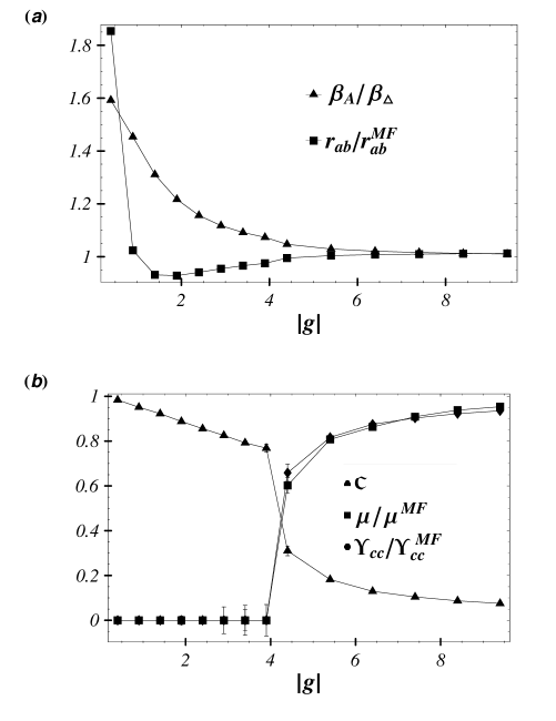
Figure 1: (a) Ratio of the mean-square gap $r_{{\mathrm{ab}}}$ [Eq. (15)] to its mean-field value $r_{\mathrm{ab}}^{MF}$, and the ratio of the generalized Abrikosov factor $\beta_{A}$ [Eq. (14)] to its value $\beta_{\Delta}$ in a triangular lattice, plotted as a function of $|g|$ [Eq. (9)]. (b) The calculated ratios of the shear modulus $\mu$ and the c-axis helicity modulus $\Upsilon_{cc}$ to their mean-field values $\mu_{MF}$ and $\Upsilon_{cc}^{MF}$, as obtained from Langevin dynamical simulations, plotted as a function of $|g|$. Also shown is ${\cal C}(T)$ [Eq. (17)]. The lattice used contains $N_{\phi}=6\times 6$ vortices in the ab-plane and $N_{z}=12$ layers in the c-direction, with periodic boundary conditions; the interlayer coupling is chosen so that $\eta|g|=0.02$. The error bars in this and later figures represent the standard deviations of results from about five Langevin dynamical simulations run for equal lengths of time.

III Results

We have solved the Langevin equations (11) numerically using a second order Runge-Kutta algorithm. In this algorithm, $\mathcal{F}$ is correct through ${\cal O}(\epsilon^{2})$ in the time step $\epsilon$. wilson In most of our simulations, we used $\epsilon=0.15\,t_{0}$; a smaller time step of $\epsilon=0.05\,t_{0}$ was found to give similar results but to require more computer time. The real and imaginary parts of the noise term $\xi_{n,k}^{\prime}(\tau)$ in Eq. (11) are chosen from Gaussian distributions with a mean zero and a variance $\sigma^{2}/\epsilon$ where $\sigma^{2}=2/[n_{x}g^{2}(B,T)]$. This choice insures that these terms have mean and variance which satisfy Eqs. (12) and (13).

In most cases, we have started our simulations from the low-temperature Abrikosov phase, then gradually increased $T$, taking the initial state for a higher $T$ as the equilibrium state for the previous slightly lower $T$. We have verified that our results exhibit only a little hysteresis - that is, we obtain the same equilibrium and nearly the same dynamical results, whether $T_{M}(B)$ is approached from below or from above. We have found that our choice of initial state generally has little effect on dynamics, providing we “anneal” our sample for a long enough time as described in the next paragraph. We have confirmed this lack of effect by obtaining similar results for various calculated dynamical quantities whether we begin by choosing an Abrikosov or a liquid-like initial state.

For each temperature considered, we have allowed the system to equilibrate for a period ranging from $10^{3}$ to $4\times 10^{6}$ time steps, before starting to compute averages, the larger number corresponding to temperatures close to $T_{M}$. We then run the dynamics for an additional $3\times 10^{4}$ to $10^{6}$ time steps at this temperature, and use these results to compute the averages.

To calculate the quantity of interest, we include in the averages only the results obtained in every $N_{0}$ time steps, where $N_{0}$ is chosen as explained below. If this procedure is used, then, according to Ref. critical, , the consecutive values included in the average become nearly statistically independent. We choose $N_{0}$ using a criterion involving the so-called self-correlator. This self-correlator is defined by the relation $C_{x}(k)=(\langle x_{i+k}x_{i}\rangle-\langle x_{i}\rangle^{2})/(\langle x_{i}^{2}\rangle-\langle x_{i}\rangle^{2})$, where $x_{i}$ is the physical quantity of interest at the $i$th time step, and $\langle...\rangle$ is a time average. With this definition, $C_{x}(0)=1$; also, $C_{x}(k)$ decreases as $k$ increases. The optimum choice of $k$ to be used in the simulations (i.e., the optimum number of steps between those included in the averages) is that which makes $C_{x}(k)$ as small as possible, typically less than $0.05$. For our simulations, we find that this optimum value of $k\equiv N_{0}$ is typically between $20$ and $50$. In general, we find that collective properties such as conductivity require much longer runs than single particle properties such as $r_{ab}$; the optimum ratio of collective to single-particle running times itself depends on the system size.

Figure 2: Normalized correlation function ${\mathcal{C}}_{J}(\tau)=\langle{\mathcal{J}}(\tau){\mathcal{J}}(0)\rangle/\langle{\mathcal{J}}(0)^{2}\rangle$ plotted as a function of $\tau$ for several values of $g$ as indicated in the Figure. The freezing transition occurs at $|g|\approx 4$ for this lattice size. Note the expanded horizontal scale. The lattice used here has $16$ vortices in each plane, and $16$ planes ($16\times 16$ lattice), and we choose $\eta|g|=0.05$.

As a test of our numerical algorithm, we have computed several equilibrium properties of the system which have been previously evaluated using Monte Carlo methods. sasik1a ; hu Our results are shown in Fig. 1. For these calculations, the lattice used contained $6\times 6$ vortices in the ab-plane and $12$ layers in the c-direction. The coupling between the layers is chosen as $\eta|g|=0.02$. We emphasize that our calculations are intended to probe a range of physically reasonable parameters, rather than to describe any specific superconductor. In Ref. hu, , $\eta|g|$ was estimated to vary from $0.0075$ (BSCCO) to $0.30$ (YBCO) in typical cuprate superconductors at temperatures and magnetic fields where the LLL approximation is likely to be valid; our choice falls well within this range.

Figure 1(a) displays the generalized Abrikosov factor $\beta_{A}/\beta_{\triangle}$ [Eq. (14)] and the quantity $r_{ab}$ [Eq. (15)] as a function of $g$ [Eq. (9)]. These results are similar to previous results obtained using the Monte Carlo method.hu In Fig. 1(b) we show the calculated $\mu/\mu^{{\mathrm{MF}}}$ [Eq. (16)] versus $|g|$. The sharp drop in $\mu/\mu^{{\mathrm{MF}}}$ near $|g|\approx 4$ is clearly visible. Although our sample sizes are quite small, the calculated equilibrium quantities still show the expected behavior of larger samples, though somewhat broadened by the substantial finite size effects.

Also shown in Fig. 1(b) is the interlayer coupling strength parameter ${\cal C}(T)$ [Eq. (17)] and the helicity modulus component $\Upsilon_{{\mathrm{cc}}}(T)$, both plotted as functions of $|g|$. Both of these quantities (which are sensitive to z-axis coherence) show a drop near $|g|\approx 4$, but ${\cal C}(T)$ is expected to vary smoothly through this region of $|g|$, while $\Upsilon_{{\mathrm{cc}}}(T)$ is expected to drop discontinuously to zero in the thermodynamic limit; some evidence of this distinction can be seen in the Figure. The simultaneous drop in $\mu/\mu^{{\mathrm{MF}}}$ and $\Upsilon_{{\mathrm{cc}}}(T)$ near $T_{M}$ suggests that there is simultaneous flux lattice melting in the ab-plane and interlayer decoupling in the c-direction, near $T=T_{M}$, consistent with previous calculations in clean systems. sasik1 ; sasik1a ; hu ; sasik2

Next, we turn to the dynamics of the system. We have calculated $\left\langle J_{z}(t/\,t_{0})J_{z}(0)\right\rangle$ as a function of various system parameters. In Fig. 2, we plot this correlation function as a function of $t/\,t_{0}$ for several values of $|g|$ both above and below the expected melting point, denoted $|g_{M}|$. ($|g_{M}|\approx 4$ for lattices of this size and our choice of parameterssasik1 ; hu ). Clearly, the decay rate slows considerably as melting is approached from higher temperatures, i.e., from smaller values of $|g|$. However, the decay rate is rapid and only weakly dependent on $|g|$ in the vortex lattice phase, $|g|>|g_{M}|$.

To make this $|g|$-dependence more apparent, we plot in Fig. 3 the half-life $\tau_{1/2}$ of this correlation function versus $|g|$ for two different system sizes, normalized by $N_{z}\,t_{0}$. $\tau_{1/2}$ is defined as the time at which $\left\langle J_{z}(t/\,t_{0})J_{z}(0)\right\rangle$ has fallen to half its $\tau=0$ value. Consistent with Fig. 2, $\tau_{1/2}$ is relatively small in both the solid and the liquid phases far from $|g_{M}|$; it increases noticeably as $|g_{M}|$ is approached from the liquid but not from the solid phase. Despite this increase, we believe that $\tau_{1/2}$ will not diverge at $|g_{M}|$, because $|g_{M}|$ corresponds to a first-order melting transition, with no dynamical critical phenomena such as a diverging correlation time.

Figures 4(a) and  4(b) show $\sigma_{c,1}(\omega^{\prime})$, as obtained from Eq. (23) for several values of $\omega^{\prime}$, and for two different system sizes. The lines simply connect the calculated points. The melting value $|g_{M}|\approx 4$, as estimated from Fig. 1(b). For $\omega^{\prime}=0.004$ and $0.008$, $\sigma_{c,1}(\omega^{\prime})$ increases strongly as $|g_{M}|$ is approached from the liquid side. There is a smaller increase at higher $\omega^{\prime}$, because the transition primarily affects fluctuations on a lower frequency scale. In the solid phase, there is little evidence of fluctuations in $\sigma_{c,1}(\omega^{\prime})$, which remains very small at nonzero frequencies for all $|g|>|g_{M}|$ studied. At fixed $|g|$ in the liquid phase near $|g_{M}|$, we expect $\sigma_{c,1}(\omega^{\prime})$ to decrease monotonically with increasing $\omega^{\prime}$; we ascribe any deviation from monotonic behavior in Fig. 4 is to numerical uncertainties. Similarly, although $\sigma_{c,1}(\omega^{\prime})$ sometimes seems to peak at a value of $|g|$ slightly smaller than $|g_{M}|$, we believe that this behavior also lies within our numerical uncertainties.

In Fig. 5 we show the total integrated fluctuation conductivity $\gamma_{2}$ [Eq. (27)], in units of $\sigma_{0}G^{2}(T)$, plotted as a function of $|g|$ for two lattice sizes. We have computed $\gamma_{2}$ using the equilibrium expression Eq. (27), which is equivalent to the frequency integral of the quantity shown in Fig. 4(a) or  4(b). As $|g_{M}|$ is approached from the liquid side; $\gamma_{2}$ falls sharply at $|g_{M}|$, to a small value in the vortex lattice phase. This drops is expected to be discontinuous in the thermodynamic (large size) limit. As previously, the full lines simply connect the calculated points. Note that $\gamma_{2}/[\sigma_{0}G^{2}(T)]$ is approximately $|g|$-independent in the liquid phase, because of the way it is normalized ($G^{2}\propto g^{2}$).

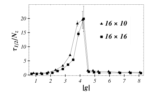
Figure 3: Half-life $\tau_{1/2}$ characterizing the decay rate of $\langle J_{z}(t/\,t_{0})J_{z}(0)\rangle$ plotted as a function of $|g|$. The full lines simply connect the calculated points. Error bars have the same meaning as in Fig. 1. The sizes of the lattice used are indicated in the Figure legend and the interlayer coupling is chosen so that $\eta|g|=0.05$.

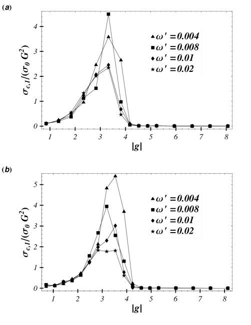
Figure 4: (a) The real part of the fluctuation conductivity, $\sigma_{c,1}(\omega^{\prime})/[\sigma_{0}G^{2}(T)]$, plotted versus $|g|$ for several values of $\omega^{\prime}$ for a $4\times 4\times 10\equiv 16\times 10$ lattice. (b) Same as (a) except that the lattice size is $4\times 4\times 16$. Note the sharp increase in $\sigma_{c,1}(\omega^{\prime})$ in the vortex liquid phase near and below $|g_{M}|$ for small $\omega^{\prime}$. The parameters are the same as in Fig. 2. For clarity, we do not show error bars; they are comparable to those of Fig. 3.

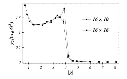
Figure 5: The integrated fluctuation conductivity $\gamma_{2}/[\sigma_{0}G^{2}(T)]$ plotted as a function of $|g|$ for two lattice sizes as shown in the Figure legend. The parameters are the same as in Fig. 2

IV Discussion

The present results are consistent with the scenario of a first-order melting transition at $T_{M}(B)$, where long-range vortex order in the ab-planes, and in the c-direction, disappear simultaneously. This interpretation is supported by the behavior of the helicity modulus $\Upsilon_{{\mathrm{cc}}}(T)$ and shear modulus $\mu(T)$, both of which vanish at the same temperature $T$. Although the present calculations are limited to relatively small samples (with fewer than $50$ vortex pancakes per plane), similar behavior has been observed in Monte Carlo simulations for considerably larger systems. sasik1 ; hu ; sasik1a

The behavior of dynamical properties, such as $\sigma_{c,1}(\omega^{\prime})$, is also consistent with first-order melting. For small $\omega^{\prime}$, $\sigma_{c,1}(\omega^{\prime})$ shows a strong increase as $T$ approaches $T_{M}$ from above. This behavior occurs because, in the solid phase, the vortex pancakes in adjacent layers lie above one another; as a result, fluctuating currents between the layers are small. On the other hand, when the lattice melts (low $|g|$ or high $T$), the vortex pancakes in adjacent layers no longer lie directly above one another; hence, fluctuating phase gradients between the layers increase the current fluctuations and the fluctuation conductivity. In the liquid phase, $\sigma_{c,1}(\omega^{\prime})$ decreases with decreasing $|g|$, because $\tau_{1/2}$ is becoming smaller. However, $\sigma_{c,1}(\omega^{\prime})$ once again appears to show a discontinuity rather than a divergence at $|g_{M}|$, consistent with the first-order nature of the transition.

Why does $\sigma_{c,1}(\omega^{\prime})$ in the liquid state, shown in Fig. 4 for several frequencies, decrease with increasing temperature $T$ above $T_{M}$? We believe this decrease occurs because, as shown in Fig. 3, $\tau_{1/2}$ decreases with increasing $T$. By contrast, the quantity $\gamma_{2}/(\sigma_{0}G^{2})$, shown in Fig. 5, behaves differently from $\sigma_{c,1}$: it has a discontinuity at $T_{M}$ but varies slowly in the liquid. The lack of any clear peak in $\gamma_{2}/(\sigma_{0}G^{2})$ near $T_{M}$ can be understood from Eq. (26), which shows that $\gamma_{2}$ is independent of $\tau_{1/2}$, depending only on equal-time current density fluctuations at $t=0$. By contrast, $\sigma_{c,1}(\omega^{\prime})$ is sensitive to $\tau_{1/2}$ especially for small $\omega^{\prime}$.

At this point, we briefly comment on a seemingly counterintuitive feature of the dynamical results shown in Figs. 4, namely, that $\sigma_{c,1}(\omega^{\prime})$ is small in the vortex lattice phase for nonzero $\omega^{\prime}$, even well below $T_{M}$. Intuitively, one might expect, since this phase is superconducting, with a finite helicity modulus in the $c$ direction, that $\sigma_{c,1}(\omega^{\prime})$ would be large in this regime. However, this behavior is actually physically reasonable; our picture of the underlying physics is the following. We believe that $\sigma_{c,1}(\omega^{\prime})$ corresponding to our model dynamics is the sum of two parts: (i) the fluctuation conductivity shown in Figs. 4(a) and  4(b) (whose integral is shown in Fig. 5; and (ii) a delta function at zero frequency, corresponding to perfect conductivity. The delta function does not appear in Fig. 4(a) or  4(b) because those calculations are carried out at finite frequency, nor does it appear in the integral shown in Fig. 5. The strength of this delta function is proportional to the helicity modulus shown in Fig. 1(b), which vanishes for $T>T_{M}$. Thus, $\sigma_{c,1}(\omega^{\prime})$ is small below $T_{M}$ simply because the fluctuation contributions to the conductivity are small in this temperature range; the system is still phase coherent in the c-direction and still has a finite helicity modulus below $T_{M}$. Although it may seem strange that $\sigma_{c,1}(\omega^{\prime})$ is small for $T<T_{M}$ and finite $\omega^{\prime}$, this behavior is not unprecedented. For example, in low-T_c s-wave superconductors, the existence of a finite gap below $T_{c}$ means that $\sigma_{1}(\omega)=0$ for $T<T_{c}$ and for $\hbar\omega$ smaller than twice the energy gap.

To our knowledge, no direct measurements of $\sigma_{c,1}(\omega^{\prime})$ have been carried out in the cuprate superconductors in the high-field, clean-limit regime where our calculations might be applicable. We therefore comment briefly on an entirely different experiment in which the reported behavior somewhat resembles that shown in Fig. 4. This is a recent study of the frequency-dependent conductivity of BiSr₂Ca₂CuO_8+δ within the ab plane at zero applied magnetic field. corson This experiment reports a rather sharp peak near $T_{c}$ in the real part of the in-plane conductivity at about 0.2 THz. This peak is thought to be due to fluctuations in the phase of the order parameter which are strongest near $T_{c}$, and weaker both above and below $T_{c}$. We believe that similar fluctuations (probably in the amplitude of the order parameter as well as the phase) are producing the increase in $\sigma_{c,1}(\omega^{\prime})$ in the present model near $T_{M}$. These fluctuations are, we believe, limited in size because the melting transition is first-order rather than continuous, and they are relatively small for $T<T_{M}$.

The present calculations may be relevant to c-axis transport at strong magnetic fields (where the LLL approximation is adequate) in a clean high-T_c superconductor (where a first-order vortex lattice melting is expected), provided a Langevin dynamics is appropriate. We have tried to estimate the numerical value of our calculated $\sigma_{c,1}(\omega^{\prime})$ [Eq. (24)] for reasonable experimental parameters. For $\omega^{\prime}\ll 1$ or $\omega t_{0}\ll 1$, $\sigma_{c,1}(\omega^{\prime})$ has the same order of magnitude as the quantity

$$\sigma_{0}\,G^{2}(T)=q^{2}\,t_{0}(2d_{0}/\pi\ell^{2}\hbar^{2})k_{B}T(\eta g)^{2}g^{2}.$$ (28)

All the quantities in this equation are easily determined except $\,t_{0}$. We attempt to estimate $\,t_{0}$ using an early paper by Schmid,schmid in which the time-dependent Ginzburg-Landau equation is derived from the original BCS theory within the Gor’kov approximation. Schmid finds that $\,t_{0}\approx h/[32\,k_{B}T_{c0}(1-T/T_{c0})(1-B/H_{c2})]$, where $T_{c0}$ is the mean-field superconducting transition temperature at $B=0$. Taking $T_{c0}\sim 80$ K, $T\sim~{}60$ K we find $\,t_{0}\sim 4~{}\times~{}10^{-14}$ sec at a field of $5$ T. Substituting this value into Eq. (28), and using $\eta g=0.05$, $g^{2}\sim 20$, and $d_{0}\sim 5$ Å, we obtain $\sigma_{0}G^{2}\sim 5\times 10^{11}$ esu, or about 0.06 $\Omega^{-1}$ cm ^-1. This conductivity is considerably smaller than the apparent c-axis conductivity in the vortex liquid state, even in a very anisotropic material such as BiSr₂Ca₂CuO_8+δ . fuchs Thus, it might be difficult to observe the fluctuation contribution in a clean anisotropic superconductor, unless we have substantially underestimated $\,t_{0}$. Such an underestimate is possible, since the calculations of Schmid are based on a microscopic theory which may not be directly applicable to the layered high-T_c materials.

Few experiments appear to have measured the c-axis resistivity at the high fields where the LLL approximation would be most accurate. Fuchs et al,fuchs working at far lower fields ($\sim 25$-$200$  Oe), have observed a simultaneous disappearance of resistivity in the ab-plane and in the c-direction (indicating a single phase transition), and an abrupt increase in the c-axis resistivity at a temperature just above that transition. However, their experiments are done at such frequencies ($\approx 72$ Hz) that the inductive contribution is very dominant in the solid phase.

Finally, we briefly discuss the fact that our calculated hysteretic effects are very small in the vicinity of the first-order melting transition. In a real experiment, one might expect some evidence of superheating or supercooling. This minimal amount of hysteresis may be due to the long annealing time before we begin to calculate thermodynamic averages. Because of this long annealing, our system can apparently attain its thermodynamic state of minimum free energy before we start computing averages.

In summary, we have studied both the equilibrium and the dynamical behavior of a layered superconductor in a strong magnetic fields by solving the time-dependent Ginzburg-Landau equations, in the lowest Landau level approximation. The effects of fluctuations are incorporated by means of a Langevin noise term. The equilibrium properties are found to exhibit behavior similar that found in previous Monte Carlo results: sasik1 ; sasik1a ; hu ; sasik2 a first-order melting transition of the vortex lattice, with a simultaneous loss of in-plane and interplane order. The dynamical properties show a strong, but not divergent, increase in the c-axis conductivity as $T_{M}$ is approached from above, with a corresponding increase, but no divergence, in the half-life $\tau_{1/2}$ of the c-axis current fluctuations.

V Acknowledgments

We gratefully acknowledge support through NSF grant DMR01-04987.

References

- (1) W. K. Kwok, J. Fendrich, S. Fleshler, U. Welp, J. Downey, and G. W. Crabtree, Phys. Rev. Lett. 72, 1092 (1994).
- (2) U. Welp, J. A. Fendrich, W. K. Kwok, G. W. Crabtree, and B. W. Veal, Phys. Rev. Lett. 76, 4809 (1996).
- (3) Ruixing Liang, D. A. Bonn, and W. N. Hardy, Phys. Rev. Lett. 76, 835 (1996).
- (4) A. Schilling, R. A. Fisher, N. E. Phillips, U. Welp, W. K. Kwok, and G. W. Crabtree, Phys. Rev. Lett. 78, 4833 (1997).
- (5) R. Šášik and D. Stroud, Phys. Rev. B 48, 9938 (1993).
- (6) R. Šašik and D. Stroud, Phys. Rev. Lett. 72, 2462 (1994).
- (7) Jun Hu and A. H. MacDonald, Phys. Rev. B 56, 2788 (1997).
- (8) H. Nordborg and G. Blatter, Phys. Rev. Lett.79, 1925 (1997); Phys. Rev. B 58, 14556 (1998).
- (9) A. K. Kienappel and M. A. Moore, Phys. Rev. B 60, 6795 (1999).
- (10) A. K. Kienappel and M. A. Moore, Phys. Rev. B 56, 8313 (1997).
- (11) Z. Tešanović and A. V. Andreev, Phys. Rev. B 49, 4064 (1994).
- (12) S. Ryu and D. Stroud, Phys. Rev. B 54, 1320 (1996).
- (13) Here we assumed that the lowest Landau level eigenstates form a complete set.
- (14) R. Šášik and D. Stroud, Phys. Rev. B 49, 16074 (1994).
- (15) B. I. Halperin and D. R. Nelson, Phys. Rev. Lett. 41, 121 (1978); D. R. Nelson and B. I. Halperin, Phys. Rev. B 19, 2457 (1979); A. P. Young, Phys. Rev. B 19, 1855 (1979).
- (16) M. E. Fisher, M. N. Barber, and D. Jasnow, Phys. Rev. A 8, 1111 (1973).
- (17) R. Kubo, M. Toda, and N. Hashitsume, Statistical Physics II: Nonequilibrium Statistical Mechanics (Springer-Verlag, New York, 1985).
- (18) See, for example, C. Ebner and D. Stroud, Phys. Rev. B 28, 5053 (1983).
- (19) G. G. Batrouni, G. R. Katz, A. S. Kronfeld, G. P. Lepage, B. Svetitsky, and K. G. Wilson, Phys. Rev. D 32, 2736 (1985).
- (20) J. J. Binney, N. J. Dowrick, A. J. Fisher, and M. E. J. Newman, The theory of critical phenomena, (Oxford University Press, New York, 1992), p. 100.
- (21) J. Corson, R. Mallozzi, J. Orenstein, J. N. Eckstein, and I. Bozovic, Nature (London) 398, 221 (1999).
- (22) A. Schmid, Phys. Kondens. Materie 5, 302 (1966).
- (23) D. T. Fuchs, R. A. Doyle, E. Zeldov, D. Majer, W. S. Seow, R. J. Drost, T. Tamegai, S. Ooi, M. Konczykowski, and P. H. Kes, Phys. Rev. B 55, R6156 (1997).