Phase diagram of the two-dimensional t-t’ Falicov-Kimball model

Abstract

The ground-state phase diagram of two-dimensional Falicov-Kimball model with nearest-neighbour and next-nearest-neighbour hoppings (characterized by $t,t^{\prime}$ constants, respectively) has been studied in perturbative regime, i.e. in the case when on-site Coulomb interaction constant $U$ is much larger than $t,t^{\prime}$ ones. The fourth-order phase diagram exhibits a rich structure, more complicated than for the ordinary Falicov-Kimball model. Possible experimental implications of the presence of nnn term are shortly discussed.

I Introduction

The Falicov-Kimball model has been proposed in 1969 to description the metal-insulator transition FK69 . Later on, it has been applied in another important problems: mixed valence phenomena Khom , crystallization and alloy formation KennLieb and others. In this model, we are dealing with two types of particles defined on a $d$-dimensional simple cubic lattice $\mathbb{Z}^{d}$: immobile “ions” and itinerant spinless “electrons”. There exist also other interpretations of the model KennLieb , FKRev .

The Hamiltonian defined on a finite subset $\Lambda$ of $\mathbb{Z}^{d}$ has the form

$$H_{\Lambda}=H_{0,\Lambda}+V_{\Lambda},$$ (1)

where

$$H_{0,\Lambda}=U\sum_{x\in\Lambda}w_{x}n_{x}-\mu_{i}\sum_{x\in\Lambda}w_{x}-\mu_{e}\sum_{x\in\Lambda}n_{x},$$ (2)

$$V_{\Lambda}=-\sum_{\langle x,y\rangle\in\Lambda}t(c^{\dagger}_{x}c_{y}+c^{\dagger}_{y}c_{x})$$ (3)

Here $c^{\dagger}_{x}$ and $c_{x}$ are creation and annihilation operators of an electron at lattice site $x\in\Lambda$, satisfying ordinary anticommutation relations. The corresponding number particle operator is $n_{x}=c^{\dagger}_{x}c_{x}$. $w_{x}$ is a classical variable taking values $0$ or $1$; it measures the number of ions at lattice site $x$. The chemical potentials of the ions and electrons are $\mu_{i}$ and $\mu_{e}$, respectively.

The Falicov-Kimball model in its basic, “backbone” form given by (2), (3) is too oversimplified to give quantitative predictions in real experiments. However, it is nontrivial lattice model of correlated electrons and captures many aspects of behaviour of such systems. It allows rigorous analysis in many situations; for a review, see FKRev . One can hope that a good understanding of this simpler model might lead to better insight into the Hubbard model, where rigorous results are rare FLU .

One can try to make the FK model more realistic by adding various terms to the “backbone” hamiltonian (2), (3) in the manner analogous to that in the original Hubbard paper Hubb . (Other possibility is enlargement of the space of internal degrees of freedom FKRev , but we will not consider it here.) The most important among them are: consideration of another types of lattice, particle statistics and presence of magnetic field GruberMMU ; correlated hopping (analysed in RefchFKM , WL1and2 , chfk3 ); taking into account the Coulomb interactions between nearest neighbours, as well as (small) hopping of heavy particles BorKot , DFF4 ; consideration of the next-nearest-neighbour hoppings (let’s name this modification as the $t-t^{\prime}$ model in analogy with the corresponding version of the Hubbard model t-t'Hub ). This last effect has been analysed in only few papers. In LeJe , authors established that if $t^{\prime}\ll t$, then the phase diagram of the $t-t^{\prime}$ FKM does not differ too much from the diagram of the pure FK model. A remarkable paper is GruKotUel , devoted to analysis of three-dimensional strongly asymmetric Hubbard model (i.e. generalized FK one) with three hopping parameters, for large Coulomb interaction constant $U$, in the neighbourhood of the symmetry point. Authors have determined rigorously the structure of ground states and proved their thermal stability up to terms proportional to $U^{-1}\times$ (square of the hopping constant).

In this paper, author examined influence of further terms of perturbation expansion (3-rd an 4-th ones) on the ground-state phase diagram in two-dimensional situation in the half-filling case, i.e. when the average value of the total particle number $\sum_{x\in\Lambda}(n_{x}+w_{x})$ is equal to the number of sites $|\Lambda|$. Effects of higher-order-terms turned out to be very interesting in the ordinary FK model GruberMMU , GUJ , Ken94 .

As a first step of the study, the effective Hamiltonian has been derived; it can be written as the Hamiltonian for the Ising model with complicated interactions, leading to strong frustration. After that, ground states of the Hamiltonian have been looked for, and the phase diagram has been constructed. In the orders 2 and 3 it was possible to determine it rigorously, whereas in the fourth order use of the restricted phase diagram method was necessary. This method proved their utility in the analysis of another versions of the FKM WL1and2 , WatsLem , FLB . In this method, one constructs collection of all periodic arrangements of ions up to certain values of lattice sites $N$ per elementary cell, and then one looks for the configuration of minimal energy among members of this set.

As one could expect, the fourth-order phase diagram turned out to be more complicated than in the case of the ordinary FKM. In this last case, one observes five phases with period not exceeding $N=5$ GruberMMU , GUJ , Ken94 ; in the case of the correlated-hopping FKM, six phases are present WL1and2 , chfk3 . In the ground state phase diagram of $t-t^{\prime}$-FKM, thirteen phases has been found (three of them are degenerate); the period of non-degenerate phases does not exceed 12 sites per elementary cell. One observes also that the region occupied by one phase (FK-like one, of density $1/4$) is anomally large (one can expect that this region should occupy region of the size of the order $t^{4}/U^{3}$, whereas the actual size is of the order $t^{\prime 2}/U$). This phenomenon can be explained by the lifting of the macroscopic degeneracy present in the second order by higher-order perturbation.

Comparing phase diagrams of the FKM and $t-t^{\prime}$ FKM, it turned out that the influence of the nnn hopping is surprisingly large.

The outline of the paper is as follows. In the Sec. II, the effective Hamiltonians up to fourth order perturbation theory have been derived. In the Sec. III, ground states and phase diagram of the effective Hamiltonians in subsequent orders have been determined. Moreover, effects of neglected higher-order-terms as well as temperature have been discussed. The last section IV contains summary and conclusions.

II Perturbation theory and effective Hamiltonian

II.1 Nonperturbed Hamiltonian, their ground states and phase diagram

In this paper we examine the model in the range of parameters $t,t^{\prime}\ll U$. The value of $t^{\prime}$ is usually smaller than that of $t$, however both these quantities are of the same order.

For derivation of the effective Hamiltonian, the method worked out in the paper DFF2 has been applied. It has this advantage that it can serve (provided certain conditions are fulfilled) as a first step to application of the quantum Pirogov-Sinai method and proving thermal and quantum stability of ground states. Detailed description of all these procedures can be found in DFF1 – DFF4 . Here, only the application of the method and results will be given, as the general scheme is identical as in the paper DFF4 .

To obtain the final expression, we must divide states of the system onto ground and excited ones, and to find corresponding projections onto both groups. These collection of states are identical as in DFF4 .

Let us begin our analysis starting from the classical part of the Hamiltonian (2); it is well known, see DFF4 . The Hilbert space ${\cal H}_{i}$ on the $i$-th site is spanned by the states: $|n_{i,+},n_{i,-}\rangle$ or, explicitely, $|0,0\rangle$, $|1,0\rangle$, $|0,1\rangle$ and $|1,1\rangle$. The corresponding energies are: $0;-\mu_{+};-\mu_{-};U-\mu_{+}-\mu_{-}$. The phase diagram consist of the following four regions. In region $I$, defined by $\mu_{+}<0,\mu_{-}<0$, all sites are empty. In two twin regions $II_{+},II_{-}$ given by conditions: $II_{+}$: $\mu_{+}>0$, $\mu_{+}>\mu_{-}$, $\mu_{-}<U$ (for $II_{-}$, one should interchange the subscripts $+$ and $-$) all sites are in the $|1,0\rangle$ (corresp. $|0,1\rangle$) state. In the region $III$, given by: $\mu_{+}>U,\mu_{-}>U$, all sites are doubly occupied. This situation is illustrated on Fig. 1.

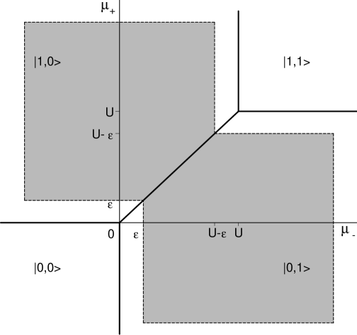
Figure 1: Phase diagram of the nonperturbed Hamiltonian (2).

We choose the states $|1,0\rangle$ and $|0,1\rangle$ as ground states. They are divided from excited ones by energy gap $\Delta={\rm min}(U,\mu_{+},\mu_{-})$. It means that we analyse the phase diagram in some subset of the region $II_{+}\cup II_{-}$ (the shaded region on the Fig. 1). The most interesting situation takes place in the neighbourhood of the $\mu_{+}=\mu_{-}$ line between regions $II_{+}$ and $II_{-}$; on this line, we observe a macroscopic degeneracy.

The projection operator on ground states at $i$-th site is

$$P^{0}_{i}=(n_{i,+}-n_{i,-})^{2}$$ (4)

II.2 Effective Hamiltonians up to 4-th order of perturbation theory

Expression for effective Hamiltonian in fourth-order perturbation theory for the ordinary FK model can be found in DFF4 , Table 2. The 4-th order effective Hamiltonian for $t-t^{\prime}$ FKM can be derived using the same methodology, described in DFF4 , Sec. 3. (It should be stressed that expressions up to 4-th order have been derived, for the 3d model, in the paper GruKotUel . Unfortunately, authors didn’t analyse effects of orders 3 and 4).

As a final result of calculations, one obtains, after specialization to the half-filled case (i.e. the situation where the total number of particles is equal to the number of lattice sites):

$\bullet\;$Second-order correction:

$$H^{(2)}_{0}=-h\sum_{i}S_{i}+\sum_{d(i,j)=1}\frac{t^{2}}{2U}(4S^{3}_{i}S^{3}_{j}-{\bf 1})+\sum_{d(i,j)=\sqrt{2}}\frac{t^{\prime 2}}{2U}(4S^{3}_{i}S^{3}_{j}-{\bf 1})$$ (5)

where: $h=\mu_{i}-\mu_{e}$; $S_{i}$ is the classical one-half spin on the lattice site $i$; it is related to the variable $w_{i}$ by the formula: $S_{i}=(w_{i}-1)/{2}$.

$\bullet\;$Third-order correction:

$$H^{(3)}_{0}=\frac{t^{2}t^{\prime}}{U^{2}}\sum_{i,j,k}\left(6\,S_{i}S_{j}S_{k}-\frac{1}{2}(S_{i}+S_{j}+S_{k})\right)$$ (6)

where summation is performed over all triples $\{i,j,k\}$ on the lattice such that $\{i,j\}$ and $\{j,k\}$ are nearest neighbour bonds forming the angle $\pi/2$.

$\bullet\;$Fourth-order correction is the most complicated one and is a sum of two-body (2b) and four-body (4b) interactions:

$$H^{(4)}_{0}=C+J^{\rm 2b}_{1}\!\!\sum_{d(i,j)=1}\!\!S^{3}_{i}S^{3}_{j}+J^{\rm 2b}_{2}\!\!\sum_{d(i,j)=\sqrt{2}}\!\!S^{3}_{i}S^{3}_{j}+J^{\rm 2b}_{3}\!\!\sum_{d(i,j)=2}\!\!S^{3}_{i}S^{3}_{j}+J^{\rm 2b}_{4}\!\!\sum_{d(i,j)=\sqrt{5}}\!\!S^{3}_{i}S^{3}_{j}+J^{\rm 2b}_{5}\!\!\sum_{d(i,j)=\sqrt{8}}\!\!S^{3}_{i}S^{3}_{j}$$

$$+J^{\rm 4b}_{1}\!\!\sum_{\pi_{1}(ijkl)}\!\!S_{i}S_{j}S_{k}S_{l}+J^{\rm 4b}_{2}\!\!\sum_{\pi_{2}(ijkl)}\!\!S_{i}S_{j}S_{k}S_{l}+J^{\rm 4b}_{3}\!\!\sum_{\pi_{3}(ijkl)}\!\!S_{i}S_{j}S_{k}S_{l}+J^{\rm 4b}_{4}\!\!\sum_{\pi_{4}(ijkl)}\!\!S_{i}S_{j}S_{k}S_{l}$$ (7)

In formulas above, we have: $C=3\tau/2+5\tau^{\prime}+3\tau^{\prime\prime}/2$; $J^{\rm 2b}_{1}=-18\tau-32\tau^{\prime}$; $J^{\rm 2b}_{2}=6\tau-36\tau^{\prime}-18\tau^{\prime\prime}$; $J^{\rm 2b}_{3}=4\tau-4\tau^{\prime}+6\tau^{\prime\prime}$; $J^{\rm 2b}_{4}=12\tau^{\prime}$; $J^{\rm 2b}_{5}=4\tau^{\prime\prime}$; $J^{\rm 4b}_{1}=40\tau+80\tau^{\prime}$; $J^{\rm 4b}_{2}=40\tau^{\prime\prime}$; $J^{\rm 4b}_{3}=40\tau^{\prime}$; $J^{\rm 4b}_{4}=40\tau^{\prime}$, where: $\tau=t^{4}/U^{3}$; $\tau^{\prime}=t^{2}t^{\prime 2}/U^{3}$; $\tau^{\prime\prime}=t^{\prime 4}/U^{3}$. Sets $\pi_{\alpha}(ijkl)$ are defined in the following way: $\pi_{1}$ (“square”) is formed by spins occupying vertices $(0,0)$, $(0,1)$, $(1,1)$ and $(1,0)$; $\pi_{2}$ (“diagonal square”) is formed by: $(0,0)$, $(1,1)$, $(0,2)$ and $(-1,1)$; $\pi_{3}$ (“big triangle”): $(0,0)$, $(0,1)$, $(0,2)$ and $(1,1)$; $\pi_{4}$: (“rhomb”) $(0,0)$, $(1,0)$, $(2,1)$ and $(1,1)$. The summation over four-body interactions in (7) is performed over all sets obtained from plaquettes $\pi_{1},\dots,\pi_{4}$ above by operations compatible with lattice symmetries (translations, rotations by multiple of $\pi/4$, reflections, inversions); the plaquette $\pi_{\alpha}(ijkl)$ occupies sites $i,j,k$ and $l$.

III Ground state phase diagrams in order 2 and 3

III.1 Order 2

The ground-state phase diagram of the system described by the Hamiltonian (5) can be obtained by rewriting the Hamiltonian in the following equivalent form:

$$H_{0}^{(2)}=\sum_{\pi_{1}(ijkl)}h^{(2)}_{0;ijkl}$$ (8)

where

$$h^{(2)}_{0;ijkl}=\frac{t^{2}}{U}(S_{i}S_{j}+S_{j}S_{k}+S_{k}S_{l}+S_{l}S_{i})+\frac{2t^{\prime\,2}}{U}(S_{i}S_{k}+S_{j}S_{l})-\frac{h}{4}(S_{i}+S_{j}+S_{k}+S_{l})$$ (9)

(lattice sites $i,j,k,l$ are arranged anticlockwise on the plaquette).

It is easy to check that the Hamiltonian rewritten in the form (9) is an m-potential (DFF1 , DFF2 , Slawny87 ; this definition is also reminded in the Appendix). In such a case, we can replace the process of minimization of energy over the whole lattice by the problem much simpler: the minimization of energy over the set of plaquette configurations. These configurations are presented on Fig. 2. It leads to the picture of the phase diagram as illustrated on Fig. 3. This diagram possess two obvious symmetries. One of them is due to symmetry of the hamiltonian (5) with respect to the change of sign $t^{\prime}\to-t^{\prime}$; the phase diagram is also symmetric with respect to such a change of sign. The second one is the symmetry of phase diagram with respect to the change $h\to-h$; however, in this case, one should also replace configurations by their mirror images (i. e. $S_{i}\to-S_{i}$).

Figure 2: Possible configurations of $2\times 2$ plaquettes. For plaquettes $ii$ and $iii$ one should take into account plaquettes obtained from those illustrated above by rotations. Small dots denote empty lattice sites (or spins “down” in the spin language), big dots – occupied lattice sites (spins “up”, respectively).

Figure 3: Ground state phase diagram in the second order perturbation theory for the Hamiltonian (8), (9). $h$ is the difference of chemical potentials. Phases $I$ and $III$ are unique (modulo rotations and translations), whereas phases $II$ are macroscopically degenerate. In order 3, the phase diagram is a small deformation of the above picture.

Phases $I_{+}$ (full) and $I_{-}$ (empty; for illustration, see configuration 0 on the Fig. 4) are build from plaquettes $i_{+}$ and $i_{-}$, respectively. These phases are unique. We have similar situation for regions $III_{\times}$ (Néel phase; Fig. 4, configuration 10) and $III_{||}$ ( Fig. 4, configuration 11 (it is an analogon of the “planar” phase in GruKotUel ). They are build from plaquettes $iii_{\times}$ and $iii_{||}$, respectively. Again, these phases are unique (modulo translations). The situation for phases $II_{+}$, $II_{-}$ differs from previous ones. These phases are build from plaquettes $ii_{+}$, $ii_{-}$, respectively (see Fig. 4, configuration No. 5 as an example); however, they are non-unique and possess macroscopic degeneration. One can easily check that there is a large dose of freedom in building of lattice configurations from these plaquettes. We encounter here situation similar to this which happens for the antiferromagnetic Ising model on triangular lattice.

III.2 Order 3

Now, let us check how the phase diagram will change under switching third-order terms on. Let us rewrite the third-order correction (6) in the equivalent “plaquette” form:

$$H_{0}^{(3)}=\sum_{\pi_{1}(ijkl)}h^{(3)}_{0;ijkl}$$ (10)

where

$$h^{(3)}_{0;ijkl}=\frac{6\,t^{2}t^{\prime}}{U^{2}}(S_{i}S_{j}S_{k}+S_{j}S_{k}S_{l}+S_{k}S_{l}S_{i}+S_{l}S_{i}S_{j})-\frac{3\,t^{2}t^{\prime}}{2U^{2}}(S_{i}+S_{j}+S_{k}+S_{l})$$ (11)

(again spins $i,j,k,l$ are arranged anticlockwise on the plaquette).

The full Hamiltonian, up to third-order terms, is the sum of terms (9) and (11). As in previous Subsection, one can check that it is an m-potential. Moreover, it turns out that the presence of third-order terms does not modify ground states of plaquettes. In the other words, plaquette configurations which were ground-states in the second order, remain ground states also in third order! This implies that degeneracy of phases $II_{+}$ i $II_{-}$ is not lifted and they still are degenerate. What does change, it is location of the boundary between phases. The difference in location of phase boundaries in orders 2 and 3 is of the order $t^{2}t^{\prime}/U^{2}$.

The phase diagram in third order possess certain kind of symmetry. It is discussed in more details in the next Subsection. At this moment, we only conclude that the phase diagram in 3. order is a small deformation of the second-order phase diagram.

III.3 Phase diagram in fourth order

Regions occupied by phases $II_{\pm}$ in both second and third order exhibit macroscopic degeneracy. One can expect that they will be sensitive against perturbations and that in some of next orders this degeneracy will be lifted. This happens yet in fourth order; we describe the situation below.

This picture has been obtained by the restricted phase diagram method. Recall that in this method, one takes into account all periodic configurations up to certain values of lattice sites $N$ per elementary cell, and then one minimizes the energy over this set of configurations.

The ground-state phase diagram is much more complicated than for the ordinary FKM – see Figs. 4 and 5 but it is still manageable (in some respects it is similar to the phase diagram of the FKM on triangular lattice, studied in GruberMMU ). Thirteen phases have been detected on phase diagram; it seems that three of them are degenerate. Moreover, for each phase present for $h>0$, there corresponds their “mirror” for $h<0$ (this mirror is obtained by the change of occupied sites onto unoccupied ones and vice versa). Periods of these phases do not exceed 12 sites per elementary cell. Such a picture emerged at $N=12$ and hasn’t changed up to $N=27$ (which corresponds to more than $3\times 10^{7}$ trial configurations). For this reason, author claims that this phase diagram is “exact but non-rigorous”.

Figure 4: Phases appearing on the ground-state phase diagram for the fourth-order effective Hamiltonian (7). Configurations: 0,2,4-11 are unique modulo lattice symmetry operations. Configurations possessing densities $1/9$, $1/6$ and $3/8$ are degenerate and form (infinite?) series; two first examples for every such a series are shown (1,1’ etc.).

Figure 5: The ground-state phase diagram for the fourth-order effective Hamiltonian (7). Only topological aspects of the phase diagram are displayed, as most of phases occupy very narrow regions. Phases: 1-4, 6-9 and 12: width of these regions is of fourth order in expansion parameter; other phases occupy regions of width of the second order in expansion parameter. Only one quarter (i.e. values $h>0,t^{\prime}>0$) are shown, as for other quarters, topological structure of the phase diagram is the same.

The phase diagram in fourth order possess certain (pseudo)symmetries. Let us describe the situation order-by-order.

In the second order, we have the Hamiltonian symmetric with respect to the change $h\to-h$ and $t^{\prime}\to-t^{\prime}$. It is obvious that the phase diagram is symmetric with respect to the change $h\to-h$, if one change also configuration to its mirror image.

In the third order, the Hamiltonian is no longer symmetric. However, their ground states are easily determined, because the Hamiltonian is expressible as a sum of m-potentials, defined on $2\times 2$ plaquettes. It turns out that on the phase diagram, there are present the same phases as in the second order. The difference between phase diagrams in the second and third order is apparent in location of phase boundaries; corresponding lines are shifted by a factor proportional to $tt^{\prime 2}/U^{2}$. This shift is symmetric with respect to the change $h\to-h$. In the other words: If some boundary between phases $i$ and $j$ is shifted by $\epsilon$ for $h>0$, then, for $h<0$, the boundary between mirrors of phases $i$ and $j$ is shifted by $-\epsilon$.

Let us analyse (pseudo)symmetries of the fourth order phase diagram. Consider first some third-order configuration of minimal energy for $h>0$ (call it CME${}^{3}_{+}$); for every such a configuration, we have its mirror, which is also the configuration of minimal energy for some $h<0$ (call it CME${}^{3}_{-}$). Now, let us add the fourth order contribution to the Hamiltonian. This term is symmetric with respect to reversing of spins; so, if for $h>0$ we have some configuration of minimal energy CME${}^{4}_{+}$, then for $h<0$ the configuration of minimal energy CME${}^{4}_{-}$ will be the mirror of CME${}^{4}_{+}$.

Let us summarize the above by the statement that the topological structure of phase diagram is the same for $h>0$ and $h<0$; for every phase $i$ appearing for $h>0$, we have corresponding mirror $\hat{i}$ for $h<0$. Phase boundaries between phases $i$ and $j$ and their mirrors $\hat{i}$ and $\hat{j}$ are related by:

$$h_{i/j}=At^{2}+A^{\prime}t^{\prime 2}+Bt^{2}t^{\prime}+Ct^{4}+C^{\prime}t^{2}t^{\prime 2}+C^{\prime\prime}t^{\prime 4}$$

$$h_{\hat{i}/\hat{j}}=-At^{2}-A^{\prime}t^{\prime 2}+Bt^{2}t^{\prime}-Ct^{4}-C^{\prime}t^{2}t^{\prime 2}-C^{\prime\prime}t^{\prime 4}$$

Let us stress that this situation (i.e. the same structure of phase diagram for $h>0$ and $h>0$ is a very peculiar property of the fourth-order Hamiltonian (5), (6), (7); it is due to degeneracy and (pseudo)symmetries of lower-order Hamiltonians. For more general Hamiltonian, we have no such similarity.

Perhaps, the most interesting effect of the presence of the term with next-nearest-neighbour hopping is the appearance of the anomally large region occupied by the phase 5 (FK-like phase with density $1/4$). At first sight, phases appearing in the fourth-order perturbation theory should occupy region of the width $p(t,t^{\prime})/U^{3}$ (where $p(t,t^{\prime})$ is some homogeneous fourth-order polynom in $t$ and $t^{\prime}$). However, it turns out that phase 5 occupies a region of width proportional to $t^{\prime 2}/U$, i.e. of the same order as the Néel phase, appearing in the second order! One can explain this phenomenon in the following way: Regions occupied by phase $II_{+}$ (the situation with phase $II_{-}$ is analogous) has width of the order $t^{\prime 2}/U$ proportional to exhibit macroscopic degeneracy both in 2-nd and in 3-rd order. The fourth-order perturbation lifts this degeneracy and as a result the phase $II_{+}$ (an ’ancestor’) transforms into non-degenerate phase 5 (the ’descendant’) of the same density, and occupies region approximately as large as an ’ancestor’ $II_{+}$.

Most of phases is unique, but there are also phases which remain degenerate even in the 4-th order (phases 1, 3, 12). Strictly speaking, the restricted phase diagram method detects here only finite degeneracy, i.e. finitely many ground states with identical energy and density but different orderings (we don’t count trivial degeneracy due to symmetry operations, i.e. translations, rotations and reflections). Number of these ground states grows with $N$; for $N=27$ we observed: eight phases of equal energy and density $1/9$, (the first two such configurations are phases 1 and 1’); eight phases of density $1/6$ (the first two such configurations are phases 3 and 3’); five phases of density $3/8$ (the first two of them are 12 and 12’). Moreover, it has been observed that every member of such collection of phases with equal density is build up from identical plaquette configurations $3\times 3$. They can be ’glued’ together in various arrangements and there is no uniqueness in such a procedure, i.e. resulting lattice configuration is non-unique. Situation here is similar to that which happens in the second order for phases $II_{\pm}$. It is natural to conjecture that we encounter here the macroscopic degeneracy, i.e. presence of infinite number of configurations of identical density and energy. However author (so far) can’t prove this.

Phase diagrams in orders 2 and 3 are rigorous (by writing out Hamiltonians as sums of m-potentials). Author tried to do analogous thing in the fourth-order by an attempt to construct m-potentials in a manner analogous as in Ken94 , GruberMMU , chfk3 , however, it succeeded only for some phases, but not for a whole phase diagram.

An analysis above concerned the ’truncated’ phase diagram, i.e. the phase diagram of the fourth-order effective Hamiltonian (7). Which changes can result as an effect coming from next (neglected) orders and temperature? Author expects (and conjectures) that most phases (i.e. all with exception of degenerate ones: i.e. 1, 3, 11 and their descendants) are stable ones DFF1 , DFF2 . For such phases, Peierls conditions (both classical and quantum ones – see DFF1 , DFF2 ) are fulfilled, and regions occupied by these phases deform in only small manner upon thermal and quantum perturbations. This assertion concerns regions of phase diagram sufficiently far from phase boundaries. For regions of width of the order of $t^{5}/U^{4}$ around phase boundaries, one cannot formulate any statements without going into next orders of perturbation theory. However, at present author cannot prove stability and Peierls conditions. (It could be proved by construction of m-potentials, which failed so far). Regions occupied by degenerate phases constitute different problem. Here, changes caused by thermal and quantum perturbations can be very significant; they are “terra incognita” and we skip this subject, leaving it as an open problem.

IV Summary and conclusions

The effective Hamiltonian and phase diagram for ground states of the $t-t^{\prime}$ FKM have been determined up to fourth order of perturbation theory. In the second and third order, phase diagram was constructed by rewritting the Hamiltonian as a sum of m-potentials. The phase diagram in the fourth order has been determined by the method of restricted phase diagrams; author claims that such a picture is “exact but non-rigorous”. The phase diagram is considerably more complicated than for the ordinary FKM, but still it is manageable. Thirteen phases are present (plus their “mirrors”); three of these phases are degenerate (i.e. possess identical density and energy but different ordering). Author conjectures that this degeneracy is macroscopic (the method of restricted phase diagrams handles only finite number of configurations).

Let us list some of the features of the phase diagram in fourth order:

1. For small $t^{\prime}$, the phase diagram is similar to this for the ordinary FKM; however, for larger $t^{\prime}$, these phase diagrams are quite different.

2. One observes anomally large region occupied by one of the phases appearing in 4-th order (phase number 5). It could have experimental implications as a possibility of appearance of “charge density waves” more exotic than Néel ordering.

3. The phase diagram of the full model (i.e. with inclusion of neglected terms perturbation theory, as well as temperature) is more difficult to examine than for the ordinary FKM. At this stage of investigation, almost nothing rigorous can be said. However, author expects that after switching the quantum and thermal perturbations on, the phase diagram will change in only small manner inside regions occupied by nondegenerate phases (0,2,4–10,12). But regions of width of the order $t^{4}/U^{3}$ around the phase boundaries, as well as regions occupied by degenerate phases 1,3,11, are out of possibilities of present analysis.

4. The Falicov-Kimball model is sensitive to perturbations. Modifications of the Hamiltonian such as introduction of correlated hopping, nnn-hopping or consideration of the FKM in non-perturbative regime (i.e. for values of $t/U$ not very small) can significantly or even drastically modify the phase diagram.

Appendix A Ground states, m-potentials

The Hamiltonian $H_{\Lambda}$ , where $\Lambda\subset\mathbb{Z}^{d}$, is a function defined on $\Omega_{|\Lambda|}$ – the space of all configurations of the system. Usually Hamiltonian is defined as a sum of potentials, i.e. functions defined on subsets of $\Lambda$: $H_{\Lambda}=\sum_{B\subset\Lambda}\Phi_{B}$. Usually one imposes restrictions such that potentials are finite-range ones, i.e. such that $|B|\leq M$, $M$ finite. It is also assumed that potentials are translation invariant.

m-potential. Now, consider the system on an infinite lattice ${\mathbb{Z}}^{d}$. Assume that sets $B_{a}$ (i.e. potential supports) are translation of a fixed plaquette $B$ by a lattice vector $a$: $B_{a}=\tau_{a}B$, where $\tau_{a}$ is an operator of such translation. We say that the function $\Phi_{B}$ is an m-potential, if there exist configuration (perhaps, non-unique) $\omega^{0}\in\Omega_{N}$ with the following properties: i) For every plaquette $B_{a}$, the “plaquette energies”, i.e. values of the Hamiltonian calculated on the plaquette $B_{a}$: $\Phi_{B_{a}}(\omega^{0})$ are all equal; ii) For every another configuration $\omega\in\Omega_{N}$, the condition: $\Phi_{B_{a}}(\omega^{0})\leq\Phi_{B_{a}}(\omega)$ is fulfilled.

Ground states of the classical Hamiltonian. If there exist such configuration $\omega^{0}\in\Omega_{N}$ as above, then we call it the ground state of the Hamiltonian.

The property of the potential to be an m-potential can be reformulated as follows. If a given potential is an m-potential, then the local minimality of energy (i.e. minimality on a plaquette) implies the global minimality on the whole lattice. The property that a potential is an m-potential is very important one, as it replaces searching of ground states of the infinite lattice by looking for the minima on a finite set. Unfortunately, some given potential possess this property only exceptionally. (But fortunately, in Secs. III.1 and III.2 they share such property!) A method to avoid this obstacle is to find – for a given potential $\Phi$ – an equivalent potential $\Phi^{\prime}$, such that $\Phi^{\prime}$ is an m-potential. However, in general it is difficult task.

Acknowledgements.

The author is grateful for numerous discussions with R. Lemański and J. Miȩkisz. This work was supported by the Polish Research Committee (KBN) under Grants: No. 2 P03B 131 19 and 110/501/SPUB/27, and by the Postdoctoral Training Program HPRN-CT-2002-00277.

References

- (1) Falicov, L. M., and Kimball, J. C.: Phys. Rev. Lett. 22, 997 (1969).
- (2) Khomskii, D. I. in Quantum Theory of Solids, Lifshitz, I. M., ed. (Mir, Moscow, 1982).
- (3) Kennedy, T. and Lieb, E. H.: Physica A 138, 320 (1986).
- (4) Gruber, C. and Macris, N.: Helv. Phys. Acta 69, 851 (1996); Gruber, C. In: Mathematical Results in Statistical Mechanics, World Scientific, Singapore, 1999; Jȩdrzejewski, J. and Lemański, R.: Acta Phys. Polon. B 32, 3243 (2001); Freericks, J. K. and Zlatić, V.: cond-mat/0301188.
- (5) Freericks, J. K., Lieb, E. H. and Ueltschi, D.: Comm. Math. Phys. 227, 243 (2002).
- (6) Hubbard, J.: Proc. Roy. Soc. London A 276, 238 (1963); A 277, 237 (1964); A 281, 401 (1964).
- (7) Gruber, Ch., Macris, N., Messager, A. and Ueltschi, D.: J. Stat. Phys. 86, 57 (1997).
- (8) Michielsen, K.: Phys. Rev. B 50, 4283 (1994); Farkasovsky, P.: cond-mat/9908094; Schiller, A.: Phys. Rev. B 60, 15660 (1999); Michielsen, K. and de Raedt, H.: Phys. Rev. B 59, 4565 (1999).
- (9) Wojtkiewicz, J. and Lemański, R.: Phys. Rev. B 64, 233103 (2001); Acta Phys. Polon. B 32, 3467 (2001).
- (10) Wojtkiewicz, J.: J. Stat. Phys. 112, 1149 (2003).
- (11) Borgs, C. and Kotecky, R.: Comm. Math. Phys. 208, 575 (2000).
- (12) Hlubina, R., Sorella, S. and Guinea, F.: Phys. Rev. Lett. 78, 1343 (1997); Avella, A., Mancini, F., Villani, D. and Matsumoto, H.: Eur. Phys. J. B 20, 303 (2001).
- (13) Lemański, R. and Jȩdrzejewski, J.: Private communication.
- (14) Gruber, Ch., Kotecky, R. and Ueltschi, D.: J. Phys. A: Math. Gen. 33, 7857 (2000).
- (15) Gruber, Ch., Ueltschi, D. and Jȩdrzejewski, J.: J. Stat. Phys. 76, 125 (1994).
- (16) Kennedy, T.: Rev. Math. Phys. 6, 901 (1994).
- (17) Watson, G. I. and Lemański, R.: J. Phys.: Condens. Matter 7, 9521 (1995).
- (18) Lemański, R., Freericks, J. K and Banach, G.: Phys. Rev. Lett. 89, 196403 (2002).
- (19) Datta, N., Fernandez, R., and Fröhlich, J.: J. Stat. Phys. 84, 455 (1996).
- (20) Datta, N., Rey-Bellet, L., Fröhlich, J. and Fernandez, R: Helv. Phys. Acta 69, 752 (1996).
- (21) Fröhlich, J. and Rey-Bellet, L: Helv. Phys. Acta 69, 821 (1996).
- (22) Datta, N., Fernandez, R. and Fröhlich, J.: J. Stat. Phys. 96, 545 (1999).
- (23) Slawny, J. In: Phase Transitions and Critical Phenomena vol. 11, C. Domb and J. Lebowitz, eds (Academic Press, London/New York 1987).