Elastic properties of a cellular dissipative structure

Abstract

Transition towards spatio-temporal chaos in one-dimensional interfacial patterns often involves two degrees of freedom: drift and out-of-phase oscillations of cells, respectively associated to parity breaking and vacillating-breathing secondary bifurcations. In this paper, the interaction between these two modes is investigated in the case of a single domain propagating along a circular array of liquid jets. As observed by Michalland and Rabaud for the printer’s instability Rabaud92 , the velocity $V_{g}$ of a constant width domain is linked to the angular frequency $\omega$ of oscillations and to the spacing between columns $\lambda_{0}$ by the relationship $V_{g}=\alpha\lambda_{0}\omega$. We show by a simple geometrical argument that $\alpha$ should be close to $1/\pi$ instead of the initial value $\alpha=1/2$ deduced from their analogy with phonons. This fact is in quantitative agreement with our data, with a slight deviation increasing with flow rate.

1 Introduction

Many studies have been devoted to the dynamics of one-dimensional patterns. One of the motivations is to seek for an equivalent of the transition to turbulence in fluids (see Bohr for a recent exhaustive report). Coullet and Iooss CoulletIooss90 have classified the possible behavior in terms of secondary instabilities linked to broken symmetries. Most of them have been observed in various experimental systems: Rayleigh-Bénard convection Dubois89 , directional solidification Flesselles91 ; Faivre92 ; Gleeson91 , Taylor-Dean flow Mutabazi93 , Taylor-Couette flow Wiener92 , directional viscous fingering between two eccentric cylinders (”printer’s instability”) Rabaud92 ; Pan93 ; Rabaud93 . These behaviors are also recovered in numerical investigations of partial differential equations governing interface instabilities ValanceMisbah94 , and also by phenomenological models coupling a base mode k and its first harmonic 2k CaroliFauve .

Our group has investigated another experimental system: a one dimensional array of liquid columns formed below an overflowing circular dish (see fig. 1-a). This system exhibits dynamical behavior Limat98 ; Brunet01 ; Limat97 similar to those observed in directional solidification or directional viscous fingering. Typical examples of spatio-temporal diagrams are displayed on figs. 2 and 3. As in ref. Limat98 ; Brunet01 , these diagrams were obtained from pictures of the dish taken from above (see insert of fig. 1-a), and by recording grey levels along a circle intersecting every column trace. Time runs from top to bottom, space (position along the dish perimeter) is plotted on the horizontal axis.

Depending on the selected conditions (flow-rate, initial columns number, possible initial imposed motions), different regimes occur, the most spectacular one being the spatio-temporal chaos in fig. 2-b. This behavior involves a complex interaction between two elementary degrees of freedom. The first degree of freedom is called a ”vascillating-breathing” mode (fig. 2-a): adjacent columns oscillate in phase-opposition, which doubles the spatial period but preserves the $(x,-x)$ symmetry. The second degree of freedom is characterized by domains of asymmetric cells that break the $(x,-x)$ symmetry. This induces a drift of the pattern Limat98 ; Brunet01 ; Limat97 .

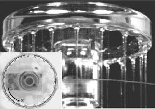
(a) (b)

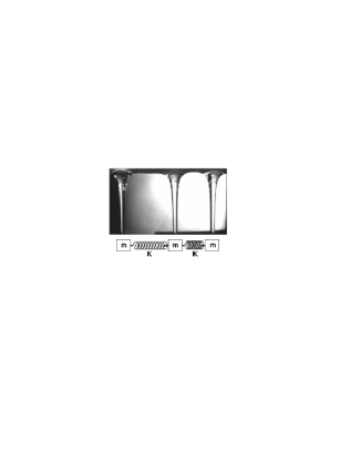
Figure 1: (a) The circular fountain experiment : a pattern of liquid columns is formed below an overflowing circular dish. Insert : viewed from above, columns appear as U-shaped spots. (b) Like in the printer’s instability Rabaud92 , it is tempting to identify the column array to a chain of springs and beads.

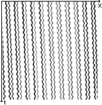
(a) (b)

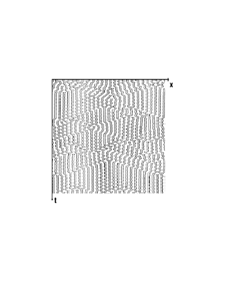
Figure 2: Spatio-temporal diagrams (I). (a) An oscillating regime (VB) extended on the whole dish ($\Gamma$ = 0.31 cm²/s, duration: $20$ s). (b) Regime of spatio-temporal chaos. Interactions between oscillations and drift sustain disorder ($\Gamma$ = 0.39 cm²/s).

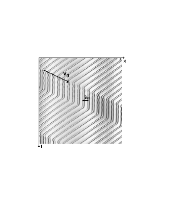
(a) (b)

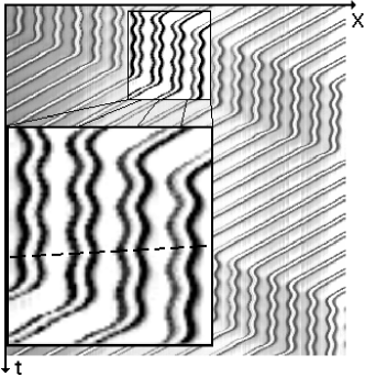
Figure 3: Spatio-temporal diagrams (II). (a) and (b) Transient oscillations following a dilation wave (PB mode) (duration = $15$ s). At low flow-rate ($\Gamma$ = 0.11 cm²/s), the VB mode is strongly damped (a). At higher flow-rate($\Gamma$ = 0.29 cm²/s), its lifetime reaches one period of rotation of the domain (b). Inserted, a magnified view. The dotted line linking the maxima of column oscillations indicates the deviation to a perfect phase opposition between neighbouring columns.

These two bifurcations have motivated several experimental Flesselles91 ; Faivre92 ; Rabaud93 ; Limat98 ; Brunet01 ; Limat97 as well as theoretical studies CoulletIooss90 ; ValanceMisbah94 ; Fauve91 ; CaroliFauve ; C3G91 ; Gil99 . Among the latter, Misbah and Valance ValanceMisbah94 noticed that for small systems, the interaction between these two modes may lead to temporal chaos. Therefore a careful examination of this interaction in our well controled system is an essential step in the study of the transition towards spatio-temporal chaos in an extended geometry. On the other hand, spatially chaotic states are so complex that informations taken from regular behavior are to be prefered at the present stage. In various systems, including our fountain experiment, the vacillating-breathing mode is known to accompany the propagation of a solitary drifting domain, which trailing edge is often followed by transient oscillations. The interaction between a solitary parity broken domain and its own oscillatory wake is thus the subject of this article.

2 Linking oscillation and drift: the phonon analogy

The idea of a possible interaction between oscillations and drift in 1D patterns is natural, but remains undiscussed at least quantitatively by available theories. For instance, models based upon the coupling between a base mode and its second harmonic (”k-2k approaches”) are able to capture both behavior analytically Fauve91 but, to our knowledge, a solution involving a wall separating oscillations and drift has never been proposed. The other well known approach based upon symmetry considerations CoulletIooss90 ; C3G91 leads to sets of coupled phase and amplitude equations that are specific to each state (oscillations and drift) and are therefore unable to handle their interaction. L. Gil Gil99 recently showed that solitary drifting domains followed by an oscillatory wake can be recovered when spatial phase shifts between a base mode and a bifurcated oscillatory mode are considered. However, this study remained only qualitative.

On the other hand, quantitative evidences of such an interaction were reported by Michalland and Rabaud for the printer’s instability Rabaud92 and confirmed by further investigations on the fountain experiment Limat98 ; Limat97 . These works all mention a relationship linking the velocity of the domain walls $V_{g}$ to the angular frequency $\omega$ of the transient oscillations left behind and the spacing $\lambda_{0}$ between columns (defined outside of the propagating domain):

$$V_{g}=\alpha\lambda_{0}\omega$$ (1)

where $\alpha$ was found in a range from 0.36 to 0.4. To interpret qualitatively this result, Michalland and Rabaud Rabaud92 suggested an analogy with the propagation of dilation waves on a lattice of springs and beads (fig. 1-b). This ”phonon approach” may seem particularly relevant in the case of liquid columns since this pattern appears as composed of discrete localized singularities Limat97 . The numerical simulation of spring and mass lattice submitted to a sudden motion of a boundary indeed reveals the propagation of dilation waves that exhibits a structure qualitatively similar to that of our drifting domains, although they are damped by dispersion on long time scales (fig. 3-a and b). The velocity of these ”domains” and the angular frequency of oscillations are linked by a relationship identical to (1), where $\lambda_{0}$ is the spacing between each mass, but with $\alpha$ = $1/2$.

Though this was not explained in details in Rabaud92 , this value of $1/2$ can be deduced from the dispersion relation of phonons $\omega=2(K/m)^{1/2}\sin|ka/2|$ governing the propagation of waves on the lattice $x_{n}=\exp i(kna-\omega t)$ (where $k$ is the wavenumber, $a=\lambda_{0}$ the lattice spacing, $K$ the spring stiffness and $m$ the mass of each ”atom”). Within this framework, the domain velocity $V_{g}$ is identified to the group velocity of phonons defined in the long wavelength limit ($k\rightarrow 0$), while the frequency of oscillations is identified at the boundary of the first Brillouin zone $(k=\pi/a)$, a limit which corresponds to spatial-period doubling.

This approach has the merit to provide a simple interpretation of (1). However it is presumably incorrect, since $\alpha$ = $1/2$ is inconsistent with the measured values (0.3 to 0.4). As recognized in Limat97 , including non-linearities and dissipation in an improved ”phonon” model does not solve this problem. This is puzzling because Michaland and Rabaud argument is rather natural and very general.

Qualitatively, we think that a different coefficient is dictated by a presumably non-linear effect: a phase-matching condition between oscillation and drift.

3 Geometrical argument

A close examination of spatio-temporal diagrams (fig. 3) shows that there is a strong tendancy for phase opposition between nearest neighbours in the transient oscillatory wake. The phonon model does not impose such a condition. We think this is the only reason for the discrepancy and postulate that columns oscillate in perfect phase-opposition with nearest neighbours in the oscillatory wake as usually assumed for a pure vascillating-breathing mode CoulletIooss90 ; ValanceMisbah94 . An idealized sketch of the column motions involved at the rear of a drifting domain is sugested on fig. 4-a . In order to obtain a stationary structure propagating uniformly with time, half a period of oscillations $\pi/\omega$ must be equal to the time it takes to the rear wall of the drifting domain to cover the spacing $\lambda_{0}$ between two oscillating columns $\lambda_{0}/V_{g}$. This geometrical argument leads to:

$$V_{g}=\frac{1}{\pi}\lambda_{0}\omega$$ (2)

and hence to $\alpha=\frac{1}{\pi}$. Our argument can also be stated as follows: since trajectories in the $(x,t)$ plane should be continuous, $V_{g}$ must be equal (in absolute value) to the phase velocity of oscillations $V_{\phi}=\omega/k$, where $k$, the wavenumber of oscillations, is equal to $\pi/\lambda_{0}$ when neighbouring cells oscillate in phase opposition. A similar idea is also perhaps underlying phase matching conditions invoked to describe defect motions in cellular patterns AlvarezdeBruyn .

4 Experimental setup

The experimental setup is simple : silicon oil (viscosity $\eta=100$ cP, surface tension $\gamma=20$ dyn/cm, density $\rho=0.97$ g/cm³ at $20^{o}C$) overflows from a horizontal circular dish (fig. 1-a) at constant flow-rate per unit length $\Gamma$. For $\Gamma$ between 0.05 cm²/s and 0.6 cm²/s, the liquid self-organizes as a pattern of liquid columns. This pattern results from a Rayleigh-Taylor instability combined with a constant liquid supply. It may bifurcate towards secondary instabilities, which lead to the phenomenology displayed on figs. 2 and 3.

As explained above, these spatio-temporal diagrams are built from pictures taken from above by a video camera, the fountain being lighten by a circular neon tube (see insert of fig. 1-a)). Columns then appear as U-shaped spots, moving along a circle of radius $R=4.8$ cm slightly smaller than that of the dish (5 cm here). The diagrams are obtained by recording grey levels along this circle. Thanks to capillary effects, the columns can be manipulated. One can adjust their number and their initial motion just by touching them with needles. The rapid coalescence of several columns with another one moving at constant speed induces a locally heterogeneous pattern, in which a ”dilation wave” followed by damped oscillations (or more rigorously a drifting parity broken domain) propagates around the dish.

As shown on 3-a and b, the length of the oscillatory wake increases with flow-rate which makes possible accurate frequency measurements. We have systematically studied such domains, varying the flow rate $\Gamma$ per unit length, and we have investigated the evolution of their wall velocity $V_{g}$, as well as that of the angular frequency $\omega$ and wavelength $\lambda_{0}$ left behind.

5 Experimental results and discussion

Figure 4: Idealized geometry involved at the rear front of a propagating parity broken domain, where the drift has to match with transient oscillations.

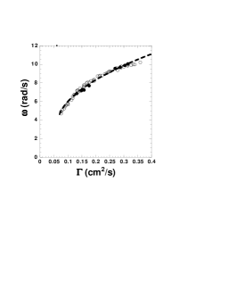
(a) (b) (c)

Figure 5: (a) Measurements of domain walls $V_{g}$ versus flow-rate. The dotted line provides a fit with power law, with an exponant of close to 0.5. (b) Angular frequency of transient oscillations left behind a drifting domain (open symbols) and in an extended oscillating state (black symbols) versus flow-rate per unit length. The fit traces a square root law with a threshold. (c) Wavelength $\lambda_{0}$ outside a propagative domain, versus flow-rate, for several domain size.

The velocity of domain walls $V_{g}$ is plotted versus flow-rate on fig. 5-a. Data are well fitted by a power law, with an exposant close to 0.5, which suggests a relationship : $V_{g}\sim\sqrt{\Gamma}$.

Measurements of the angular frequency $\omega$ of transient oscillations left behind the propagating domains are plotted on fig. 5-b versus flow-rate per unit length $\Gamma$. At a few percent of accuracy, this frequency is very close to that of global oscillations (black symbols) such as those on fig. 2-a. As in previous works Limat98 ; Brunet01 ; Limat97 , $\omega$ increases with $\Gamma$.

Figure 5-c shows measurements of the wavelength outside a propagative domain ($\lambda_{0}$). This length does not vary with flow-rate, neither with domain size. Its value is around 1.08 cm.

Despite the obvious limitations of such an approach, it is here interesting to confront this result to the ”phonon analogy”. In this point of view, assuming an effective column mass proportional to $\Gamma$, this analogy would imply that the effective stiffness $K$ could scale as $\Gamma^{2}$. This dependance is compatible with an interaction between columns through inertial terms of Navier-Stokes equation, the Reynolds number $Re=\Gamma/\nu$ being here of order 1.

In fig. 6-a, we have plotted the values of $V_{g}$ versus $\lambda_{0}\omega$. The slope appears to be very close to $1/\pi$, at low flow-rates, in agreement with eq. (2), and seems to become slightly larger when the flow-rate increases. In fact the situation is more complicated. As appears on fig. 6-b, there is a systematic difference between $V_{g}$ and $\lambda_{0}\omega$, that increases linearily with $\Gamma$, following the empirical law :

$$\frac{V_{g}}{\lambda_{0}\omega}-\frac{1}{\pi}=\frac{\Gamma-\Gamma_{c}}{D}$$ (3)

$D$ has the dimension of a diffusion coefficient. Its value is around 4.6 cm²/s. The threshold $\Gamma_{c}$ is around 0.06 cm²/s.

The effective value defined by $\alpha_{eff}=V_{g}/\lambda_{0}\omega$ varies from $0.31$ to $0.38$ linearly with flow-rate. The ”ideal” situation $\alpha=1/\pi$ implied by the argument suggested on fig. 4-a only occurs close to the limit flow-rate $\Gamma_{c}=0.06\pm 0.01$ cm²/s. It is interesting to note that this limit flow rate nearly coincides with the critical threshold of appearance of oscillations (fig. 5-b). Indeed, angular frequency measurements are correctly fitted by the following law:

$$\omega=\omega_{0}+\omega_{1}\sqrt{\frac{\Gamma-\Gamma_{c}}{D}}$$ (4)

This is consistent with a Hopf bifurcation. If this really holds, it would suggest that (1) only holds in the limit of a vanishing oscillation amplitude, the deviation from $1/\pi$ being intrinsically non-zero for any flow rate.

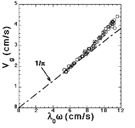
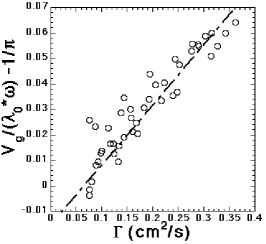
(a) (b) (c)

Figure 6: (a) Velocity of propagative domains versus the quantity $\lambda_{0}\omega$ with $\omega=2\pi/T$. (b) Difference between $V_{g}/(\lambda_{0}\omega)$ and $1/\pi$ versus flow-rate per unit length. (c) Evolution in the plane $(k,\omega)$ where $k$ is the wavenumber of the representative points of the residual oscillations. Flow rate $\Gamma$ increases from right to left, from $\Gamma$ = 0.076 cm²/s for $k$=2.83 cm^-1, to $\Gamma$ = 0.36 cm²/s for $k$=2.31 cm^-1. Black circles are based upon direct $k$ measurements from spatio-temporal diagrams, while open symbols stand for values deduced from $k=\omega/V_{g}$. The two points inside the circle correspond to negative values of $V_{g}/\lambda_{0}\omega-1/\pi$.

Finding $\alpha=1/\pi$ instead of $1/2$ shows that the liquid column array and an equivalent spring and beads sytem are rather different in the details although the analogy can perhaps be useful to get reasonable scaling laws. As we have explained, the value found for $\alpha$ seems to be dictated by : (1) a strong tendancy for neighboring columns to oscillate in perfect phase opposition and (2) a ”coherence” condition between the wall motions and the oscillations. In terms of Fourier analysis the first condition can be expressed by $k=\pi/\lambda_{0}$, i.e. the system lies at the boundary of the first Brillouin zone.

The second condition reads $V_{g}=V_{\phi}=\omega/k$, i.e. the velocity of the domain walls must be equal to the phase velocity of the oscillations. The first condition is rather reasonable if we think in terms of secondary bifurcations of a dissipative pattern. Near the threshold of oscillations, we can speculate that a single wavevector and a single frequency are selected. In some sense this mode is the sole excited eigenmode of the problem, whereas in a lattice of springs and beads, any eigenmode involved in the dispersion relation can contribute to the oscillatory wake following a dilation wave. Since $\alpha$ differs from $1/\pi$ with increasing flow-rate means that at least one of these two conditions is progressively relaxed. A careful examination of the spatio-temporal diagrams has convinced us that only the first condition is violated, the second one holding at any value of the flow rate.

This is clearly visible on the insert of fig. 3-b. Isophase lines linking second neighbours are slightly inclined, while the structure of the trajectories remains consistent with the qualitative picture of fig. 4-a. To be more quantitative, we have plotted on 6-c the path followed by the system in the plane ($k$, $\omega$) when $\Gamma$ is increased. Here we recall that $\omega$ designates the frequency of the transient oscillations, while $k$ is their wave vector (which is different from the wave vector of the pattern $k_{0}$), so that locally the column position varies as $\exp[i(kx-\omega t)]$. The black symbols are obtained by direct determinations of $k$ on spatio-temporal diagrams across slope measurements of the isophase line linking second neighbors (dotted line on fig. 3-a). This slope $\psi$ reads:

$$\tan\psi=\frac{1}{\omega}(k-\pi/a)$$ (5)

The open symbols are obtained by using the relationship $k=\omega/V_{\phi}$, and assuming $V_{\phi}=V_{g}$. The fact that both kind of symbols overlap shows that for any value of $\Gamma$, the relationship $V_{\phi}=V_{g}$ holds. Since the flowrate $\Gamma$ increases from right to left of this graph, the wave number $k$ of perturbations of columns positions is equal to $\frac{\pi}{\lambda_{0}}$ = 2.9 cm^-1 at low flow rate and progressively decreases when $\Gamma$ increases. In other words, the system initialy lies at the boundary of the Brillouin zone, and as $\Gamma$ increases, $k$ becomes smaller than $\pi/\lambda_{0}$, the perfect phase opposition is progressively lost.

6 Conclusions - Conjectures

In summary, this paper reports accurate measurements which allow us to evidence a fundamental relationship linking the velocity of a propagating parity broken domain to the frequency of its oscillatory wake. At a few percent of accuracy , this pulsation coincides with that of the oscillatory mode itself observed alone in an extended geometry (fig. 5-b), which suggests that it is finaly this oscillatory mode that rules the propagation of parity broken domain. Similarities and differences with phonons on a lattice of springs and beads have been discussed in the plane $(k,\omega)$, the residual oscillations exhibiting a possible shift of the wavenumber $k$ with respect to the boundary of Brillouin zone of order of 20 $\%$ of the maximal $k$ value.

We believe that the problem adressed in this article is important for several reasons. First, models based upon symmetry arguments CoulletIooss90 miss the relationship reproduced in eq. (2). In this approach, $\omega$ is just a free parameter that is selected at will to rebuild the spatio-temporal diagrams starting from the amplitude evolutions. This suggests that improvements of this approach must be built Gil99 . In another direction, it is to note that k-2k models Fauve91 ; CaroliFauve are able to capture both oscillations and drift. Therefore, a possible promising other idea to interpret our result would consist in building a model of the wall separating oscillations and drift by starting from Caroli et al equations suggested in ref.CaroliFauve . This could constitute a better framework to recover eq.1 by a rigorous calculation.

Next, the point investigated here has something to do with an insufficiently studied problem, i.e. that of Galilean invariance in pattern dynamics. For instance, Coullet and Fauve CoulletFauve85 studied the effect of this invariance on a Ginzburg-Landau-like equation and discussed the consequences for systems in which this invariance is slightly broken by rigid boundary conditions. Another paper from Shraiman Shraiman86 is also available in the case of the Kuramoto-Shivashinsky equation. Both papers show that, in such systems, a phase dynamics of second order in time should be observed. This second order time dynamics is an alternative to the idea to invoke a column or cell inertia. Finaly, this subtle interaction between oscillations and drift is certainly important in the genesis of spatio-temporal chaos, because it can influence the nucleation process of defects, via ”shock” formations in the phase field. We hope that our paper will motivate further studies in this field.

References

- (1) S. Michalland M. Rabaud, Physica D 61(1991) 197.
- (2) T. Bohr, M.H. Jensen, G. Paladin A. Vulpiani, Dynamical systems approach to turbulence (Cambridge University Press, 1998).
- (3) P. Coullet G. Iooss, Phys. Rev. Lett. 64 (1990) 866.
- (4) F. Daviaud, M. Dubois P. Bergé, Europhys. Lett. 9 (1989) 441.
- (5) J.-M. Flesselles, A.J. Simon A.J. Libchaber, Adv. Phys. 40 (1991) 1.
- (6) G. Faivre J. Mergy, Phys. Rev. A 45 (1992) 7320.
- (7) J.T. Gleeson, P.L. Finn P.E. Cladis Phys. Rev. Lett. 66 (1991) 236.
- (8) I. Mutabazi C.D. Andereck Phys. Rev. Lett. 70 (1993) 1429.
- (9) R. Wiener D.F. MacAlister Phys. Rev. Lett. 69 (1992) 2915.
- (10) L. Pan J.R. de Bruyn Phys. Rev. Lett. 70 (1993) 1791.
- (11) H.Z. Cummins, L. Fourtune M. Rabaud, Phys. Rev. E 47 (1993) 1727.
- (12) C. Misbah A. Valance Phys. Rev. E 49 (1994) 166.
- (13) C. Counillon, L. Daudet, T. Podgorski L. Limat, Phys. Rev. Lett. 80 (1998) 2117.
- (14) P. Brunet, J.-M. Flesselles L. Limat, Europhys. Lett. 56 (2001) 221.
- (15) F. Giorgiutti L. Limat, Physica D 103 (1997) 590.
- (16) S.Fauve, S. Douady O. Thual, J. Phys. (Paris) 1 (1991) 311.
- (17) B. Caroli, C. Caroli S. Fauve, J. Phys. (Paris) 2 (1992) 281.
- (18) R.E. Goldstein, G.H. Gunaratne, L. Gil P. Coullet, Phys. Rev. A 43 (1991) 6700.
- (19) L. Gil, Europhys. Lett. 48 (1999) 156.
- (20) R. Alvarez, M. van Hecke and W. van Saarloos, Phys. Rev. E, 56 (1997) R1306. See also P. Habdas, M.J. Case and J.R. de Bruyn, Phys. Rev. E 63 (2001) 066305
- (21) B.I. Shraiman, Phys. Rev. Lett. 57 (1986) 325.
- (22) P. Coullet S. Fauve, Phys. Rev. Lett. 55 (1985) 2857.