Rashba coupling in quantum dots: exact solution

Abstract

We present an analytic solution to the problem of the Rashba spin-orbit coupling in semiconductor quantum dots. We calculate the exact energy spectrum, wave-functions, and spin–flip relaxation times. We discuss various effects inaccessible via perturbation theory. In particular, we find that the effective gyromagnetic ratio is strongly suppressed by the spin-orbit coupling. The spin-flip relaxation rate has a maximum as a function of the spin-orbit coupling and is therefore suppressed in both the weak- and strong coupling limits.

In recent years, spin-orbit (SO) effects in quantum dots attracted much attention, as it has become clear that these effects play a crucial role in the novel field of spintronics spintronics .

The combination of a confined geometry and SO coupling has interesting consequences for the electron spectrum spectrum . Since future quantum computation devices would have to control coherent spin states over sufficiently long time–scales loss1 , it is important to understand spin relaxation mechanisms, most of which are rooted in the SO coupling.

SO interactions can arise in quantum dots by various mechanisms related to electron confinement and symmetry breaking and are generally known as the Rashba term rashba and the Dresselhaus term dresselhaus . For most experimental realisations, quantum dots can be described as effectively two–dimensional systems in a confining potential which is usually modelled as hard-wall or harmonic confinement.

To our knowledge all existing theoretical studies of SO effects in such systems rely on perturbative schemes or numerical simulations. The purpose of this paper is to provide an exact solution of the quantum mechanical problem of the combined effects of the SO coupling, confinement, and magnetic field.

In the bulk (i.e. without confinement), the problem was solved in the original paper rashba , see also br , while the effects of the confining potential (but without SO coupling) were studied in Ref.belgians . We shall show here how these exact solutions can be combined and generalised.

The one-particle Hamiltonian describing an electron in a two-dimensional quantum dot is of the form:

$$H=\frac{{\bf p}^{2}}{2m}+V(\rho)+\alpha_{R}(p_{x}\sigma_{y}-p_{y}\sigma_{x})+\frac{1}{2}g\mu_{B}B\sigma_{z}\;,$$ (1)

where $m$ is the effective electron mass, $g$ is the effective gyromagnetic ratio, and $\mu_{B}$ is the Bohr magneton. A constant magnetic field $B$ is introduced via the Zeeman term above and the Peierls substitution, ${\bf p}=-i{\bf\nabla}-\frac{e}{c}{\bf A}$ (we use the axial gauge, $A_{\rho}=0$ and $A_{\varphi}=B\rho/2$); $\alpha_{R}$ is the strength of the SO coupling, the Pauli matrices are defined as standard, the electron charge is $e=-|e|$, and we set $\hbar=1$. In (1), $V(\rho)$ is the (symmetric) confining potential. In this paper we will consider a hard-wall confining potential, i.e. $V(\rho)=0$ for $\rho<R$ and $V(\rho)=\infty$ for $\rho>R$, $R$ being the radius of the dot. We have included the Rashba term rather than the Dresselhaus term, which would be of the form $\alpha_{D}(p_{x}\sigma_{x}-p_{y}\sigma_{y})$. (The Rashba term maybe dominant, since the coupling strength $\alpha_{R}$ can be varied by system design, e.g., values of $\alpha_{R}\simeq 6\times 10^{-9}$eV cm were reported for InAlAs/InGaAs structures cui , whereas the typical values of $\alpha_{D}$ are about $10^{-9}$eV cm nazarov .) These terms transform into each other under the spin rotation: $\sigma_{x}\leftrightarrow\sigma_{y}$, $\sigma_{z}\leftrightarrow-\sigma_{z}$. So our results will only need a trivial modification in the case when a solo Dresselhaus term is present.

Hamiltonian (1) commutes with the $z$–projection of the total momentum operator $j_{z}=l_{z}+\frac{1}{2}\sigma_{z};$ $l_{z}=-i\partial_{\varphi}$ (assuming the axial gauge). The operator $j_{z}$ is therefore conserved. The eigenfunctions of the total momentum operator, with a half–integer eigenvalue $j$, are of the form:

$$\psi_{j}(\rho,\varphi)=(e^{i(j-1/2)\varphi}f_{j}(\rho),e^{i(j+1/2)\varphi}g_{j}(\rho)).$$ (2)

In zero field there is an additional symmetry $j_{z}\to-j_{z}$ related to time inversion. The states with the projections of momenta equal to $j$ and $-j$ are Kramers doublets. Introducing the operators, $\nabla^{(B)}_{\pm,j}=\pm\frac{d}{d\rho}-\frac{j}{\rho}-\frac{eB}{c}\rho\;,$ and

$$\Delta^{(B)}_{j}=\frac{1}{\rho}\frac{d}{d\rho}\left(\rho\frac{d}{d\rho}\right)-\frac{1}{\rho^{2}}\left(j-\frac{eB}{2c}\rho\right)^{2}\;,$$

the Schrödinger equation becomes,

$$\begin{array}[]{c}\Delta^{(B)}_{j-1/2}f_{j}+2m\left[E-\frac{1}{2}g\mu_{B}B-V(\rho)\right]f_{j}-2m\alpha_{R}\nabla_{-,j+1/2}^{B}\,g_{j}=0\;,\\ \Delta^{(B)}_{j+1/2}g_{j}+2m\left[E+\frac{1}{2}g\mu_{B}B-V(\rho)\right]g_{j}-2m\alpha_{R}\nabla_{+,j-1/2}^{B}\,f_{j}=0\;.\end{array}$$ (3)

We first assume that the magnetic length $a_{B}=\sqrt{c/|e|B}$ is large compared to $R$, so that the orbital effects of the magnetic field can be neglected. Working with the dimensionless coordinate $x=\rho/R$, the system of equations (3) becomes

$$\begin{array}[]{c}(\Delta^{(0)}_{j-1/2}+\epsilon-h)f_{j}-\beta_{R}\nabla^{(0)}_{-,j+1/2}g_{j}=0\;,\\ (\Delta^{(0)}_{j+1/2}+\epsilon+h)g_{j}-\beta_{R}\nabla^{(0)}_{+,j-1/2}f_{j}=0\;,\end{array}$$ (4)

supplemented by the boundary conditions $f_{j}(1)=g_{j}(1)=0$. We have introduced two dimensionless parameters, $\beta_{R}=2\alpha_{R}mR$ and $h=mg\mu_{B}R^{2}B$, characterising the strength of the SO coupling and the Zeeman term, respectively. The energy parameter is $\epsilon=2mER^{2}$.

In the absence of the Rashba term and confinement potential, the solutions regular at the origin are $f_{j}(x)\sim J_{j-1/2}(kx)$ and $g_{j}(x)\sim J_{j+1/2}(kx)$ with $k^{2}=\epsilon\pm h$, where $J_{l}(x)$ are the Bessel functions. Due to the standard recurrence relations

$$\left(\frac{d}{dx}+\frac{j\pm 1/2}{x}\right)J_{j\pm 1/2}(kx)=kJ_{j\mp 1/2}(kx)\;,$$ (5)

the Rashba term simply acts as rising or lowering operator on the Bessel functions basis rashba . Therefore the following ansatz

$$(f_{j}(x),g_{j}(x))=(d_{1}J_{j-1/2}(kx),d_{2}J_{j+1/2}(kx))$$ (6)

solves the bulk problem in the presence of the SO coupling, provided that the coefficients $d_{1,2}$ satisfy the eigenvalue equation:

$$\left[\begin{array}[]{cc}k^{2}-\epsilon+h&-\beta_{R}k\\ -\beta_{R}k&k^{2}-\epsilon-h\end{array}\right]\left[\begin{array}[]{c}d_{1}\\ d_{2}\end{array}\right]\;=0.$$ (7)

When considering the electron confined to the disk, it is seemingly impossible to impose the vanishing boundary conditions on the ansatz (6) as Bessel functions with different indices are involved. Note, however, that as long as either $\beta_{R}$ or $h$ is non–zero, the bulk spectrum has two branches: $\epsilon=k^{2}\pm\sqrt{\beta_{R}^{2}k^{2}+h^{2}}\;.$ Therefore for a given value of $\epsilon$ there are, in fact, two non-trivial solutions for the momentum $k$,

$$k_{\pm}^{2}=\frac{(2\epsilon+\beta_{R}^{2})\pm\sqrt{\beta_{R}^{4}+4\epsilon\beta_{R}^{2}+4h^{2}}}{2}\;.$$

We choose the amplitude ratios as $d_{1}^{+}/d_{2}^{+}=\alpha_{+}$ and $d_{2}^{-}/d_{1}^{-}=\alpha_{-}$, where $\alpha_{\pm}(\epsilon,\beta_{R},h)=\beta_{R}k_{\pm}/(k^{2}_{\pm}-\epsilon\pm h)\;.$ We are now able to satisfy the boundary conditions by combining these two linearly independent degenerate solutions:

$$(f_{j}(x),g_{j}(x))=d^{+}(\alpha_{+}J_{j-1/2}(k_{+}x),J_{j+1/2}(k_{+}x))$$

$$+d^{-}(J_{j-1/2}(k_{-}x),\alpha_{-}J_{j+1/2}(k_{-}x))\;.$$ (8)

The boundary conditions lead to the eigenvalue equation

$$FJ_{j+1/2}(k_{+})J_{j-1/2}(k_{-})+J_{j+1/2}(k_{-})J_{j-1/2}(k_{+})=0\;,$$

where the function $F=-\beta_{R}^{2}k_{+}k_{-}/((k_{+}^{2}-\epsilon+h)(k_{-}^{2}-\epsilon-h))\;.$ Notice that in the energy region $|\epsilon|<h$, $k_{-}$ becomes purely imaginary $k_{-}\to i\kappa_{-}$, and the respective Bessel function becomes a modified one, $I(\kappa_{-}x)$.

In the absence of the Zeeman term we have $k_{\pm}=\sqrt{\epsilon+\beta_{R}^{2}/4}\pm\beta_{R}/2$ and $d_{1}^{\pm}=\pm d_{2}^{\pm}$ , so that $F=1$ in the above equation. In this case, the equation is invariant under the change $j\rightarrow-j$ (Kramers degeneracy). At $\beta_{R}=0$ all states with $l\neq 0$ are four-fold degenerate, while $l=0$ states are doubly degenerate. According to the standard analysis, the SO coupling splits all the $l\neq 0$ states into two Kramers doublets with $j=l+1/2$ and $j=l-1/2$, while $l=0$ states naturally remain Kramers doublets. The specifics of the Rashba term is that, at small $\beta_{R}$, the SO splitting starts at the order $\beta_{R}^{2}$. The evolution of the first few energy levels with the parameter $\beta_{R}$ is shown in Fig. 1. (Values of $m\approx 0.05m_{e}$ and $g\approx-0.4$, typical for $\rm A_{3}B_{5}$ structures, are used.) We label the energy eigenstates as $(j,n)$ where $n$ is a non-negative integer such that $E_{j,n}<E_{j,n+1}$ at $\beta_{R}=0$.

Figure 1: Rashba splittings. Energy as a function of $\beta_{R}$ for the states $(1/2,0)$ (a), $(3/2,0)$ (b), $(1/2,1)$ (c), $(5/2,0)$ (d), $(3/2,1)$ (e), and $(1/2,2)$ (f). ($R=10nm$, $B=0$.)

A comparison of the exact splittings to the perturbative ones is shown in Fig. 2. As one can see from this figure, the perturbation theory seriously (by 20-30%) overestimates Rashba splittings for realistic values of the parameter $\beta_{R}$.

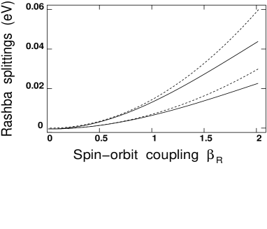
Figure 2: Rashba splittings. Energy differences $E(1/2,1)-E(3/2,0)$ and $E(3/2,1)-E(5/2,0)$ as a function of $\beta_{R}$. Dashed lines correspond to the same quantities calculated at the second-order of perturbation theory. ($R=10nm$, $B=0$.)

Upon inclusion of the Zeeman term, all Kramers doublets are also split so that all the degeneracy is completely lifted. Because of inherently small values of the gyromagnetic ratio $g$ in the semiconductor quantum dots, for realistic magnetic fields the Zeeman splittings are small ($10^{-1}$–$10^{-2}$ meV ) in comparison to the characteristic energy separation between the levels. Because of the same reason, all the Zeeman splittings can be regarded as linear in the magnetic field. So, for the Zeeman splitting of the $j$’s eigenstate we may write $\delta\epsilon_{j}=2hf_{j}(\beta_{R})\;,$ where the function $f_{j}(\beta_{R})$ [$f(0)=1$] plays the role of an effective gyromagnetic ratio, which non-trivially depends on $\beta_{R}$. Indeed, expanding the eigenvalue equation in $h$, we find the following analytic formula for the gyromagnetic factor:

$$f_{j}(\beta_{R})=t\left[\frac{J^{\prime}_{j-1/2}(k_{+})}{J_{j-1/2}(k_{+})}-\frac{J^{\prime}_{j+1/2}(k_{+})}{J_{j+1/2}(k_{+})}-(k_{+}\leftrightarrow k_{-})\right]^{-1},$$

where the prefactor is $t=4(\epsilon+\beta_{R}^{2}/4)/(\beta_{R}\epsilon)$; $\epsilon$ and $k_{\pm}$ are zero–field solutions. Numerical calculations show that $f(\beta_{R})$ is suppressed by about 50% when $\beta_{R}$ reaches 1.5. Increasing $\beta_{R}$ suppresses the Zeeman splitting because the SO coupling entangles the spin degree of freedom, making it more difficult to polarise.

The SO coupling is the main intrinsic mechanism for electron spin-flip transitions in quantum dots nazarov . In previous calculations of the spin–flip rates, the SO coupling was considered as a perturbation, so that the electron spin and angular momentum were assumed to be independently conserved. In the full theory this is not the case. The ‘spin-flip’ transitions in fact occur between the states $j$ and $-j$. No such transition is possible within a degenerate Kramers doublet (Van Vleck cancellation). In the external magnetic field, the states $j$ and $-j$ are split by the Zeeman interaction. The SO coupling allows then for phonon assisted transitions between the Zeeman sublevels (of a given Kramers doublet). We concentrate on the most interesting case and consider the spin–flip transition rate between the Zeeman sublevels of the ground state ($j=\pm 1/2$). Acoustic phonons dominate these processes at low temperatures. We consider piezoelectric interaction between the electrons and the acoustic phonons. The rate for the one–phonon transition within Zeeman sublevels is given by the Fermi golden rule. In analogy Ref.nazarov , we obtain (at zero temperature):

$$W=\frac{\Bigl{(}e\;h_{14}\;R\Bigr{)}^{2}\;(\Delta E_{Z})^{3}}{\rho_{0}s^{5}}\;F^{2}\;K,$$

$$F=\int_{0}^{2\pi}\;\int_{0}^{1}\;\cos\phi\;\psi_{-1/2}^{*}(x,\phi)\;\psi_{1/2}(x,\phi)x^{2}dx\;d\phi$$ (9)

where $s^{-5}=3/2s_{l}^{5}+1/s_{t}^{5}$, $K=8/105\pi$, $\Delta E_{Z}$ is the energy difference between the states involved, $h_{14}$ is the non-zero component of the piezo-tensor and $\rho_{0}$ is the mass density. The exact evolution of the spin–flip transition rate with the parameter $\beta_{R}$ for fixed $h$ is shown in Fig. 3. We use typical material parameters for GaAs-type structures rem . An interesting feature of the exact solution is the emergence of a maximum in the transition rate as a function of the spin-orbit coupling. The physical explanation is that while the Zeeman energy splitting decreases with $\beta_{R}$, the electron-phonon matrix element saturates. For small $\beta_{R}$ and $h$, we obtain $F\sim\beta_{R}h$ so that the transition rate is $W\sim h^{5}\beta_{R}^{2}$, in accordance with the perturbative result of Ref.nazarov .

Figure 3: The ground-state spin-flip relaxation rate $W$ as a function of $\beta_{R}$ for $B=1.5$T and $R=10$ nm.

So far we have assumed that $a_{B}>R$, which is the case for most experimental set-ups. For bigger dots and stronger magnetic fields, however, the orbital effects of the magnetic field can not be neglected. Fortunately, because of the very nature of the Peierls substitution, which has to be performed both in the kinetic energy term and in the SO term, the above analytic solution can be generalised to this case.

Using the dimensionless variable $\xi=\rho^{2}/(2a_{B}^{2})$ we propose the ansatz

$$(f_{j}(\xi),g_{j}(\xi))=(d_{1}\Phi(e_{0},j,\xi),d_{2}\Phi(e_{0}+1,j+1,\xi))\;,$$

where

$$\Phi(e_{0},j,\xi) = c_{j}\xi^{\frac{|l|}{2}}M(-e_{0}+\frac{l+|l|}{2},|l|+1,\xi)$$

$$c_{j} = \left(\frac{\Gamma(e_{0}-\frac{l-|l|}{2}+1)}{\Gamma(e_{0}-\frac{l+|l|}{2}+1)}\right)^{\frac{1}{2}}\frac{(-1)^{\frac{-l+|l|}{2}}}{\Gamma(|l|+1)}$$

with $l=j-\frac{1}{2}$ and $M(a,c;\xi)$ is the confluent hypergeometric function (see bateman ).

Figure 4: The spectrum in the orbital field. Energy as a function of magnetic field for the states $(1/2,0)$ (a1), $(3/2,0)$ (b1), $(1/2,1)$ (c1), $(5/2,0)$ (d1), $(3/2,1)$ (e1), and $(1/2,2)$ (f1), $(-1/2,0)$ (a2), $(-3/2,0)$ (b2), $(-1/2,1)$ (c2), $(-5/2,0)$ (d2), $(-3/2,1)$ (e2) and $(-1/2,2)$ (f2). ($R=50nm$, $\beta_{R}=3.35$.)

The factors $c_{j}$ are inspired by the normalisation in the standard Landau problem and $e_{0}$ is the ‘energy’ parameter to be determined. As before, we find two non-trivial solutions for it:

$$e_{0}^{\pm}=\frac{2e-1+\gamma^{2}\pm\sqrt{(\gamma^{2}+1)^{2}+4e\gamma^{2}+4(s^{2}-s)}}{2}\;.$$

We have introduced dimensionless parameters: $e=E/\omega_{c}-1/2$ ($\omega_{c}=|e|B/mc$) for the energy (not to be confused with the electron charge), $\gamma=\alpha_{d}(2m/\omega_{c})^{1/2}$ for the SO coupling, and $s=gm/(4m_{e})$ for the Zeeman coupling. Here $m_{e}$ is the electron mass. The boundary conditions then lead to the eigenvalue equation:

$$\frac{\Phi(e_{0}^{+},l,\xi_{0})\Phi(e_{0}^{-}+1,l+1,\xi_{0})}{\Phi(e_{0}^{-},l,\xi_{0})\Phi(e_{0}^{+}+1,l+1,\xi_{0})}=\frac{(e_{0}^{-}+1)^{\frac{1}{2}}}{(e_{0}^{+}+1)^{\frac{1}{2}}}\frac{e_{0}^{+}-e+s}{e_{0}^{-}-e+s},$$

where $\xi_{0}=R^{2}/(2a_{R}^{2})$. This equation provides all the information about the energy spectrum of the system. We have investigated it numerically. The results are shown in Fig. 4. Note that the Zeeman splittings are still small for realistic fields. The Kramers doublets therefore survive the orbital field as long as there is no SO coupling. It is the combined effect of the orbital field and the Rashba term that lifts the Kramers degeneracy.

To conclude, we presented an analytic solution to the problem of an electron in a quantum dot in the presence of both the magnetic field and SO coupling. We calculated various quantities of physical interest. For realistic parameters, the Rashba energy splittings are overestimated in perturbation theory. There is also a strong suppression of the effective gyromagnetic ratio by the SO coupling. The spin-flip relaxation rate has a maximum as a function of the SO coupling, a prediction that would be interesting to verify experimentally. Inclusion of the orbital magnetic field gives rise to a rich magneto-optical spectrum. We hope that our solution can be used in future research for obtaining further interesting results on the SO effects in quantum dots.

We are grateful to Levitov, who has independently arrived at a similar solution with Rashba levitov , for interesting discussions. G.L.’s and A.O.G.’s research is supported by the EPSRC grants GR/N19359 and GR/R70309 and the EU training network DIENOW. E.T.’s research is supported by the Centre for Functional Nanostructures of the Deutsche Forschungsgemeinschaft within project A2.

Note added After completion of this work we learnt that the particular case of zero magnetic field was analised by Bulgakov and Sadreev sad .

References

- (1) S.A. Wolf it et al, Science 294, 1488 (2001).
- (2) M. Governale, Phys. Rev. Lett. 89, 206802 (2002), see also C.F. Destefani, S.E. Ulloa, and G.E. Marques, cond-mat/0307027 and references therein.
- (3) D. Loss and D.P. DiVincenzo, Phys. Rev. A 57, 120 (1998).
- (4) E.I. Rashba, Fiz. Tverdogo Tela 2, 1224 (1960) [Sov. Phys. Solid State 2, 1109 (1960)].
- (5) G. Dresselhaus, Phys. Rev. 100, 580 (1955).
- (6) Yu.A. Byckov and E.I. Rashba, Pis’ma Zh. Eksp. Teor. Fiz. 39, 66 (1984) [JETP Lett. 39, 78 (1984)]; J. Phys. C 17, 6039 (1984).
- (7) F. Geerinckx, F.M. Peeters, and J.T. Devreese, J. Appl. Phys. 68(7), 3435 (1990).
- (8) L.J. Cui, Y.P. Zeng, B.Q. Wang, Z.P. Zhu, L.Y. Lin, C.P.Jiang, S.L. Guo, and J.H. Chu, Appl. Phys. Lett. 80, 3132 (2002).
- (9) A.V. Khaetskii and Yu. V. Nazarov, Phys. Rev B 61, 12 639 (2000); ibid. 64, 12 516 (2001).
- (10) Typical material parameters are: eV/cm, cm/sec, g/cm3.
- (11) Bateman Manuscript Project, Higher Transcendental Functions, Vol. I, New York (1953).
- (12) L. Levitov and E.I. Rashba (unpublished notes).
- (13) E.N. Bulgakov and A.F. Sadreev, JETP Letters, 73, 505, (2001).