Geometric effects on $T$-breaking in $p+ip$ and $d+id$ superconductors

Abstract

Superconducting order parameters that change phase around the Fermi surface modify Josephson tunneling behavior, as in the phase-sensitive measurements that confirmed $d$ order in the cuprates. This paper studies Josephson coupling when the individual grains break time-reversal symmetry; the specific cases considered are $p\pm ip$ and $d\pm id$, which may appear in Sr₂RuO₄ and Na_xCoO${}_{2}\cdot$(H₂O)_y respectively. $T$-breaking order parameters lead to frustrating phases when not all grains have the same sign of time-reversal symmetry breaking, and the effects of these frustrating phases depend sensitively on geometry for 2D arrays of coupled grains. These systems can show perfect superconducting order with or without macroscopic $T$-breaking. The honeycomb lattice of superconducting grains has a superconducting phase with no spontaneous breaking of $T$ but instead power-law correlations. The superconducting transition in this case is driven by binding of fractional vortices, and the zero-temperature criticality realizes a generalization of Baxter’s three-color model.

I Introduction

Several materials are now believed to support superconducting states where the order parameter $\Delta({\bf k})$ is complex-valued and hence breaks time-reversal symmetry. This class includes the recently reported superconductorTakada et al. (2003) Na_xCoO${}_{2}\cdot$(H₂O)_y, which is a doped Mott insulator since CoO₂ is a layered triangular-lattice spin-half antiferromagnet. RVB-type mean-field theoriesBaskaran (2003)^,Wang et al. ; Kumar and Shastry predict that the pairing symmetry should be $d\pm id$, and successful observation of this state would lend strong support to the RVB picture of unconventional superconductivity. $T$-breaking superconducting pairing is also believed to occur in the layered material Sr₂RuO₄Mackenzie and Maeno (2003), where triplet Cooper pairs have zero spin along the perpendicular direction ($S_{z}=0$) and two degenerate orbital states $p\pm ip$ with angular momentum $\pm\hbar$ in the perpendicular direction.

A major experimental success in the study of the cuprates was the use of phase-sensitive measurement to confirm the $d_{x^{2}-y^{2}}$ pairing symmetryTsuei et al. (1994); Wollman et al. (1993). In these experiments the coupling between the superconducting order parameter and the underlying crystalline lattice is used to design a frustrated loop of weak links. (Each frustrated loop is associated with a “flux” which is the phase of the product of the Josephson coupling constant around the loop.) Similar experiments may constitute a powerful test of $p+ip$ and $d+id$ symmetries (section II).

The main purpose of this paper is to demonstrate the rich physics of arrays of Josephson junctions made up of superconductors with $T$-breaking order parameters. Throughout this paper we shall focus on two dimensional arrays. In particular we shall show that even in the absence of external magnetic field there is a effective flux associated with each elementary loop that frustrate the Josephson energy. This flux is determined by the Ising-like time-reversal order parameters in the grains along that loop. The Ising order parameter specifies which of two degenerate states related by time reversal exists in a particular grain: for example, $d+id$ ($\sigma=+1$) or $d-id$ ($\sigma=-1$). The classical Hamiltonian of such a system takes the Higgs-gauge form

$$H_{HG}=-E_{J}\sum_{<ij>}\cos(\phi_{i}-\phi_{j}-A_{ij}(\sigma_{i},\sigma_{j})).$$ (1)

In the above $\phi_{i}$ is the phase of the superconducting order parameter in the $i$th grain and $\sigma_{i}$ is the Ising-like time reversal order parameter in that grain. The gauge field $A_{ij}$ is given by

$$A_{ij}=k{\sigma}_{i}\theta_{i}-k{\sigma}_{j}\theta_{j},$$ (2)

where $k=1$ for $p\pm ip$ and $k=2$ for $d\pm id$, and $\theta_{i}$ is the angle between the crystalline $y$-axis of the $i$th grain and the normal of the interface from $i$ to $j$. The existence of these discrete (Ising) variables as well as the continuous superconducting phase variables, and the fact the former affects the latter as a gauge field, is the main difference between the problem we study here and the usual frustrated/unfrustrated Josephson junction arrays. Frustrated $s$ Josephson arrays have recently attracted attention as a model for quantum computationIoffe and Feigel’man (2002); Doucot et al. . Direct coupling between local impurity spin variables and a superconducting order parameter is discussed inHenelius et al. .

Unlike in the real $d$ or $s$ case, Ginzburg-Landau theory for $T$-breaking superconductorsSigrist and Ueda (1991) does not correctly give even the phase diagram of Josephson arrays. For example, the coupling between superconducting phase and array geometry can induce classical discrete $\mathbb{Z}_{2}$ or $\mathbb{Z}_{3}$ topological order, where a fractional vortex of the superconducting phase is bound to a defect of the local Ising variables that carries fractional Ising quantum number. This is analogous to the Quantum $\mathbb{Z}_{2}$ topological order that has attracted considerable attention recently because of its appearance in quantum dimer and other modelsSenthil and Fisher (2000); Moessner and Sondhi (2001).

Many of the nontrivial properties of Josephson arrays of $T$-breaking superconductors are connected to models of frustrated magnets. For example, the Ising configurations $\{\sigma_{i}\}$ that leave the interaction among the phase variables unfrustrated are equivalent to the ground-state spin configurations of certain frustrated magnets. On the honeycomb lattice, the constraint of no frustration for $p\pm ip$ or $d\pm id$ superconductors becomes the same as that in the“three-coloring problem” Baxter (1970), studied earlier because of its relation to classical frustrated antiferromagnets on the kagomé latticeChalker et al. (1992); Read ; Henley ; Huse and Rutenberg (1992); Chandra et al. (1993). As in the XY antiferromagnet on the kagomé, the zero-temperature superconducting phase has long-range order of $\psi^{3}$ but not $\psi$, where $\psi$ is the Cooper pair operator. That is, the phase of $\Delta({\bf k}_{0})$ for some fixed ${\bf k}_{0}$ is not uniform throughout the array in the low-temperature phase, but varies only by integer multiples of $2\pi/3$.

Another example of our results is that, on the square lattice, the Ising configurations that do not cause phase frustration for $p+ip$ superconductors are the same as the ground state gauge field configurations of a $\mathbb{Z}_{2}$ gauge theory. The low-temperature state is like a nematic in that $\psi^{2}$ but not $\psi$ has an expectation value.

This paper is organized as follows. In section II we calculate the Josephson tunneling amplitude between two $T$-breaking superconductors and from microscopic considerations. In sections III we discuss some general features of the Higgs-gauge model given in Eq. (1). In sections IV through VI we study the novel physics of Eq. (1) on different lattices. This corresponds to Josephson arrays of $T$-breaking superconductors in different geometries. Section VII discusses the entropic contribution to the interaction free energy between fractional vortices. Finally in section VIII we summarize the main conclusions and some connections to other recent work.

II The Josephson coupling between two complex superconductors

Consider the tunneling Hamiltonian between two superconducting domains 1 and 2

$$H_{t}=-\sum_{k_{\parallel},k_{\perp},k^{\prime}_{\perp}}\left(t(k_{\parallel},k_{\perp},k^{\prime}_{\perp})c^{\dagger}_{1;k_{\parallel},k_{\perp}}c_{2;k_{\parallel},k^{\prime}_{\perp}}+h.c.\right)$$ (3)

Here the momentum parallel to the interface ($k_{\parallel}$) is conserved by the tunneling process, while the perpendicular momentum ($k_{\perp}$) is not, as appropriate for a sharp boundary.

Let us assume the crystalline $y$-axis of the two domains are oriented at angles $\theta_{1}$ and $\theta_{2}$ with respect to the interface normal. The Josephson coupling between these two domains can be calculated from second-order perturbation theory. The result is

$$E_{12}(\theta_{1},\theta_{2};\phi_{1},\phi_{2}) =-\sum_{k_{\parallel},k_{\perp},k^{\prime}_{\perp}}{|t(k_{\parallel},k_{\perp},k^{\prime}_{\perp})|^{2}\over 2\Delta}$$

$$\times \Big{[}\Delta_{1}(k_{\parallel},k_{\perp})\Delta^{*}_{2}(k_{\parallel},k^{\prime}_{\perp})+c.c.\Big{]},$$ (4)

where ${\Delta}$ is the superconducting order parameter. In deriving the above we have used the fact that $t(-k_{\parallel},-k_{\perp},-k^{\prime}_{\perp})=t^{*}(k_{\parallel},k_{\perp},k^{\prime}_{\perp}).$

Now we specialize to the $d\pm id$ case. With respect to the individual crystalline axis $(x,y)$ the $d+id$ order parameter has the form

$$\Delta(k_{x},k_{y})=\Delta_{0}e^{i\phi}(k_{x}+i{\sigma}k_{y})^{2},$$ (5)

where $\phi$ is the phase of the superconductor order parameter and ${\sigma}$ is the time reversal order parameternot . When transformed to the interface coordinate system we have

$$\Delta_{1}(k_{\parallel},k_{\perp})=\Delta_{0}e^{2i{\sigma}_{1}\theta_{1}}e^{i\phi_{1}}(k_{\parallel}+i{\sigma}_{1}k_{\perp})^{2}$$

$$\Delta_{2}(k_{\parallel},k_{\perp})=\Delta_{0}e^{2i{\sigma}_{2}\theta_{2}}e^{i\phi_{2}}(k_{\parallel}+i{\sigma}_{2}k_{\perp})^{2}.$$ (6)

Substituting Eq. (6) into Eq. (4) we obtain

$$E_{12}=-E_{J}\cos(\phi_{1}-\phi_{2}+A_{12}({\sigma}_{1},{\sigma}_{2}))$$

$$A_{12}({\sigma}_{1},{\sigma}_{2})=2{\sigma}_{1}\theta_{1}-2{\sigma}_{2}\theta_{2}.$$ (7)

In the above

$$E_{J} =\Delta_{0}^{2}\sum_{k_{\parallel},k_{\perp},k^{\prime}_{\perp}}{|t(k_{\parallel},k_{\perp},k^{\prime}_{\perp})|^{2}\over 2\Delta}(k_{\parallel}+i{\sigma}_{1}k_{\perp})^{2}$$ (8)

$$\times(k_{\parallel}-i{\sigma}_{2}k^{\prime}_{\perp})^{2}.$$

Note that when $|t(k_{\parallel},k_{\perp},k^{\prime}_{\perp})|^{2}$ is even upon reversing $k_{\perp}$ and $k^{\prime}_{\perp}$ (as should be the case for local tunnelling) $E_{J}$ is independent of ${\sigma}_{1}$ and ${\sigma}_{2}$.

Similar expressions can be obtained for $p+ip$ pairing except in this case $A_{12}({\sigma}_{1},{\sigma}_{2})={\sigma}_{1}\theta_{1}-{\sigma}_{2}\theta_{2}.$ For a straight boundary, $\theta_{2}=\theta_{1}+\pi$. This $\pi$ phase between opposite orientations is unimportant for even angular momentum order parameters (e.g., $d+id$) but significant for odd angular momentum order parameters (e.g., $p+ip$).

III Josephson junction arrays of $T$-breaking superconductors

We now show from Eq. (7) that the classical Hamiltonian for an array of $p+ip$ or $d+id$ Josephson junctions is given by the gauge theory Eq. (1) and Eq. (2). The Josephson Hamiltonian in terms of gauge-invariant phase differences across each junction is

$$H=-E_{J}\sum_{\langle ij\rangle}\cos\phi_{ij}.$$ (9)

These phase differences are related to the superconducting phases on the grains by $\phi_{ij}=\phi_{i}-\phi_{j}-A_{ij}$ with $A_{ij}=k{\sigma}_{i}\theta_{i}-k{\sigma}_{j}\theta_{j}$. The partition function of the system is

$$Z=\prod_{j}\sum_{{\sigma}_{j}}\int d\phi_{j}e^{\beta E_{J}\sum_{ij}\cos(\phi_{i}-\phi_{j}-A_{ij}({\sigma}_{i},{\sigma}_{j}))}.$$ (10)

This theory has a classical compact $U(1)$ gauge invariance under

$$\phi_{i}\rightarrow\phi_{i}+\chi_{i},\quad A_{ij}\rightarrow A_{ij}+\chi_{i}-\chi_{j}.$$ (11)

Standard duality transformationKosterlitz and Thouless (1973); José et al. (1977); Lee et al. (1986) applied to the above model gives the vortex partition function

$$Z\propto\sum_{\{{\sigma}_{j}\}}\sum_{\{n_{a}\}}e^{-\Delta_{c}\sum_{a}(n_{a}-\Phi_{a})^{2}-\sum_{a,b}(n_{a}-\Phi_{a})G_{ab}(n_{b}-\Phi_{b})}.$$ (12)

In the above $a,b$ label sites of the dual lattice, the $n_{a}$ are integers, and the flux is

$$\Phi_{a}={1\over 2\pi}\sum_{<ij>\in a}A_{ij}({\sigma}_{i},{\sigma}_{j}).$$ (13)

The fugacity of vortices is $e^{-\Delta_{c}n_{a}^{2}}$ and $G_{ab}$ is a logarithmic interaction between the vortices. In this form, the problem becomes a 2D vortex gas with annealed flux variables. Each flux configuration is weighted by a purely entropic term that measures how many Ising configurations correspond to it. This type of problem has been encountered previously in Ref.Lee et al. (1986).

IV Triangular lattice: confinement

As a first step in understanding how the gauge phases in Eq. (1) affect macroscopic ordering, we consider a regular triangular lattice of $d+id$ or $p+ip$ grains (Fig. 1). For an elementary plaquette with three corners $1,2,3$, it is simple to show that the sum of $A_{ij}$ gives rise to flux

$$\Phi_{a}={k\over 3}({\sigma}_{1}+{\sigma}_{2}+{\sigma}_{3}),~{}~{}\mod 1.$$ (14)

The constant $k$ is 1 for $p+ip$ and 2 for $d+id$. The ground state configuration of $\{{\sigma}_{i}\}$ satisfies the constraint that $\Phi_{a}$ be an integer for all plaquettes ($a$ runs through a honeycomb lattice). The only way to satisfy this constraint is for all ${\sigma}_{i}$ to take the same value $+1$ or $-1$.

Figure 1: A triangular lattice of $d\pm id$ superconducting grains connected by Josephson tunneling. The state of grain $j$ is determined by an Ising variable ${\sigma}_{j}=\pm 1$ and a superconducting phase.

Flipping a single ${\sigma}$ creates six neighboring plaquettes with fractional $\Phi_{a}=\pm 2k/3$, so the total flux is integral. It is possible to create local fractional fluxes at domain wall “kinks”: these are corners in a line separating a region of Ising spin +1 from one of Ising spin -1 (Fig. 2). These fractional fluxes are connected by a defect line which costs finite energy per unit length. The entropic term is quite strict for the triangular lattice, since any flux configuration corresponds to at most two spin configurations. As a result, the fractional vortices are confined. To summarize, the triangular case has perfect order of both the phase and Ising variables at $T=0$.We expect that the finite-temperature superconducting transition will be of the conventional KT type, triggered by the unbinding of integer vortices.

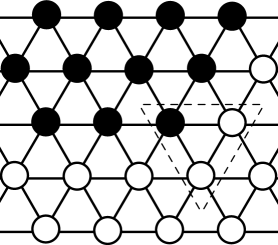
Figure 2: Domain wall kink on the triangular lattice: there is a localized fractional flux $\Phi_{0}/3$ from the plaquette inside the dotted triangle. Here solid (open) circles correspond to spin up (down).

It turns out that the triangular lattice of coupled grains is special in its high degree of order at low temperature. The square lattice for $d\pm id$ grains is at the opposite extreme, as shown in the following section: there is no coupling between the Ising variables and the superconducting phase. The zero-temperature degeneracy for the square lattice is thus given by a global $U(1)$ for the superconducting phase times a factor of 2 per site from the Ising variables.

The case of $p\pm ip$ superconductors on the square lattice is quite complex and is shown below to be connected to the existence of a $\mathbb{Z}_{2}$ topological order. We find that $p\pm ip$ superconductors on the square lattice support localized $\pi$-vortices with half the enclosed flux of an ordinary superconducting vortex, and these vortices drive the superconducting transition.

V Square lattice: deconfinement

Square arrays of both $p+ip$ and $d+id$ superconductors show dramatically different behavior from the triangular lattice discussed above: both have no order of the Ising $T$ variables even at zero temperature when only the Josephson coupling is considered, i.e., only single-Cooper-pair processes are included in the model.

The gauge flux $\Phi_{a}$ that pierces an elementary plaquette in the square lattice is given by

$$\Phi_{a}={k\over 4}({\sigma}_{1}+{\sigma}_{2}+{\sigma}_{3}+{\sigma}_{4})~{}~{}\mod 1.$$ (15)

Again $k=1$ for $p+ip$ and $k=2$ for $d+id$. For $d+id$ the flux generated by the Ising variables is ${1\over 2}\sum_{\square}{\sigma}_{i}$, which is always an integer. Since integer gauge flux can always be gauged away, the problem decouples into a square-lattice XY model and a non-interacting Ising model.

The case of $p+ip$ arrays is more interesting. In this case $\Phi_{a}={1\over 4}\sum_{\square}{\sigma}_{i}$ and hence can be fractional. Indeed, for 0, 2, or 4 up spins per square $\Phi_{a}$ is an integer, while for 1 or 3 up spins $\Phi_{a}$ is $\frac{1}{2}$ plus an integer. In the ground state, the Ising spin configurations must satisfy the constraint that there are even number of up spins in every plaquette. In a system with open boundary conditions and size $M$ by $N$, the number of such Ising configurations is $2^{M}\times 2^{N}$. The first factor corresponds to the number of ways to fix all the spins on one horizontal line, and the second factor the number of ways to fix all the spins on one vertical line. Once those spins are fixed, the remaining spins are uniquely determined by the constraint (Fig. 3). This implies that, although the above system appears two-dimensional, its ground-state entropy grows as the system’s linear size rather than its area.

Figure 3: A typical ground state configuration of Ising variables (open or filled circles) for $p\pm ip$ superconductors. Note that fixing one row and one column determines the rest of the lattice via the constraint of 0, 2, 4 up-spins per square.

The ground-state constraint of 0, 2, or 4 up-spins per square corresponds to a degenerate case of the eight-vertex modelBaxter (1982), which can be mapped onto the six-vertex modelLieb (1967) using a duality transformationFan and Wu (1970). The point described by ${1\over 4}\sum_{\square}{\sigma}_{i}$ integral is quite special: it divides a region of the phase diagram with extensive (two-dimensional) entropy from a region with finite (zero-dimensional) entropy.

The ground states for $p\pm ip$ superconductors on the square lattice are the same as those of the Ising lattice gauge model

$$H=-K\sum_{i,j}\sigma_{(i,j)}\sigma_{(i+1,j)}\sigma_{(i+1,j+1)}\sigma_{(i+1,j)},$$ (16)

since the product around a plaquette takes the value $+1$ for $0,2,4$ up spins, and $-1$ otherwise. A plaquette with $1$ or $3$ up spins generates a gauge flux. Whether such defective plaquettes are entropically confined is equivalent to whether the the $\pi$-gauge flux is confined in the gauge theory when $K\rightarrow 0$. Our previous degeneracy counting implies that the $\pi$ gauge flux would completely deconfined if the entropic term were the only contribution to its free energy. In reality, in addition to the entropic contribution, there is a phase stiffness contribution to the interaction between two fractional gauge flux. Indeed, when $\Phi_{a}$ is a fraction, it cannot be screened by integer vortices $n_{a}$. As the result, two fractional fluxes $\Phi_{a}$ separated by a large distance $R$ cost free energy $\sim(\pi K/4)\log R$, where $K$ is the renormalized phase stiffness. This logarithmic interaction binds half-integer vortices at low temperatures.

The half-integer vortices are relevant at the ordinary (integer vortex) XY transition because their scaling dimension is four times smaller than that of the integer vortices, which are marginal at the transition. It follows that as the temperature is raised above a critical value, the half-integer vortices unbind and the superconductivity is lost. The superconducting phase below this temperature has “nematic” order in that there is long-range order in the square $\psi^{2}$ of the Cooper pair operator, rather than in $\psi$.

A defective plaquette can be viewed as a $\pi$-flux bound to a fractional Ising charge. The Ising charge associated with a given plaquette is defined as

$$Q_{I}={(N_{\uparrow,\square}-2)\over 2},$$ (17)

where $N_{\uparrow,\square}$ is the number of up spins in the plaquette. Any plaquette satisfying the 0, 2, 4 constraint has an integral $Q_{I}$. An isolated plaquette with 1 or 3 up spins has half-integer $Q_{I}$. Since the Josephson energy is only sensitive to whether the $Q_{I}$ is integer or half-integer, one should regard $Q_{I}$ as defined modulo integer since two half-integer $Q_{I}$ cancel. Local constraints like (15) were used inMotrunich and Senthil (2002) to generate a gauge theory, but required a somewhat artificial charging energy that is associated with plaquettes, not with single grains or with long-range interactions. We have shown that geometric phases in Josephson junction arrays naturally generate such a plaquette constraint, and in turn a classical two-dimensional $\mathbb{Z}_{2}$ gauge theory.

VI Honeycomb lattice: criticality

We now study coupled $p\pm ip$ and $d\pm id$ grains on the honeycomb lattice and show that the essential low-temperature physics is considerably modified from the triangular and square cases studied in the preceding sections. This model will be shown to have an extensive entropy down to zero temperature with no macroscopic order of the Ising sign variable. Hence even though locally (i.e. in each superconducting grain) T-breaking superconductivity is favored, globally there is no time-reversal symmetry breaking; there is instead a critical state at zero temperature.

For the honeycomb lattice, the gauge flux in each hexagon is given by

$$\Phi_{a}={k\over 6}({\sigma}_{1}+{\sigma}_{2}+{\sigma}_{3}+{\sigma}_{4}+{\sigma}_{5}+{\sigma}_{6}),~{}~{}\mod 1.$$ (18)

Hence a plaquette with zero, three, or six up-spins has integer $\Phi_{a}$, and does not cause any frustration in the Josephson energy. Thus the lowest energy Ising spin configurations satisfy the 0, 3, 6 constraint in every plaquette. The number of such configurations can be found exactly in the thermodynamic limit by a mappingDi Francesco and Guitter (1994) (section VII) onto the three-color model solved exactly by BaxterBaxter (1970). The result gives an entropy per hexagon equal to $0.379114k_{B}$. The critical properties of this three-color model are briefly reviewed in section VII.

Ising configurations that violate the 0, 3, 6 constraint lead to fractional gauge fluxes. The number of Ising configurations consistent with a distribution of fractional gauge fluxes is different from that of the ground state degeneracy discussed above. The logarithm of the ratio between these degeneracies gives rise to a entropic contribution to the interaction free energy between fractional gauge fluxes. To compute such interaction we need to consider a correlation function that does not have an analogue in the three-color model: this is the main subject of section VII. Here we explore the physical consequences of the entropic interaction.

To be more precise let us return to Eq. (12). For a fixed distribution $\{\Phi_{a}\}$ ($-1/2\leq\Phi_{a}<1/2$) the entropic contribution to the dimensionless free energy is given by

$$e^{-\Delta F(\{\Phi_{a}\})}={\sum_{\{{\sigma}_{j}\}}\prod_{a}{\tilde{\delta}}\Big{(}\Phi_{a}-{k\over 6}\sum_{j\in a}{\sigma}_{j}\Big{)}\over\sum_{\{{\sigma}_{j}\}}\prod_{a}{\tilde{\delta}}\Big{(}{k\over 6}\sum_{j\in a}{\sigma}_{j}\Big{)}}.$$ (19)

Here the function ${\tilde{\delta}}(x)$ is 1 if $x\in\mathbb{Z}$, 0 otherwise. After the summation over the Ising variables, Eq. (12) becomes

$$Z \propto\sum_{\{n_{a}\}}e^{-S(\{n_{a},\Phi_{a}\})},$$ (20)

where

$$S =\Delta_{c}\sum_{a}(n_{a}-\Phi_{a})^{2}+\sum_{a,b}(n_{a}-\Phi_{a})G_{ab}(n_{b}-\Phi_{b})$$ (21)

$$+\Delta F(\{\Phi_{a}\}).$$

The question is what effect, if any, does $\Delta F(\{\Phi_{a}\})$ have on the thermodynamics of the vortices?

Section VII shows that the probability $e^{-\Delta F}$ associated with two $\Phi_{a}=\pm 1/3$ defect plaquettes of opposite fractional flux falls off with distance approximately as $r^{-4/9}$. This implies a free energy cost of

$$\Delta F=4~{}\Phi_{a}\log|r_{a}-r_{b}|\Phi_{b}.$$ (22)

Imagine the stiffness $K$ is tuned so that the system is exactly at the critical point where integer vortices proliferate if fractional vortices are strictly forbidden. Then the vortex fugacity operator is marginal (has scaling dimension 2). From the Gaussian spin-wave theory vortices of fractional charge 1/3 have scaling dimension $\Delta=2/9$. However, this analysis ignores the entropic contribution to the free energy. Including that effect from Eq. (22) implies the total scaling dimension of fractional 1/3 vortices at the (integer vortex unbinding) KT point

$$\Delta=2/9+2/9=4/9.$$ (23)

This indicates that fractional vortices are in fact relevant, and most likely it is their unbinding that drives the superconductor-normal XY-type transition. The superconducting phase is then a “triatic” with long-range order in the cube of the Cooper pair operator $\psi^{3}$ rather than $\psi$.

There are several corrections in realistic systems (quenched disorder, multiple-Cooper-pair processes, etc.) that will split the extensive zero-temperature entropy, as discussed briefly in the final section and in a forthcoming paper by Castelnovo, Pujol, and ChamonCastelnovo et al. . However, these effects can be expected to onset at temperatures much less than the Josephson coupling ($kT\ll E_{J}$), so experiments on the honeycomb lattice at the lowest accessible temperatures are likely to see an extensive entropy and critical correlations of the time-reversal order parameter. The following section obtains these critical properties using the connection to the three-color model.

VII The $T=0$ critical theory on the honeycomb lattice

As shown in section VI, the ground state configurations of the Ising spins have 0, 3, or 6 up-spins on each hexagon. The entropy per site of this “0, 3, 6-model” was earlier shownDi Francesco and Guitter (1994, ) to be equal to that of the “three-color problem” solved by Baxter. In the three-color problem, one assigns one of three colors (say red, green, blue) to each bond of the honeycomb lattice, with the requirement that all three colors meet at each site. A quantity called chirality can be defined in the following way. At each site there are three bonds each being colored differently. Start with the red bond and turn clockwise: if the sequence of colors encountered is RGB we assign chirality ${\sigma}=+1$ to that site. If the sequence is RBG we assign ${\sigma}=-1$. In this way each coloring pattern is uniquely associated with an Ising configuration. The 0, 3, 6 constraint ensures that one returns to the original color after going around a plaquette (hexagon). Since the colors are uniquely determined from the Ising variables once one bond is fixed, the entropy of the two models differs by a global factor of 3. Baxter has shown that the entropy per hexagon is Baxter (1970)

$$S=\log\left({2^{2}\over 1\cdot 3}{5^{2}\over 4\cdot 6}{8^{2}\over 7\cdot 9}\cdots\right)\approx 0.37905.$$ (24)

The three-color model is an example of zero temperature models that have critical correlationsBerker and Kadanoff (1980), and many of its critical properties are known exactly. To determine these properties it is useful to represent the three-color model as a two-component height model (on the dual, triangular, lattice) as followsRead ; Huse and Rutenberg (1992); Kondev and Henley (1996). Consider a given site on one sublattice (say $A$), and the three colored bonds stemming from it. If we cross a given bond in a clockwise fashion with respect to the site, the following increment to the high variable is assigned:

$$\Delta{\bf h} =(1,0)~{}~{}red$$ (25)

$$=(-1/2,\sqrt{3}/2)~{}~{}blue$$

$$=(-1/2,-\sqrt{3}/2)~{}~{}green$$

This assignment is self-consistent since the three-color constraint ensures the total height increment is 0 after one completes a loop. The height increment gets a factor of $-1$ if the crossing is counterclockwise with respect to sublattice $A$. The long-wavelength effective theory for this problem is given by

$$F=\int\left(\frac{K}{2}(\nabla{\bf h})^{2}+V({\bf h})\right)\,d^{2}x,$$ (26)

where the potential $V$ has the periodicity of a honeycomb lattice of side $1/\sqrt{3}$. The stiffness $K$ is determined by the requirement that the locking potential $V$ be marginal.

In this theory the allowed vertex operators have the form ${\hat{O}}_{\bf\alpha}(x)=\exp(i\alpha_{i}h_{i}(x))$ where ${\bf\alpha}$ lies on the reciprocal lattice of $V$. The scaling dimension $\Delta$ of such an operator, which determines its correlations through $\langle{\hat{O}}_{\bf\alpha}(0){\bar{\hat{O}}}_{\bf\alpha}({\bf x})\rangle\sim r^{-2\Delta}$, is given by $\Delta=\alpha^{2}/(3\pi)$. Knowing the critical theory of the three color problem it is possible to compute the entropy associated with certain localized defects in the color assignment. These defects appear as vortex operators; among them the most relevant one has scaling dimension $\Delta=1/2$. This information allows us to determine the full critical three-color theory. This critical theory (26) has a hidden $SU(3)$ symmetryRead . The field-theory representation of the $SU(3)$ symmetry of (26) is given inKondev and Henley (1996).

Unfortunately knowledge about the three-color model does not enable us to compute the entropic contribution to the interaction between fractional gauge fluxes as in Eq. (22). This is because a single plaquette with the wrong number of up Ising spins spoils the mapping to the three-color model. For example, on circling a defect plaquette with only 2 Ising spins, the colors wind up cyclically permuted. To find the entropic interaction between a pair of fractional vortices with opposite vorticity, we numerically computed the ratio in Eq. (19).

We have performed numerical transfer-matrix calculations on strips and cylinders of up to 9 hexagons width/circumference. The entropy for the ground state is calculated as follows: configurations allowed by the constraint (0, 3, or 6 up-spins on each hexagon) are assigned $\beta E=0$, while forbidden configurations have $\beta E=\infty$. Let the length of the strip be $N$: the entropy is given by

$$S=\log Z=\log(T^{N})=N\log\lambda_{1},$$ (27)

where $\lambda_{1}$ is the largest eigenvalue (assumed nondegenerate) of the transfer matrix $T$. The entropy per hexagon of the 2D system, if extensive, can then be estimated as

$$S/\hexagon=\lim_{W\rightarrow\infty}{\log\lambda_{1}(W)\over W},$$ (28)

where $W$ is the width of the strip. Table I shows the resulting estimates with periodic and open boundary conditions for strips of various widths.

Width	Estimated $S/\hexagon$		$\Delta_{d}$	$\Delta_{c}$
	Open	Periodic
1	1.05
2	0.703
3	0.590	$0.462$	0.210
4	0.534
5	0.502
6	0.480	0.403	0.231	1.90
7	0.465
8	0.454
9		0.390	0.235	1.91
$\vdots$	$\vdots$	$\vdots$
Theory ($\infty$)	0.379114	0.379114		2

Table 1: Results of numerical transfer-matrix calculations: estimates of $T=0$ entropy and correlations. The correlation between two defect plaquettes of opposite sign (e.g., one with 2 spins up and one with 4) falls off as $r^{-2\Delta_{d}}$, and the chirality correlation falls off as $r^{-2\Delta_{c}}$.

The transfer matrix can also be used to calculate the entropic interaction between a pair of plaquettes with opposite flux on a cylinder. These defect plaquettes must be on the same sublattice for a nonzero correlation. We use the usual procedureCardy (1996) for extracting scaling dimensions at a critical point from calculations on the cylinder, based on the hypothesis of conformal invariance. The relative probability to have positive and negative defect plaquettes at fixed locations, described by transfer matrices $T_{+}$ and $T_{-}$, separated by $n$ defect-free rings around the cylinder, is

$$p(n)={Z(n)\over Z}=\lim_{N\rightarrow\infty}{{\rm Tr}\ T^{N}T_{+}T^{n}T_{-}T^{N}\over{\rm Tr}\ T^{2N+n+2}}.$$ (29)

If this function in the continuum limit is a correlation function of a critical theory in 2D, then conformal invariance predicts that correlations along the cylinder at large distances $r\gg L$, $L$ the circumference of the cylinder, should fall off as

$$p(r)\sim e^{-r/\xi},\quad\xi={L\over 2\pi\Delta}.$$ (30)

As seen in Table I, this characteristic dependence is indeed observed for both the fractional-vortex-defect correlator and the Ising correlator.

The numerical results suggest that

$$e^{-\Delta F(r_{a},r_{b})}\sim{1\over|r_{a}-r_{b}|^{0.47}}.$$ (31)

This implies that the fractional vortices corresponds to an operator with scaling dimension $\Delta\approx 0.235$ in the 0, 3, 6 model. Since the lowest two scaling dimensions that appear in the three-color model are $\Delta=1/2$ and $\Delta=2/3$ which are very different from $0.235$, it is apparent that the critical theory of the 0, 3, 6 model has a different operator content than the three-color model.

Such a critical theory must have the same correlators of height variables as the three-color model, and yet have a different set of defect operators, including the defective plaquette with $\Delta\approx 0.23$. One possibility is the “orbifold” dual of the above three-color model theory obtained by identifying heights that differ by a $\mathbb{Z}_{3}$ transformation $h_{1}+ih_{2}\rightarrow\exp(2i\pi n/3)(h_{1}+ih_{2})$. The physical significance of this identification is that the fractional vortices, around which the height lattice is rotated by $2\pi/3$, are now allowed defects. On the torus, there are now different sectors of the theory corresponding to how the color scheme is shifted upon passing from one boundary of the torus to another. We find that the orbifold “twist” operators that connect these different sectorsDulat and Wendland (2000) have scaling dimension 2/9 and may correspond to the fundamental plaquette defects in the 0, 3, 6-model. However, this identification is quite indirect at present and should be regarded as only one of several possibilities for the critical theory. This orbifolded $SU(3)$ theory with $c=2$ has previously been considered as a hypothetical model of a quantum Hall edgeSkoulakis and Thomas (1999), since the non-orbifolded $SU(3)$ theory describes several real quantum Hall edgesKane and Fisher (1994); Moore and Wen (1998) in the chiral Luttinger liquid approachWen (1992).

Finally, Eq. (31) indicates that fractional vortices have already become unbound when the integer vortex pairs disassociate. To see that we imagine forbidding the fractional vortices and tuning the stiffness constant $K$ so that the integer vortex just about to unbind. At that point the vortex fugacity operator is marginal (has scaling dimension 2), and 1/3 vortices have scaling dimension $\Delta_{i}=2/9$. Adding the entropic interaction (Eq. (31)) this yields the total scaling of the fractional vortex fugacity operator

$$\Delta=\Delta_{i}+\Delta_{e}=2/9+2/9=4/9.$$ (32)

This indicates that fractional vortices are in fact relevant, and most likely it is their unbinding that drives the superconductor-normal XY-type transition. The superconducting state has “triatic” order in $\psi^{3}$ rather than in $\psi$, as in the ground state of the antiferromagnetic XY model on the kagomé latticeHuse and Rutenberg (1992).

VIII Summary and other directions: dynamics and quenched disorder

Our main goal in this paper was to demonstrate that due to the coupling of the order parameter and the underlying crystalline lattice, Josephson junction arrays made of time-reversal-symmetry- breaking superconductors exhibit very much richer physics than their $s$ or $d$ counterparts. Phase-sensitive experiments such as those in Ref.Tsuei et al. (1994); Wollman et al. (1993) should be able to detect the variable tunneling phases caused by a $T$-breaking order parameter. Regular arrays of such grains give rise to realizations of Higgs-gauge models, and are new examples of topological order with deep connections to frustrated magnets. The ordering of the time-reversal order parameter and the onset of superconductivity depends intricately on the geometry of the arrays.

One can expect, on a qualitative level, that the existence of the nontrivial phases studied above will also modify the behavior in random polycrystalline samples. The behavior in the random case is likely quite complex since random Josephson coupling, even without the gauge phases we have studied, leads to the “dirty boson” problemFisher (1990); Vishwanath et al. . Allowing random local orientation of the order parameter for $d$ superconductors has been argued to induce a superparamagnetism effectSigrist and Rice (1995) that will coexist with the spontaneous orbital currents in the $d+id$ case. A more tractable model would be to allow a quenched time-reversal-symmetry breaking field coupling to the Ising variables, but keep uniform the strength of the Josephson coupling.

The possibility of a direct coupling between the Ising variables at higher order in the Josephson tunneling is studied in a forthcoming paperCastelnovo et al. . This model has phase transitions from the critical phase with no additional interaction to ordered ferromagnetic and antiferromagnetic phases. Its dynamics are of special interest, as the three-color model has previously been studied as a model system for glassy dynamicsChakraborty et al. (2002). Our realization of the three-color model in arrays of complex superconducting grains may prove to be experimentally less challenging than recent effortsPark and Huse (2001) to build frustrated XY models on the kagomé lattice using $s$ superconductors and a frustrating magnetic field.

IX acknowledgements

J. E. M. acknowledges helpful discussions and correspondence with C. Chamon, P. Fendley, O. Ganor, J. Kondev, and S. Thomas, and the hospitality of the Aspen Center for Physics. The authors were supported by NSF DMR-0238760 and the Hellman Foundation (J. E. M.), and DOE (D. H. L.). This research used resources of the National Energy Research Scientific Computing Center, supported by DOE contract DE-AC03-76SF00098.

References

- Takada et al. (2003) K. Takada, H. Sakurai, E. Takayama-Muromachi, F. Izumi, R. A. Dilanian, and T. Sasaki, Nature 422, 53 (2003).
- Baskaran (2003) G. Baskaran, Phys. Rev. Lett. 91, 097003 (2003).
- (3) Q. H. Wang, D. H. Lee, and P. A. Lee, eprint cond-mat/0304377.
- (4) B. Kumar and S. Shastry, eprint cond-mat/0304210.
- Mackenzie and Maeno (2003) A. P. Mackenzie and Y. Maeno, Rev. Mod. Phys. 75, 657 (2003).
- Tsuei et al. (1994) C. C. Tsuei, J. R. Kirtley, C. C. Chi, L. S. Yu-Jahnes, A. Gupta, T. Shaw, J. Z. Sun, and M. B. Ketchen, Phys. Rev. Lett. 73, 593 (1994).
- Wollman et al. (1993) D. A. Wollman, D. J. Van Harlingen, W. C. Lee, D. M. Ginsberg, and A. J. Leggett, Phys. Rev. Lett. 71, 2134 (1993).
- Ioffe and Feigel’man (2002) L. B. Ioffe and M. V. Feigel’man, Phys. Rev. B 66, 224503 (2002).
- (9) B. Doucot, L. B. Ioffe, and J. Vidal, eprint cond-mat/0302104.
- (10) P. Henelius, A. V. Balatsky, and J. R. Schrieffer, eprint cond-mat/0004413.
- Sigrist and Ueda (1991) M. Sigrist and K. Ueda, Rev. Mod. Phys. 63, 239 (1991).
- Senthil and Fisher (2000) T. Senthil and M. P. A. Fisher, Phys. Rev. B 62, 7850 (2000).
- Moessner and Sondhi (2001) R. Moessner and S. Sondhi, Phys. Rev. Lett. 86, 1881 (2001).
- Baxter (1970) R. J. Baxter, J. Math. Phys. 11, 784 (1970).
- Chalker et al. (1992) J. T. Chalker, P. C. W. Holdsworth, and E. F. Shender, Phys. Rev. Lett. 68, 855 (1992).
- (16) N. Read, eprint Kagomé workshop, unpublished (1992).
- (17) C. L. Henley, eprint unpublished (1992).
- Huse and Rutenberg (1992) D. A. Huse and A. D. Rutenberg, Phys. Rev. B 45, 7536 (1992).
- Chandra et al. (1993) P. Chandra, P. Coleman, and I. Ritchey, J. de Phys. I 3, 591 (1993).
- (20) eprint The order parameter given in Eq. (5) has the same symmetry under rotations by a multiple of as the explicit form found from mean-field RVB for the triangular lattice, although the triangular-lattice form does not have the full continuous rotational symmetry. In general, when considering lattices of grains, our results will apply without modification as long as the crystal-field modification of the order parameter within each grain is compatible with the lattice of grains.
- Kosterlitz and Thouless (1973) J. M. Kosterlitz and D. J. Thouless, J. Phys. C 6, 1181 (1973).
- José et al. (1977) J. V. José, L. P. Kadanoff, S. Kirkpatrick, and D. R. Nelson, Phys. Rev. B 16, 1217 (1977).
- Lee et al. (1986) D. H. Lee, G. Grinstein, and J. Toner, Phys. Rev. Lett. 56, 2318 (1986).
- Baxter (1982) R. J. Baxter, Exactly solved models in statistical mechanics (Academic Press, London, 1982).
- Lieb (1967) E. H. Lieb, Phys. Rev. 162, 162 (1967).
- Fan and Wu (1970) C. Fan and F. Y. Wu, Phys. Rev. B 2, 723 (1970).
- Motrunich and Senthil (2002) O. I. Motrunich and T. Senthil, Phys. Rev. Lett. 89, 277004 (2002).
- Di Francesco and Guitter (1994) P. Di Francesco and E. Guitter, Europhys. Lett. 26, 455 (1994).
- (29) C. Castelnovo, P. Pujol, and C. Chamon, eprint unpublished.
- (30) P. Di Francesco and E. Guitter, eprint cond-mat/9406041.
- Berker and Kadanoff (1980) A. N. Berker and L. P. Kadanoff, J. Phys. A 13, L259 (1980).
- Kondev and Henley (1996) J. Kondev and C. L. Henley, Nucl. Phys. B 464, 540 (1996).
- Cardy (1996) J. L. Cardy, Scaling and renormalization in statistical physics (Cambridge, 1996).
- Dulat and Wendland (2000) S. Dulat and K. Wendland, JHEP 6, 012 (2000).
- Skoulakis and Thomas (1999) S. Skoulakis and S. Thomas, Nucl. Phys. B 538, 659 (1999).
- Kane and Fisher (1994) C. L. Kane and M. P. A. Fisher, Phys. Rev. B 51, 13449 (1994).
- Moore and Wen (1998) J. E. Moore and X.-G. Wen, Phys. Rev. B 57, 10138 (1998).
- Wen (1992) X.-G. Wen, Int. J. Mod. Phys. B 6, 1711 (1992).
- Fisher (1990) M. P. A. Fisher, Phys. Rev. Lett. 65, 923 (1990).
- (40) A. Vishwanath, J. E. Moore, and T. Senthil, eprint cond-mat/0209109.
- Sigrist and Rice (1995) M. Sigrist and T. M. Rice, Rev. Mod. Phys. 67, 503 (1995).
- Chakraborty et al. (2002) B. Chakraborty, D. Das, and J. Kondev, Eur. Phys. J. E 9, 227 (2002).
- Park and Huse (2001) K. Park and D. A. Huse, Phys. Rev. B 64, 134522 (2001).