Coulomb Effects in Tunneling through a Quantum Dot Stack

Abstract

Tunneling through two vertically coupled quantum dots is studied by means of a Pauli master equation model. The observation of double peaks in the current-voltage characteristic in a recent experiment is analyzed in terms of the tunnel coupling between the quantum dots and the coupling to the contacts. Different regimes for the emitter chemical potential indicating different peak scenarios in the tunneling current are discussed in detail. We show by comparison with a density matrix approach that the interplay of coherent and incoherent effects in the stationary current can be fully described by this approach.

I Introduction

Resonant tunneling through coupled quantum dots (QDs) is an active field of theoretical and experimental research (for a recent review see van der Wiel et al. (2003)). Various nano-scale geometries for double QD systems were under investigation: lateral gate-defined devices (e.g. in Ref. van der Vaart et al. (1995)) or vertical mesa structures as proposed in Ref. Klimeck et al. (1994). With the recent advances in fabrication of stacked self-organized QDs where only few stacks can be selected by electronic transport measurements an ideal system for studying “artificial molecules” was developed Borgstrom et al. (2001); Bryllert et al. (2002, 2003). The current-voltage characteristic of such a double QD stack can show peaks with very high peak-to-valley ratio Borgstrom et al. (2001) due to the sharp energetic resonance condition of levels in different QDs. In Ref. Borgstrom et al. (2001) the authors also report on the frequent observation of double peaks in the tunneling current which they relate to the effect of Coulomb interaction. In the present paper, we give a detailed theoretical examination of this experimental feature and we analyze the mechanisms of the current peak broadening and height. We use a Pauli master equation model where the tunneling to the contacts is treated by tunneling rates and the coupling between the QDs is described by Fermi’s golden rule. The result of this treatment for the stationary current through noninteracting QDs is in agreement with recent density matrix calculations. We will show that the occurrence of double peaks in the current depends on the emitter chemical potential, on the tunneling rates, and on the Coulomb interaction strength of electrons inside the QD as well as in different QDs. Different scenarios corresponding to different parameter regimes will be considered.

The outline of the paper is as follows: in Sec. II we introduce the model based on a Pauli master equation; in Sec. III we present the analytical and numerical results for the stationary current through the double QD stack, followed by a discussion. In particular, this section is subdivided into the case of noninteracting electrons (Sec. III.1) where we discuss the effect of current peak broadening and height, and into the case of Coulomb interacting electrons (Sec. III.2) where double current peaks under certain conditions occur; conclusions are drawn in Sec. IV.

II Model

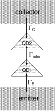
Figure 1: Scheme of the quantum dot stack connected to emitter/collector contact with tunneling rates $\Gamma_{E/C}$, respectively, and tunneling rate $\Gamma_{\mathrm{inter}}$ between the quantum dots.

In Fig. 1 the double QD system is sketched: QD1 is connected to an emitter contact with a tunneling rate $\Gamma_{E}$, QD2 is connected to a collector contact with a tunneling rate $\Gamma_{C}$, and both QDs are tunnel coupled mutually with a rate $\Gamma_{\mathrm{inter}}$ (for the definition see below). We consider one spin degenerate single-particle state per QD. The many-particle (Fock-) states $\nu$ of the QD stack are characterized by occupation numbers $n_{is}^{(\nu)}\in\{0,1\}$, where $i=1,2$ labels the QD and $s=\uparrow,\downarrow$ labels the spin degree of freedom. Thus $\nu=(n_{1\uparrow}^{(\nu)},n_{1\downarrow}^{(\nu)},n_{2\uparrow}^{(\nu)},n_{2\downarrow}^{(\nu)})$ gives 16 different Fock states.

The emitter/collector contact is assumed to be in local equilibrium characterized by Fermi functions $n_{F}^{E/C}(E)=1/(1+\exp((E-\mu_{E/C})/k_{B}T))$ with chemical potentials $\mu_{E/C}$, respectively, and temperature $T$. An applied bias voltage $V=(\mu_{E}-\mu_{C})/e$ drives the QD system out of equilibrium. Throughout the calculations we choose the sign of the elementary charge $e>0$ so that $V>0$ means $\mu_{E}>\mu_{C}$ and $I>0$ describes a net particle current from emitter to collector. The single-particle energies $E_{i}$ in the QDs are assumed to shift linearly with respect to the bias voltage $V$: $E_{i}(V)=E_{i}-e\eta_{i}V$ with the leverage factor $\eta_{i}$ for the $i$-th QD. The total energy of the state $\nu$ is

$$E(\nu)=\sum_{i=1}^{2}N_{i}(\nu)(E_{i}-e\eta_{i}V)+U(\nu)$$ (1)

where $N_{i}(\nu)=n_{i\uparrow}^{(\nu)}+n_{i\downarrow}^{(\nu)}$ is the particle number of the $i$-th QD for state $\nu$ and $U(\nu)$ is the charging energy for state $\nu$ which is given by Beenakker (1991); Kießlich et al. (2002a, b); Kießlich et al. (2003)

$$U(\nu)=\frac{e^{2}}{2}\sum_{i,j}N_{i}(\nu)\left[C^{-1}\right]_{ij}N_{j}(\nu)\\ -\frac{e^{2}}{2}\sum_{i}\left[C^{-1}\right]_{ii}N_{i}(\nu)$$ (2)

with the inverse of the capacitance matrix $C$, where the last term subtracts the self-interaction.

The evolution of the system is described by the Pauli master equation

$$\frac{d}{dt}\underline{P}=\underline{\underline{M}}\cdot\underline{P}$$ (3)

for the occupation probabilities $\underline{P}=(\{P_{\nu}\})^{T}$. The matrix $\underline{\underline{M}}$ contains the transition rates $M_{\nu\nu^{\prime}}$ between the Fock states $\nu^{\prime}\to\nu$. Confining attention to single particle transitions all elements $M_{\nu\nu^{\prime}}$ are zero if the total particle number $N(\nu)=\sum_{i}N_{i}(\nu)$ differs by more than one from $N(\nu^{\prime})$. For a transition which increases the total particle number by unity, i.e. an electron enters the QD stack via the emitter/collector barrier, respectively, the transition rate reads $M_{\nu\nu^{\prime}}=\Gamma_{E/C}n_{F}^{E/C}(\Delta E_{\nu\nu^{\prime}})$ where $\Delta E_{\nu\nu^{\prime}}=E(\nu)-E(\nu^{\prime})$ is the difference of total energies. For the inverse tunneling processes the transition rate is $M_{\nu\nu^{\prime}}=\Gamma_{E/C}(1-n_{F}^{E/C}(\Delta E_{\nu^{\prime}\nu})$). Transitions which do not change the total particle number describe tunneling between QD1 and QD2: Taking into account the broadening of the transition due to the finite lifetime in the quantum dots, Fermi’s golden rule provides us with

$$\begin{split}M_{\nu\nu^{\prime}}=&2\pi|\Omega|^{2}\left[\frac{1}{\pi}\frac{\Gamma/2}{(\Delta E_{\nu\nu^{\prime}})^{2}+(\Gamma/2)^{2}}\right]\\ =&\Gamma_{\mathrm{inter}}\,L(\Delta E_{\nu\nu^{\prime}},\Gamma)\end{split}$$ (4)

Here $\Omega$ is the tunneling matrix element and $\Gamma\equiv\Gamma_{E}+\Gamma_{C}$. The maximum tunneling rate is $\Gamma_{\mathrm{inter}}=4|\Omega|^{2}/\Gamma$ and $L(x,w)\equiv(1+(2x/w)^{2})^{-1}$ is a Lorentzian function in $x$ with a FWHM of $w$. For convenience we measure rates and energies in the same units here, i.e. setting $\hbar=1$.

Throughout this paper we investigate the steady state current so that the stationary occupation probabilities $P_{\nu}^{0}$ evaluated by $\underline{\underline{M}}\cdot\underline{P}^{0}=0$ are used. In this case the current can be evaluated by counting the tunneling events over the collector barrier. Summing the corresponding transitions probabilities we find

$$I=\sum_{\nu,\nu^{\prime}}eM_{\nu^{\prime}\nu}\left(1-\delta_{N(\nu)N(\nu^{\prime})}\right)(N_{2}(\nu)-N_{2}(\nu^{\prime}))P_{\nu}^{0}$$ (5)

where the additional factors ensure that the tunneling process occurs at the collector barrier and the correct sign is taken into account for the current direction.

III Discussion and Results

III.1 Noninteracting quantum dots: Current peak width and height

If the energies of single-particle states in two different QDs are resonant, a current flows through the QD stack and a peak arises in the current-voltage characteristic. In this section we give an analytical derivation of the current for noninteracting QDs, i.e. setting $U(\nu)\equiv 0$ in Eq. (1). Then both spin directions decouple and we can restrict ourselves to a single spin direction here. For the single-particle levels in QD1 and QD2 it is assumed that $E_{1}-\mu_{E}\gg k_{B}T$ and $\mu_{C}-E_{2}\gg k_{B}T$ such that $n_{F}^{E}\approx$1 and $n_{F}^{C}\approx$0. With $\underline{P}^{0}=(P_{(0,0)}^{0},P_{(1,0)}^{0},P_{(0,1)}^{0},P_{(1,1)}^{0})^{T}$ the matrix $\underline{\underline{M}}$ simply reads

$$\underline{\underline{M}}=\left(\begin{array}[]{cccc}-\Gamma_{E}&\Gamma_{C}&0&0\\ 0&-(\Gamma_{E}+\Gamma_{C}+Z)&Z&0\\ \Gamma_{E}&Z&-Z&\Gamma_{C}\\ 0&\Gamma_{E}&0&-\Gamma_{C}\end{array}\right)$$ (10)

with $Z\equiv\Gamma_{\mathrm{inter}}L(\Delta E_{(1,0)(0,1)},\Gamma)$. The stationary master equation can be rewritten in a rate equation for the occupation numbers $n_{1}$ and $n_{2}$ which results in the following stationary solution

$$\left(\begin{array}[]{c}n_{1}\\ n_{2}\end{array}\right)=\frac{\Gamma_{E}}{\Gamma_{E}\Gamma_{C}+\Gamma Z}\left(\begin{array}[]{c}\Gamma_{C}+Z\\ Z\end{array}\right)$$ (15)

The current (5) then becomes

$$I=e\left[\frac{1}{\Gamma_{E}}+\frac{1}{\Gamma_{C}}+\frac{1}{Z}\right]^{-1}$$ (16)

which can be physically interpreted quite easily: the three barriers in the QD stack act as a series connection of resistors corresponding to the inverse of tunneling rates. After a straightforward transformation of (16) one obtains

$$I=e\Gamma_{w}\,L\left(\Delta E,\Gamma\sqrt{1+\frac{4|\Omega|^{2}}{\Gamma_{E}\Gamma_{C}}}\right)$$ (17)

with $\Gamma_{w}\equiv\left[\frac{1}{\Gamma_{E}}+\frac{1}{\Gamma_{C}}+\frac{1}{\Gamma_{\mathrm{inter}}}\right]^{-1}$. Due to the assumption of a linear dependence of the single-particle levels on the bias voltage it follows for the energy difference $\Delta E=E_{1}-e\eta_{1}V-(E_{2}-e\eta_{2}V)=e(\eta_{2}-\eta_{1})(V-V_{R})$ with the bias voltage for the resonance $eV_{R}\equiv\frac{E_{2}-E_{1}}{\eta_{2}-\eta_{1}}$. Substituting this in Eq. (17) leads to

$$I(V)=e\Gamma_{w}\,L\left(V-V_{R},\frac{\Gamma}{e(\eta_{2}-\eta_{1})}\sqrt{1+\frac{4|\Omega|^{2}}{\Gamma_{E}\Gamma_{C}}}\right)$$ (18)

As expected, the current-voltage characteristic shows a Lorentzian peak at the bias voltage $V_{R}$. Interestingly, its broadening is not just given by the tunneling coupling to the contacts $\Gamma$, but by a line width modified by the correction factor $\sqrt{1+\frac{4|\Omega|^{2}}{\Gamma_{E}\Gamma_{C}}}$. This factor provides a significant increase of the FWHM for the current peak if the tunneling matrix element $|\Omega|$ is larger than the geometric mean $\sqrt{\Gamma_{E}\Gamma_{C}}$ of the contact tunneling rates.

The expression (17) for the stationary current was also found in Gurvitz and Prager (1996); Gurvitz (1998); Wegewijs and Nazarov (1999) where a density matrix approach was used. In the Appendix A we show that both approaches give identical results in the stationary state if electron-electron interaction is neglected.

To discuss Eq. (18) let us assume that $\Gamma_{C}>|\Omega|>\Gamma_{E}$: the current is limited by the lowest rate $\Gamma_{\mathrm{inter}}L(\Delta E,\Gamma)$ for bias voltages $V$ far away from $V_{R}$. If the bias approaches $V_{R}$ this rate is increased until it equals the emitter coupling $\Gamma_{E}$. Now, the emitter barrier starts to limit the current, i.e. the current flattens close to the resonance so that the FWHM value of the current is reached for larger distances from the resonance voltage $V_{R}$. The smaller the ratio of $\Gamma_{E}/|\Omega|$ the broader the current peak.

The peak (maximum) current is given by $I(V_{R})=e\Gamma_{w}$. It has a non-monotonic dependence on the collector tunneling rate $\Gamma_{C}$: for weak collector coupling the peak current increases linearly, it shows a maximum at $\Gamma_{C}=2|\Omega|$ and drops as $1/\Gamma_{C}$ for strong collector coupling. (The same holds for the emitter coupling.) On the basis of the coherent description this was interpreted in Ref. Wegewijs and Nazarov (1999) as a competition between enhanced tunneling for weak collector coupling and destructive interference in the opposite limit. Hence, it is worth to note that one obtains the same effect in a Fermi’s golden rule treatment where no interference is taken into account for. In this picture increasing $\Gamma_{C}$ enhances the transport over the collector barrier but limits the transport between the dots by broadening the transition.

III.2 Coulomb interacting quantum dots

Now, our considerations will be extended to the realistic situation of Coulomb interacting electrons. We describe the interaction of electrons inside QD1 and QD2 with charging energies $e^{2}[C^{-1}]_{11}=U_{1}$ and $e^{2}[C^{-1}]_{22}=U_{2}$, respectively. The Coulomb interaction strength of electrons in different QDs is given by $e^{2}[C^{-1}]_{12}=U_{\mathrm{inter}}$.

III.2.1 Dependence on emitter Fermi energy

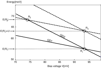
Figure 2: Linear bias voltage dependence of the single-particle energy levels in QD1 ($\eta_{1}=$0.26, $E_{1}=$79.5 meV) and in QD2 ($\eta_{2}=$0.68, $E_{2}=$118.7 meV). Dashed lines: addition energies for the second electron ($U=U_{1}=U_{2}=$8meV, $U_{\mathrm{inter}}=$0).

In Fig. 2 the bias voltage dependence of the QD energies are depicted. The zero-bias single-particle energies $E_{i}$ and leverage factors $\eta_{i}$ were obtained from the calculation of the transmission through a two-dimensional geometry as depicted in Fig. 1 without scattering processes Sprekeler ((2003). In order to describe the experiment, we use the geometry in Ref. Bryllert et al. (2003) which gives $\eta_{1}=$0.26, $E_{1}=$79.5 meV, and $\eta_{2}=$0.68, $E_{2}=$118.7 meV.

Due to the different slopes, the single-particle levels of QD1 and QD2 (full lines in Fig. 2) intersect at the point $R_{1}$. Further resonances can occur by considering the double occupancy of the QDs. Assuming equal charging energies for both QDs ($U=U_{1}=U_{2}=$ 8meV) parallel lines with the additional charging energy $U$ emerge (dashed lines in Fig. 2). The resonance $R_{2}$ is due to the intersection of the energies of the doubly occupied QD1 and the singly occupied QD2. The resonance of the doubly occupied states $R_{3}$ occurs at the same bias voltage as for $R_{1}$ if the charging energies for both QDs are equal.

Figure 3: Contour plot: current I vs. emitter chemical potential $\mu_{E}$ and bias voltage $V$ for $U=U_{1}=U_{2}=$ 8meV, $U_{\mathrm{inter}}=$ 0, $\Gamma_{E}=\Gamma_{C}=$ 100$\mu$eV, $|\Omega|=$10$\mu$eV, $T=4.2$ K. (Isolines correspond to 0.2, 0.4, 0.8 nA)

A current flow through the QD system is possible at the resonance energies $E(R_{1})$ and $E(R_{2})$ providing that electron states in the emitter contact are occupied at these energies. (Typically, these resonances occur at energies far above the chemical potential of the collector Fermi, so that the electrons can always leave the QD system via the collector barrier.) In Fig. 3 the dependence of the current on the emitter chemical potential $\mu_{E}$ and the bias voltage $V$ is shown as a contour plot. Here we assume that the tunnel coupling between the dots is rather weak, i.e. $|\Omega|\ll\Gamma_{E},\Gamma_{C}$, so that the occupation of the dots is determined by the respective reservoirs. The conduction band edge in the emitter is the zero-point of the energy scale. Different scenarios for the stationary current depending on $\mu_{E}$ arise:

• $\mu_{E}<E(R_{1})$: there is only an exponential small current due to thermal activated electrons in the emitter.

• $E(R_{1})<\mu_{E}<E(R_{1})+U=E(R_{3})$: in this case the current shows a peak due to the resonance $R_{1}$ of the single-particle levels, the second resonance $R_{2}$ is energetically available for thermally activated electrons from the emitter and gives rise to an additional current peak at lower bias voltage which increases with increasing temperature (this scenario was experimentally investigated in Bryllert et al. (2003) and was used to determine the charging energy $U$).

• $E(R_{1})+U<\mu_{E}<E(R_{2})$: no current peak appears. In this regime it is possible to add a second electron in QD1. Since the coupling between the QDs is weaker than the coupling to the emitter contact, QD1 is mostly occupied with two electrons. They leave QD1 with the energy $E_{1}+U$ so that they cannot fulfill the resonance condition for $R_{1}$.

• $\mu_{E}>E(R_{2})$: a current peak due to the resonance $R_{2}$ occurs with twice the peak height than in the case (ii) because two electrons contribute to the current here. A current peak for resonance $R_{1}$ is suppressed for the same reasons as in (iii).

III.2.2 Dependence on tunnel coupling

Now we want to study the behavior with increasing tunnel coupling $|\Omega|$. In particular we consider the regime (iv) of the last section but now we allow the tunneling rates to the contacts to be different ($\Gamma_{E}=$ 17$\mu$eV, $\Gamma_{C}=$ 400$\mu$eV).

Figure 4: Current I vs. bias voltage $V$ for varying coupling between QDs $|\Omega|$. $\Gamma_{E}=$ 17$\mu$eV, $\Gamma_{C}=$ 400$\mu$eV, $T=$ 4.2K, $U=U_{1}=U_{2}=$ 8meV, $U_{\mathrm{inter}}=$ 0, $\mu_{E}=$ 90meV

Fig. 4 shows the bias voltage dependent current for varying couplings $|\Omega|$ between the QDs. For low $|\Omega|$ one observes a current peak at $V=$ 75mV corresponding to the resonance $R_{2}$ in Fig. 2 (compare regime (iv) in the last section). According to Eq. (18) the current peak broadens with increasing $|\Omega|$ but one has to consider the double occupancy of QD1 which modifies the current peak width such that the correction factor becomes now $\sqrt{1+2\cdot\frac{4|\Omega|^{2}}{\Gamma_{E}\Gamma_{C}}}$. With increasing $|\Omega|$ a second current peak at the bias voltage of $R_{1}$ appears in Fig. 4. Due to the stronger coupling between the QDs single occupancy of QD1 becomes more likely, since the second electron in QD1 can tunnel into QD2 off-resonantly because of the finite linewidth of the levels. Hence, electrons with energy $E_{1}$ can leave QD1 and contribute in resonance $R_{1}$ which generates a current peak at $V(R_{1})$. Hence, the possibility of the observation of a double current peak in the experiment depends mainly on the tunnel matrix element $\Omega$ between states in different QDs. Its sensitivity on the spatial separation of the QDs within the stack could explain the frequent observation of the double current peaks Borgstrom et al. (2001).

Note that for $|\Omega|\geq$ 260$\mu$eV a small third current peak at almost 110 mV appears due to the resonance of the energies of the doubly occupied QD2 and single occupied QD1 (out of the bias range depicted in Fig. 2).

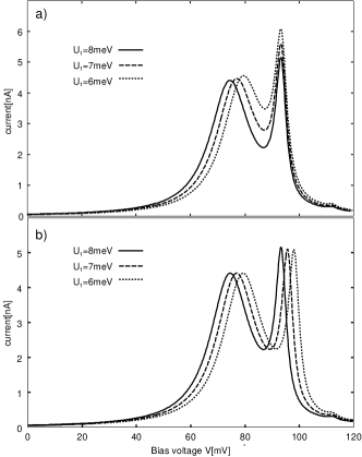
Figure 5: Current I vs. bias voltage $V$ for different charging energies $U_{1}$ of QD1; $U_{2}=$ 8meV; a) $\Gamma_{E}=$ 17$\mu$eV, $\Gamma_{C}=$ 400$\mu$eV; b) $\Gamma_{E}=$ 400$\mu$eV, $\Gamma_{C}=$ 17$\mu$eV; other parameters are the same as for the full curve in Fig. 4

Underlining the corresponding mechanisms which lead to the current peaks in Fig. 4 we show the current-voltage characteristics for different charging energies $U_{1}$ with fixed $U_{2}=$ 8meV in Fig. 5a (the other parameters are the same as for the full curve in Fig. 4). As one can see, with decreasing $U_{1}$ the low bias current peak shifts to higher bias voltages and the second current peak remains at the same bias voltage position: Reducing $U_{1}$ leads to a parallel shift of the dashed line with smaller slope in Fig. 2 so that the intersection point $R_{2}$ shift to higher bias voltages and the resonance $R_{1}$ leaves unchanged. In Fig. 5b the values of $\Gamma_{E}$ and $\Gamma_{C}$ were interchanged so that a different physical situation emerges. Here, both current peaks shift to higher bias voltages by the same amount with decreasing $U_{1}$, i.e. the resonance $R_{3}$ is now mainly responsible for the current peak at higher bias voltage. Due to the weaker collector coupling the double occupancy of both QDs becomes more likely.

Note, that for equal charging energies in QD1 and QD2 the current-voltage characteristics are invariant with respect to an interchange of $\Gamma_{E}$ and $\Gamma_{C}$. This is due to the electron-hole symmetry in the considered QD system. The necessary condition for this symmetry is that the resonances occur at energies deep in the Fermi sea on one contact side and unoccupied states on the other side.

III.2.3 Coulomb interaction between quantum dots

The self-organized QDs within one stack grown in Borgstrom et al. (2001); Bryllert et al. (2002, 2003) have a spatial separation of few nm so that the Coulomb interaction between electrons in different QDs is a crucial ingredient in a theoretical examination. For different interaction strengths $U_{\mathrm{inter}}=$ 0, 2, 4meV the current vs. bias voltage is shown in Fig. 6.

Figure 6: Current I vs. bias voltage $V$ for different Coulomb interaction strengths between QD1 and QD2: $U_{\mathrm{inter}}$, other parameters are the same as for the full curve in Fig. 4

Again a double peak appears whereas the distance of the maxima diminishes with increasing $U_{\mathrm{inter}}$. If QD1 is filled with one electron the single-particle level of QD2 is shifted by $U_{\mathrm{inter}}$ so that the low-bias resonance $R_{2}$ moves to higher bias voltages. The resonance $R_{1}$ stays at the same bias voltage since QD2 filled with one electron generates a shift of the single-particle level of QD1 by the same amount $U_{\mathrm{inter}}$. This gives for the current peak separation

$$\Delta V=\frac{U-U_{\mathrm{inter}}}{e(\eta_{2}-\eta_{1})}$$ (19)

Another feature can be seen in the dotted curve in Fig. 6: if $\Delta V$ becomes smaller, the height of the high-bias peak increases. This peak structure is quite similar to that observed in Borgstrom et al. (2001).

IV Conclusions

The non-equilibrium current-voltage characteristic of a system of two QDs coupled in series was investigated by a Pauli master equation approach. The different leverage factors of the energy levels in the QDs leads to resonances at certain bias voltages. If the emitter contact provides electrons at the resonances a current through the QD system is driven. The height and the width of the arising current peaks in the current voltage characteristic was examined analytically for the case of vanishing Coulomb interaction. Here it was found that the width of the resonance increases if the tunnel coupling between the QDs surpasses the geometric mean of the couplings to the contacts. These results are in full agreement with a fully coherent approach. Including the Coulomb interaction a double current peak can arise for asymmetric coupling to the contacts and a tunnel coupling of the order of the Coulomb interaction strengths. The strong sensitivity of the coupling parameters to the barrier thicknesses in self-organized QD stacks can provide a possible explanation of the frequent observation of double current peaks in the experiment.

Appendix A Derivation of the master equation from density matrix approach

We start with the modified Liouville equation for the double QD system (Fig. 1) derived in Ref. Gurvitz and Prager (1996). The following abbreviations for the Fock states $|\nu\rangle$ will be used: $|a\rangle\equiv|0,0\rangle$, $|b\rangle\equiv|1,0\rangle$, $|c\rangle\equiv|0,1\rangle$, and $|d\rangle\equiv|1,1\rangle$. Then the time evolution of the corresponding density-matrix elements is given by

$$\dot{\rho}_{aa} = -\Gamma_{E}\rho_{aa}+\Gamma_{C}\rho_{cc}$$

$$\dot{\rho}_{bb} = \Gamma_{E}\rho_{aa}+\Gamma_{C}\rho_{dd}+i\Omega(\rho_{bc}-\rho_{cb})$$

$$\dot{\rho}_{cc} = -\Gamma\rho_{cc}-i\Omega(\rho_{bc}-\rho_{cb})$$

$$\dot{\rho}_{dd} = -\Gamma_{C}\rho_{dd}+\Gamma_{E}\rho_{cc}$$

$$\dot{\rho}_{bc} = i\Delta E\rho_{bc}+i\Omega(\rho_{bb}-\rho_{cc})-\frac{1}{2}\Gamma\rho_{bc}$$ (20)

with $\Delta E\equiv E_{2}-E_{1}$ and $\Gamma\equiv\Gamma_{E}+\Gamma_{C}$. Additionally, probability conservation is demanded: $\sum_{\nu}\rho_{\nu\nu}=1$ and $\rho_{cb}=\rho_{bc}^{*}$ holds. Eq. (20) can be transformed in a matrix equation of the form $\dot{\underline{u}}=\underline{\underline{A}}\cdot\underline{u}$ with $\underline{u}\equiv\left(\rho_{aa},\rho_{bb},\rho_{cc},\rho_{dd},\textrm{Re}(\rho_{bc}),\textrm{Im}(\rho_{bc})\right)^{T}$ and

$$\underline{\underline{A}}\equiv\left(\begin{array}[]{cccccc}-\Gamma_{E}&\Gamma_{C}&0&0&0&0\\ 0&-\Gamma&0&0&0&-2\Omega\\ \Gamma_{E}&0&0&\Gamma_{C}&0&2\Omega\\ 0&\Gamma_{E}&0&-\Gamma_{C}&0&0\\ 0&0&0&0&-\frac{1}{2}\Gamma&-\Delta E\\ 0&\Omega&-\Omega&0&\Delta E&-\frac{1}{2}\Gamma\end{array}\right)$$ (27)

In order to derive the Pauli master equation for the occupation probabilities $P_{\nu}=\rho_{\nu\nu}$ one has to get rid of the non-diagonal elements $\rho_{bc}$ in (20) by truncating the 6$\times$6 matrix (27) to the 4$\times$4 matrix (10). This can be accomplished by setting the time derivatives of $\textrm{Re}(\rho_{bc})$ and $\textrm{Im}(\rho_{bc})$ to zero. Then one can solve the algebraic equations for $\rho_{bc}^{\mathrm{stat}}=\Omega(\rho_{cc}-\rho_{bb})/(\Delta E+i\Gamma/2)$ and substitute this expression in the equations for $\dot{\rho}_{bb}$ and $\dot{\rho}_{cc}$. This immediately leads to the terms $Z=\frac{\Omega^{2}\Gamma}{\Delta E^{2}+(\Gamma/2)^{2}}$ in (10) as introduced by Fermi’s golden rule in Sec. II.

The necessary assumption $\dot{\rho}_{bc}=0$ is justified if one of two conditions is met: (i) In the limiting case $\Omega\ll\Gamma$ the relaxation of $\rho_{bc}(t)$ to $\rho_{bc}^{\mathrm{stat}}$ occurs on a fast time scale. This is the condition for sequential tunneling which underlies our derivation of the Pauli master equation. (ii) In the stationary case $\dot{\rho}_{bc}=0$ holds independently of the magnitude of $\Omega$. Therefore, the Pauli master equation provides reliable results also in the strong coupling limit if one restricts oneself to the stationary current.

References

- van der Wiel et al. (2003) W. G. van der Wiel, S. D. Franceschi, J. M. Elzerman, T. Fujisawa, S. Tarucha, and L. P. Kouwenhoven, Rev. Mod. Phys. 75, 1 (2003).
- van der Vaart et al. (1995) N. van der Vaart, S. Godijn, Y. Nazarov, C. Harmans, J. Mooij, L. Molenkamp, and C. Foxon, Phys. Rev. Lett. 74, 4702 (1995).
- Klimeck et al. (1994) G. Klimeck, G. Chen, and S. Datta, Phys. Rev. B 50, 2316 (1994).
- Borgstrom et al. (2001) M. Borgstrom, T. Bryllert, T. Sass, B.Gustafson, L.-E. Wernersson, W. Seifert, and L. Samuelson, Appl. Phys. Lett. 78, 3232 (2001).
- Bryllert et al. (2002) T. Bryllert, M. Borgstrom, T. Sass, B. Gustafson, L. Landin, L.-E. Wernersson, W. Seifert, and L. Samuelson, Appl. Phys. Lett. 80, 2681 (2002).
- Bryllert et al. (2003) T. Bryllert, M. Borgstrom, L.-E. Wernersson, W. Seifert, and L. Samuelson, Appl. Phys. Lett. 82, 2655 (2003).
- Beenakker (1991) C. W. J. Beenakker, Phys. Rev. B 44, 1646 (1991).
- Kießlich et al. (2002a) G. Kießlich, A. Wacker, and E. Schöll, Physica B 314, 459 (2002a).
- Kießlich et al. (2002b) G. Kießlich, A. Wacker, and E. Schöll, Physica E 12, 837 (2002b).
- Kießlich et al. (2003) G. Kießlich, A. Wacker, and E. Schöll, to appear in Phys. Rev. B 68 (2003).
- Gurvitz and Prager (1996) S. A. Gurvitz and Y. S. Prager, Phys. Rev. B 53, 15932 (1996).
- Gurvitz (1998) S. A. Gurvitz, Phys. Rev. B 57, 6602 (1998).
- Wegewijs and Nazarov (1999) M. Wegewijs and Y. Nazarov, Phys. Rev. B 60, 14318 (1999).
- Sprekeler ((2003) H. Sprekeler, diploma thesis, TU Berlin, (2003).