Dynamics of fluctuations in a fluid below the onset of Rayleigh-Bénard convection

Abstract

We present experimental data and their theoretical interpretation for the decay rates of temperature fluctuations in a thin layer of a fluid heated from below and confined between parallel horizontal plates. The measurements were made with the mean temperature of the layer corresponding to the critical isochore of sulfur hexafluoride above but near the critical point where fluctuations are exceptionally strong. They cover a wide range of temperature gradients below the onset of Rayleigh-Bénard convection, and span wave numbers on both sides of the critical value for this onset. The decay rates were determined from experimental shadowgraph images of the fluctuations at several camera exposure times. We present a theoretical expression for an exposure-time-dependent structure factor which is needed for the data analysis. As the onset of convection is approached, the data reveal the critical slowing-down associated with the bifurcation. Theoretical predictions for the decay rates as a function of the wave number and temperature gradient are presented and compared with the experimental data. Quantitative agreement is obtained if allowance is made for some uncertainty in the small spacing between the plates, and when an empirical estimate is employed for the influence of symmetric deviations from the Oberbeck-Boussinesq approximation which are to be expected in a fluid with its density at the mean temperature located on the critical isochore.

I Introduction

In this paper we present experimental data for and a theoretical analysis of the decay rates of fluctuations in a fluid layer between two horizontal plates that are maintained at two different temperatures. The size $L$ of the layer in the horizontal directions is much larger than the distance $d$ between the plates. By now it has been well established that the presence of a uniform and stationary temperature gradient $\nabla T_{0}$ in the fluid layer induces hydrodynamic fluctuations that are long ranged in space.

An important dimensionless parameter that governs the nature of the thermal nonequilibrium fluctuations is the Rayleigh number

$$R=\frac{\alpha gd^{4}\nabla T_{0}}{D_{T}\nu},$$ (1)

where $g$ is the gravitational acceleration and where $\alpha$ is the isobaric thermal expansion coefficient, $D_{T}$ the thermal diffusivity, and $\nu$ the kinematic viscosity of the fluid. The Rayleigh number is commonly taken to be positive when the fluid layer is heated from below. States in which the fluid layer is heated from above then correspond to $R<0$. The fluid layer in the presence of a temperature gradient remains in a quiescent state for all $R$ less than a critical value $R_{\mathrm{c}}$ for the onset of Rayleigh-Bénard (RB) convection, including all negative values of $R$. The present paper is concerned with thermal fluctuations in such a fluid layer for positive values of $R$ below $R_{\mathrm{c}}$.

At sufficiently large wave numbers $q$ the intensity of nonequilibrium fluctuations is proportional to $(\nabla T_{0})^{2}~{}q^{-4}$ both for negative and positive $R$ KirkpatrickEtAl ; LawSengers ; SegreEtAl1 ; miPRE . For smaller values of $q$ it was shown theoretically SegreSchmitzSengers and confirmed experimentally VailatiGiglio1 that the increase of the fluctuation intensity with decreasing $q$ is quenched in the presence of gravity, yielding a constant value in the limit of small $q$. If the presence of top and bottom boundaries is taken into account, one finds that the intensity of the fluctuations vanishes as $q^{2}$ miPRE ; Physica ; Physica2 at small $q$. Hence, the nonequilibrium structure factor $S(q)$ is predicted to exhibit a crossover from a $q^{-4}$ dependence for larger $q$ to a $q^{2}$ dependence in the limit $q\to 0$, leading to a maximum at an intermediate wave number $q_{\mathrm{max}}$ which has a value near $\pi/d$. As the RB instability is approached from below, linear theory predicts that $S(q_{\mathrm{max}})$, as well as the total fluctuation power [i.e., the integral of $S(q)$] diverges, in agreement with the asymptotic prediction obtained by Zaitsev and Shliomis ZaitsevShliomis and by Swift and Hohenberg SwiftHohenberg ; HohenbergSwift . The predicted increase as the RB instability is approached was verified quantitatively by experiments using shadowgraph measurements WuEtAl . As the fluctuations become large it was predicted  SwiftHohenberg ; HohenbergSwift and confirmed experimentally OA03 that linear theory breaks down and that the fluctuation amplitudes saturate due to nonlinear interactions.

The present paper is concerned not with the intensity, but with the dynamics of the nonequilibrium fluctuations. One experimental technique to probe the time dependence of the fluctuations is provided by dynamic Rayleigh light scattering. Dynamic light scattering experiments in fluid layers with negative Rayleigh numbers have shown the existence of two modes: a heat mode with a decay rate equal to $D_{T}q^{2}$ associated with temperature fluctuations, and a viscous mode with a decay rate equal to $\nu q^{2}$ associated with transverse momentum fluctuations SegreEtAl1 ; LawEtAl . Thus, for large $q$ where gravity and boundary effects are negligible the coupling between the heat mode and the viscous mode causes an enhancement of the amplitude of nonequilibrium fluctuations, but does not affect the decay rates, in accordance with the original predictions of Kirkpatrick et al. KirkpatrickEtAl . However, for smaller $q$ (corresponding to macroscopic wavelengths), gravity and boundary effects induce a coupling between the decay rates of the viscous and heat modes, as originally suggested by Lekkerkerker and Boon LekkerkerkerBoon . For certain negative values of the Rayleigh number the modes can even become propagating SegreSchmitzSengers ; BoonEtAl ; LallemandAllain ; SchmitzCohen2 . On the other hand, for positive $R$ near the RB instability the nonequilibrium structure factor is dominated by a very slow mode with a decay rate which vanishes as $R\to R_{\mathrm{c}}$ ZaitsevShliomis ; SwiftHohenberg ; HohenbergSwift ; LekkerkerkerBoon ; KirkpatrickCohen .

The phenomenon of critical slowing down of the fluctuations as the RB instability is approached from below has been observed experimentally, but the results obtained so far are qualitative. Using forced Rayleigh scattering Allain et al. AllainEtAl measured the decay of imposed horizontal spatially periodic temperature profiles with various wave numbers $q$. The decay time of these imposed deviations from the steady state increased as the temperature gradient approached the value associated with $R_{\mathrm{c}}$. Furthermore, the decay times became larger for periodic temperature profiles with $q$ closer to $q_{\mathrm{c}}$. Critical slowing down of nonequilibrium fluctuations has also been observed by Sawada with an acoustic method Sawada . In this experiment, first a deterministic RB pattern was established and then the cell was turned over so as to change the sign of $R$. The experimental observations were interpreted with an amplitude equation that did not include any wave-number dependence. The single decay time extracted from the data did indeed increase as the onset of convection was approached, but numerical agreement with the amplitude equation was poor. Using neutron scattering, Riste and coworkers PedersenRiste ; OtnesRiste observed the critical slowing down of nonequilibrium fluctuations close to the onset of convection in a liquid crystal. Quantitative experimental studies have been performed showing the slowing down of the dynamics of deterministic patterns as the RB instability is approached from above BA77 ; WPDNB78 .

In the present paper we present a quantitative theoretical and experimental study of the decay rates of fluctuations for positive $R$ but below the RB instability. The results of both experiment and theory reveal the critical slowing down as the RB instability is approached from below. Theoretically, the decay rates can be determined, in principle, from a linear stability analysis of the deterministic Oberbeck-Boussinesq (OB) equations against perturbations, as has been done traditionally LekkerkerkerBoon ; Ob79 ; Bo03 ; Ch61 ; PlattenLegros ; Manneville . However, here we derive these decay rates by solving the linearized stochastic OB equations, obtained by supplementing the deterministic OB equations with random dissipative fluxes ZaitsevShliomis ; SwiftHohenberg ; CrossHohenberg ; LandauLifshitz . Because of Onsager’s regression hypothesis, the two procedures should yield the same result, and indeed they do. However, it is important to note that a solution of the stochastic OB equations is required to obtain the correct amplitudes of the nonequilibrium fluctuations. For instance, it turns out that the wave number $q_{\mathrm{max}}$ corresponding to the maximum enhancement of the intensity of the fluctuations as a function of $q$ differs, at least for $R<R_{\mathrm{c}}$, from the value of $q$ at which the decay rate has a minimum miPRE .

We present in this paper the results of experimental shadowgraph measurements DeBruynEtAl of the fluctuations in a thin horizontal layer of sulfur hexafluoride heated from below but with $R<R_{\mathrm{c}}$. We show that the decay rates of the fluctuations can be obtained from an analysis of images acquired at various exposure times, and compare the experimental results with the theoretical predictions. The data as well as the theory reveal the critical slowing down of the fluctuations as the onset of convection is approached. To our knowledge, previous shadowgraph experiments were used primarily to obtain the fluctuation intensities WuEtAl ; BrogioliEtAl . Exceptions are studies of the dynamics of deterministic patterns above the RB instability that used image sequences at constant time intervals MBCA96 ; BPA00 . Measurements of the structure factor with the shadowgraph method can probe fluctuations at the small wave numbers which reveal the influence of the finite geometry. These wave numbers generally are not accessible to light scattering.

We shall proceed as follows. In Sect. II we derive the decay rates of the nonequilibrium fluctuations in a fluid layer between two horizontal rigid boundaries. To obtain analytic expressions we determine the dynamic structure factor in a first-order Galerkin approximation. This section is a sequel to a previous publication miPRE , in which the static nonequilibrium structure factor was considered. In Sect. III we then use the dynamic structure factor to calculate the dependence of shadowgraph signals on the exposure-time interval $\tau$. In Sect. IV we describe the experimental conditions and procedures, including the collection and analysis of the shadowgraph images. Specifically, we show how the decay rate $\Gamma_{-}(q)$ of the fluctuations below the RB instability can be determined experimentally from shadowgraph images obtained with two different exposure times. A comparison of the experimental results obtained for $\Gamma_{-}(q)$ with our theoretical predictions is presented in Sect. V. Finally, our conclusions are summarized in Sect. VI.

II Dynamic structure factor and decay rates of fluctuations

As was done previously miPRE ; Physica ; Physica2 , we determine the nonequilibrium structure factor by solving the linearized stochastic OB equations for the temperature and velocity fluctuations. It should be noted that the use of the linearized OB equations implies that the critical slowing down of the fluctuations near the RB instability is treated in a mean-field approximation in which the decay rate will vanish at $R=R_{\mathrm{c}}$ when the wave number $q$ equals a critical wave number $q_{\mathrm{c}}$ ZaitsevShliomis . It is known from theory SwiftHohenberg ; GrahamPleiner and experiment OA03 that nonlinear effects will cause a saturation of the fluctuating amplitudes when they become very large. The effect of nonlinear terms on the decay rates depends on the nature of the bifurcation in the presence of fluctuations. In the RB case the fluctuations change the bifurcation, which is supercritical in the absence of fluctuations SLB65 , to subcritical SwiftHohenberg ; OA03 . In that case one would expect the decay rates to remain finite at the bifurcation; however, this issue is beyond the scope of the present paper.

For the case of a fluid layer between two plates with stress-free (i.e., slip) boundary conditions the intensity and the decay rates of the nonequilibrium fluctuations have been obtained in a previous publication Physica2 . The advantage of stress-free boundary conditions is that they permit an exact analytic solution of the problem. Here, instead, we consider the more realistic case of a fluid layer between two rigid boundaries, corresponding to two perfectly conducting walls for the temperature and with no-slip boundary conditions for the local fluid velocity. While this case does not permit an exact analytic solution, a good approximation can be obtained by representing the dependence of the temperature and velocity fluctuations upon the vertical $z$ coordinate by Galerkin polynomials Manneville . Specifically, two of us have determined the static nonequilibrium structure factor in a first-order Galerkin approximation miPRE . A first-order Galerkin-polynomial solution appears to provide a good approximation below the convection threshold for the total intensity of the fluctuations miPRE ; EPJ . We thus extend here the first-order Galerkin treatment considered in Ref. miPRE , in the expectation that it will also provide a good approximation for the decay rates and the actual amplitudes of the two coupled hydrodynamic modes.

The decay rates of the hydrodynamic modes can be readily obtained by finding the roots in $\omega$ of the determinant of the matrix $\mathcal{H}(\omega,q)$, defined by Eq. (15) in Ref. miPRE . There are two coupled hydrodynamic modes whose decay rates $\Gamma_{\pm}(\tilde{q})$ are given by

$$\Gamma_{\pm}(\tilde{q})=\frac{D_{T}}{2d^{2}}{(\tilde{q}^{2}+10)}\left\{\frac{\sigma(\tilde{q}^{4}+24\tilde{q}^{2}+504)}{(\tilde{q}^{2}+10)(\tilde{q}^{2}+12)}+1\right.$$ (2)

$$\left.\pm\sqrt{\left[\frac{\sigma(\tilde{q}^{4}+24\tilde{q}^{2}+504)}{(\tilde{q}^{2}+10)(\tilde{q}^{2}+12)}-1\right]^{2}+\frac{27R\sigma\tilde{q}^{2}}{7(\tilde{q}^{2}+12)(\tilde{q}^{2}+10)^{2}}}\right\},$$

where $\sigma\equiv\nu/\kappa$ is the Prandtl number, and $\tilde{q}=qd$ is the dimensionless horizontal wave number of the fluctuations. We note that in the previous publication miPRE the symbol $q_{\parallel}$ was used to emphasize that it represents the magnitude of a two-dimensional wave vector $\mathbf{q}$ in the horizontal $XY$-plane. Here we drop the subscript $\parallel$, since in the present paper the wave vectors will always be two-dimensional in the horizontal plane. In Eq. (2), $\Gamma_{-}(\tilde{q})$ represents the decay rate of a slower heat-like mode which approaches $D_{T}q^{2}$ for large values of $q$, while $\Gamma_{+}(\tilde{q})$ represents the decay rate of a faster viscous mode approaching $\nu q^{2}$ for large $q$. The advantage of the Galerkin approximation is that one can specify the decay rates $\Gamma_{\pm}(\tilde{q})$ explicitly as a function of $\tilde{q}$. We note that in the first-order Galerkin approximation considered here, we find only two decay rates, instead of a series of decay rates that would be obtained if higher orders were considered in the Galerkin expansion. For studying the situation below the RB instability, where fluctuations decay to zero, consideration of the two primary decay rates will be adequate. As discussed more in detail later, for these Eq. (2) is a good approximation.

We are interested in the time correlation function for the density fluctuations at constant pressure which is directly related to the time-dependent autocorrelation function $\langle\delta T^{*}(\mathbf{q},z,t)\cdot\delta T(\mathbf{q}^{\prime},z^{\prime},t^{\prime})\rangle$ of the temperature fluctuations by miPRE

$$\begin{split}\langle\delta T^{*}(\mathbf{q},z,t)\cdot\delta T(\mathbf{q}^{\prime},z^{\prime},t^{\prime})\rangle=\hskip 75.0pt\\ F(q,z,z^{\prime},\Delta t)\frac{(2\pi)^{2}}{\alpha^{2}\rho^{2}}\delta(\mathbf{q}-\mathbf{q}^{\prime}).\end{split}$$ (3)

Here $\Delta t=|t-t^{\prime}|$ and $\rho$ is the average fluid density. The time correlation function $F(q,z,z^{\prime},\Delta t)$ is just the inverse frequency Fourier transform of the dynamic structure factor $S(\omega,q,z,z^{\prime})$ defined by Eq. (9) in Ref.  miPRE . Following the steps described in Ref. miPRE we find after some long algebraic calculations that the time correlation function $F(q,z,z^{\prime},\Delta t)$ can be expressed as the sum of two exponentials:

$$F(\tilde{q},z,z^{\prime},\Delta t)=\frac{S_{\mathrm{E}}}{d}\left\{\tilde{A}_{+}(\tilde{q})\exp{\left[-\Gamma_{+}(\tilde{q})~{}\Delta t\right]}\right.$$ (4)

$$+\left.\tilde{A}_{-}(\tilde{q})\exp{\left[-\Gamma_{-}(\tilde{q})~{}\Delta t\right]}\right\}\left(\frac{z}{d}-\frac{z^{2}}{d^{2}}\right)\left(\frac{z^{\prime}}{d}-\frac{z^{\prime 2}}{d^{2}}\right).$$

Here the coefficient $S_{\mathrm{E}}$ represents the intensity of the fluctuations of the fluid in a local thermodynamic equilibrium state at the average temperature $T=\bar{T}$ (see Eq. (2) in Ref. miPRE ). The Galerkin polynomials appear in Eq. (4) because they have been used to represent the dependence of the temperature fluctuations on the vertical coordinate $z$. We introduce the dimensionless decay rates

$$\tilde{\Gamma}_{\pm}(\tilde{q})=t_{\mathrm{v}}~{}\Gamma_{\pm}(\tilde{q})$$ (5)

where $t_{\mathrm{v}}\equiv d^{2}/D_{T}$ is the vertical thermal relaxation time. The dimensionless amplitudes $\tilde{A}_{\pm}(\tilde{q})$ in Eq. (4) are then given by

$$\tilde{A}_{\pm}(\tilde{q})=\pm 30\frac{(\tilde{q}^{2}+10)\left[\tilde{\Gamma}_{\pm}^{2}(\tilde{q})-\sigma^{2}\left(\dfrac{\tilde{q}^{4}+24\tilde{q}^{2}+504}{\tilde{q}^{2}+12}\right)^{2}\right]-\dfrac{27(\tilde{q}^{4}+24\tilde{q}^{2}+504)\tilde{q}^{2}}{28(\tilde{q}^{2}+12)^{2}}~{}\sigma(\tilde{S}^{0}_{\mathrm{NE}}-\sigma R)}{\tilde{\Gamma}_{\pm}(\tilde{q})~{}[\tilde{\Gamma}_{+}^{2}(\tilde{q})-\tilde{\Gamma}_{-}^{2}(\tilde{q})]}.$$ (6)

In Eq. (6), $\tilde{S}_{\mathrm{NE}}^{0}$ denotes the strength of the enhancement of the static nonequilibrium structure factor of the fluid in the absence of any boundary conditions:

$$\tilde{S}_{\mathrm{NE}}^{0}=\sigma R+\frac{(c_{P}/T)d^{4}}{D_{T}^{2}}\left(\nabla T_{0}\right)^{2}.$$ (7)

Here $c_{P}$ is the isobaric specific heat per unit mass miPRE . In Eq. (7), as everywhere else in the present paper, all thermophysical properties are to be evaluated at the average temperature $T=\bar{T}$. We note that the amplitudes $\tilde{A}_{\pm}(\tilde{q})$ depend on the Prandtl number $\sigma$ and on the Rayleigh number $R$ not only explicitly in accordance with Eq. (6), but also implicitly through expression (2) for the decay rates $\Gamma_{\pm}(\tilde{q})$.

As noted in the Introduction, the decay rates of the fluctuations can also be obtained from an analysis of deviations from steady state on the basis of the deterministic OB equations, i.e., the OB equations without random noise terms. Hence, Eq. (2) for $\Gamma_{\pm}(\tilde{q})$ is implicit in the standard calculation of the convection threshold within the same Galerkin approximation employed here Manneville . However, to obtain the correct amplitudes $\tilde{A}_{\pm}(\tilde{q})$, it is necessary to solve the stochastic OB equations for the fluctuating fields.

Expression (2) for the decay rates, as well as Eq. (6) for the amplitudes, are rather complicated. They simplify considerably for $\sigma\to\infty$. In that limit the decay rate of the slower mode $\tilde{\Gamma}_{-}(\tilde{q})$ reduces to

$$\tilde{\Gamma}_{-}(\tilde{q})\simeq(\tilde{q}^{2}+10)-\frac{27\tilde{q}^{2}R}{28(\tilde{q}^{4}+24\tilde{q}^{2}+504)},$$ (8)

while the decay rate $\tilde{\Gamma}_{+}(\tilde{q})$ of the faster mode becomes proportional to $\sigma$ and is so large that the first exponential term in Eq. (4) can be neglected. The amplitude $\tilde{A}_{-}(\tilde{q})$ of the remaining exponential term reduces, in the same $\sigma\to\infty$ limit, to a simpler expression to be used later, in Eq. (16). It is interesting to note that the limit for large Prandtl numbers is approached rather fast. For instance, at $\sigma=15$, the difference between the actual $\Gamma_{-}(\tilde{q})$ given by Eq. (2) and the value deduced from the asymptotic expression (8) is always smaller than 3% for any value of $\tilde{q}$, with the larger deviations of about 3% at $\tilde{q}$ values close to $\tilde{q}_{\mathrm{c}}$. From Eq. (8) we find that $\tilde{\Gamma}_{-}(\tilde{q})$ approaches 10 when $\tilde{q}\to 0$, independently of the values of the Rayleigh or Prandtl number. The value 10 obtained from our first-order Galerkin approximation has to be compared with $\pi^{2}\simeq 9.87$, obtained from the exact theory for the limiting value at $\tilde{q}\to 0$ of this decay rate Manneville .

The analysis in the previous paper miPRE was specifically devoted to the static structure factor, $S(q,z,z^{\prime})$, which may be obtained by setting $\Delta t=0$ in Eq. (4) or, equivalently, by integrating the dynamic structure factor $S(\omega,q,z,z^{\prime})$ over the entire range of frequencies $\omega$ miPRE . However, as discussed in more detail in Ref. miPRE , the structure factor $S(q)$ that is actually measured in small-angle light-scattering or in zero-collecting-time shadowgraph experiments is the one obtained after integration of the full static structure factor over $z$ and $z^{\prime}$ SchmitzCohen2 , so that:

$$S(\tilde{q}) =\frac{1}{d}\int_{0}^{d}dz\int_{0}^{d}dz^{\prime}F(\tilde{q},z,z^{\prime},0)$$ (9)

$$=\frac{S_{\mathrm{E}}}{36}\left\{\tilde{A}_{+}(\tilde{q})+\tilde{A}_{-}(\tilde{q})\right\}=S_{\mathrm{E}}\left\{\frac{5}{6}+\tilde{S}_{\mathrm{NE}}^{0}\Lambda_{0}^{R}(\tilde{q})\right\},$$

where $\Lambda^{R}_{0}(\tilde{q})$ represents the normalized enhancement of the intensity of nonequilibrium fluctuations in the first-order Galerkin approximation, as given by Eq. (20) in Ref. miPRE . We note that, in accordance with Eq. (9), the static structure factor $S(q)$ is expressed as the sum of an equilibrium and a nonequilibrium contribution. However, the dynamic structure factor and its equivalent, the time dependent correlation function given by Eq. (4), can no longer be written as a sum of equilibrium and nonequilibrium contributions. This difference between the static and the dynamic structure factor results from the coupling between hydrodynamic modes due to the presence of gravity and boundaries. For the same reason, the nonequilibrium intensity enhancement $\tilde{S}^{0}_{\mathrm{NE}}$ no longer appears as a simple multiplicative factor in the expression for the dynamic structure factor. The observation that the nonequilibrium dynamic structure factor is no longer the sum of an equilibrium and a nonequilibrium contribution already pertains to the dynamic structure factor of the “bulk” fluid (i.e., without considering boundary conditions), where mixing of the modes is still caused by gravity effects SegreSchmitzSengers .

III Application to the dependence of shadowgraph signals on exposure time

The shadowgraph method provides a powerful tool for visualizing flow patterns in Rayleigh-Bénard convection DeBruynEtAl ; BPA00 ; TC02 . Of special interest for the present paper is that the shadowgraph method can also be used to measure fluctuations in quiescent nonequilibrium fluids at very small wave numbers WuEtAl ; VailatiGiglio1 ; GiglioNature ; BrogioliEtAl ; TC02 .

In shadowgraph experiments an extended uniform monochromatic light source is employed to illuminate the fluid layer. Many shadowgraph images of a plane perpendicular to the temperature gradient are obtained with a charge-coupled-device (CCD) detector that registers the spatial intensity distribution $I(\mathbf{x},\tau)$ as a function of the two-dimensional position in the imaging plane $\mathbf{x}$ and the nonzero exposure time $\tau$ used by the detector to average photons for a single picture. An effective shadowgraph signal ${\mathcal{I}}(\mathbf{x},\tau)$ is then defined as:

$${\mathcal{I}}(\mathbf{x},\tau)=\frac{I(\mathbf{x},\tau)-I_{0}(\mathbf{x},\tau)}{I_{0}(\mathbf{x},\tau)},$$ (10)

where $I_{0}(\mathbf{x},\tau)$ is a blank intensity distribution in the absence of any thermally excited fluctuations. In practice, $I_{0}(\mathbf{x},\tau)$ is calculated as an average over many original shadowgraph images, so that fluctuation effects cancel.

From a series of experimental shadowgraph signals ${\mathcal{I}}(\mathbf{x},\tau)$, the experimental shadowgraph structure factor $S_{\mathrm{s}}(\mathbf{q},\tau)$ is defined as the modulus squared of the two-dimensional Fourier transform of the shadowgraph signals, averaged over all the signals in the series: $S_{\mathrm{s}}(\mathbf{q},\tau)\equiv\langle|{\mathcal{I}}(\mathbf{q},\tau)|^{2}\rangle$. The physical meaning of the shadowgraph structure factor $S_{\mathrm{s}}(\mathbf{q},\tau)$ in the past has been based on the assumption that the shadowgraph images are taken instantaneously. In the limit $\tau\to 0$ $S_{\mathrm{s}}(\mathbf{q},\tau)$ has been related to the static structure factor of the fluid $S(\mathbf{q})$ by a relation of the form WuEtAl ; BPA00 ; GiglioNature ; TC02 ; miPRE

$$S_{\mathrm{s}}(\mathbf{q},0)=\mathcal{T}(q)~{}S(q).$$ (11)

In Eq. (11), $\mathcal{T}(q)$ is an optical transfer function that contains various properties, such as the wave number of the incident light, the temperature derivative of the refractive index of the fluid, and details of the experimental optical arrangement. For the present work a specification of $\mathcal{T}(q)$ is not needed since it will be eliminated in the treatment of the experimental data in Section IV. The quantity $S(q)$ in Eq. (11) equals the static structure factor of the nonequilibrium fluid, as defined in Eq. (9).

To determine the dependence of the experimental shadowgraph structure factor $S_{\mathrm{s}}(q,\tau)$ on the exposure time $\tau$ we need to extend the physical optics treatment performed by Trainoff and Cannell TC02 . We then find that Eq. (11) is to be generalized to:

$$S_{\mathrm{s}}(\mathbf{q},\tau)=\mathcal{T}(q)~{}S(q,\tau),$$ (12)

where $\mathcal{T}(q)$ is the same optical transfer function as in Eq. (11) and where $S(q,\tau)$ is a new exposure-time-dependent structure factor, which is related to the autocorrelation function of temperature fluctuations by

$$\frac{(2\pi)^{2}}{\alpha^{2}\rho^{2}}~{}S(q,\tau)~{}\delta(\mathbf{q}-\mathbf{q}^{\prime})=\frac{1}{d\tau^{2}}$$ (13)

$$\times\int_{0}^{\tau}dt\int_{0}^{\tau}dt^{\prime}\int_{0}^{d}dz\int_{0}^{d}dz^{\prime}~{}\langle\delta T^{*}(\mathbf{q},z,t)\cdot\delta T(\mathbf{q}^{\prime},z^{\prime},t^{\prime})\rangle.$$

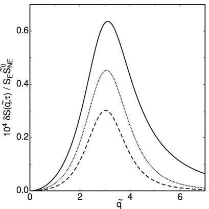
Figure 1: Difference ${\delta S(\tilde{q},\tau)}/{S_{\mathrm{E}}\tilde{S}^{0}_{\mathrm{NE}}}$ (see Eq. 16 below) between the theoretical structure factors at $R=1371$ (Eq. (14)), and at $R=0$ (Eq. (15)) as a function of $\tilde{q}$, for three different collecting times. The solid curve corresponds to $\tau=0$ ms, the dashed curve to $\tau=200$ ms, and the dotted curve to $\tau=500$ ms. The Prandtl number is $\sigma=34$ and $t_{\mathrm{v}}=0.74$ s.

In principle, $S(q,\tau)$ can be evaluated by substituting Eq. (3) with Eq. (4) for the correlation function of the density fluctuations into the right-hand side of Eq. (13). However, for the experimental results to be presented, it is sufficient to evaluate $S(q,\tau)$ for large values of the Prandtl number $\sigma$, in which case the exponential contribution with decay rate $\Gamma_{+}(q)$ in Eq. (4) can be neglected, as discussed before. Retaining only the contribution from the slower mode with amplitude $\tilde{A}_{-}(q)$ in Eq. (4) and performing the integrations, we deduce from Eq. (13)

$$S(\tilde{q},\tilde{\tau})=S_{\mathrm{E}}\tilde{A}_{-}(\tilde{q})\frac{\tilde{\tau}~{}\tilde{\Gamma}_{-}(\tilde{q})-1+\exp[-\tilde{\tau}~{}\tilde{\Gamma}_{-}(\tilde{q})]}{18\tilde{\tau}^{2}~{}\tilde{\Gamma}^{2}_{-}(\tilde{q})},$$ (14)

where $\tilde{\tau}$ is a dimensionless exposure time, defined by $\tilde{\tau}=\tau/t_{\mathrm{v}}$ with $t_{\mathrm{v}}$ the vertical relaxation time introduced in Eq. (5). In the limit $\tau\to 0$, Eq. (14) reduces to $S(\tilde{q})=S_{\mathrm{E}}\tilde{A}_{-}(\tilde{q})/36$, so that it equals the static structure factor measured in small-angle light-scattering or in shadowgraph experiments in the zero collecting time approximation, as given by Eq. (9). It is interesting to note that, due to the nonzero collecting time, $\tau$, even in thermal equilibrium ($R=0$) the shadowgraph measurements present some “structure”. From Eq. (14), we find that this equilibrium structure, as a function of the dimensionless collecting time, $\tilde{\tau}$, is given by

$$S_{\mathrm{E}}(\tilde{q},\tilde{\tau})=S_{\mathrm{E}}\frac{5}{3\tilde{\tau}^{2}}\frac{\tilde{\tau}(\tilde{q}^{2}+10)-1+\exp[-\tilde{\tau}(\tilde{q}^{2}+10)]}{(\tilde{q}^{2}+10)^{2}}.$$ (15)

It can be readily checked that, in the limit $\tau\to 0$, Eq. (15) reduces to the structureless constant $(5/6)S_{\mathrm{E}}$, in agreement with Eq. (9). This value is 17% lower than the actual value $S_{\mathrm{E}}$, due to the use of a first-order Galerkin approximation miPRE .

To gain insight into the effect of the exposure time on shadowgraph measurements, we show in Fig. 1 the difference between the nonequilibrium structure factor as obtained from Eq. (14) and the equilibrium structure factor ($R=0$) as obtained from Eq. (15), as a function of $\tilde{q}$, for three different collecting times. Corresponding to some of the experimental results to be discussed below, we used $R=1371$, a vertical relaxation time $t_{\mathrm{v}}=d^{2}/D_{T}$ of 0.74 s, and a Prandtl number $\sigma$ equal to 34. We evaluated the difference for $\tau=0$, $\tau=200$, and $\tau=500$ ms. The structure factors $S(q,\tau)$ and $S_{\mathrm{E}}(q,\tau)$ have been normalized by dividing them by the product $S_{\mathrm{E}}\tilde{S}_{\mathrm{NE}}^{0}$.

From Fig. 1, we arrive at the following conclusions: (i) The main effect of a nonzero collecting time is to lower the height of the measured $S(q,\tau)$; this is expected since fluctuations cancel out when larger exposure times are used. (ii) An additional effect of a nonzero collecting time, which can be observed in Fig. 1, is a displacement of the maximum in $S(q,\tau)$ to lower $\tilde{q}$ values. This effect is mainly due to the subtraction of the equilibrium structure given by Eq. (15), which decreases with increasing $\tilde{q}$. (iii) Another interesting feature, we infer from Fig. 1, is that the dependence on $\tilde{q}^{2}$ for low $\tilde{q}$ is preserved, while the dependence on $\tilde{q}^{-4}$ for large $\tilde{q}$ is destroyed for the effective structure factor. Actually, at large $q$, there exists a crossover from a $q^{-4}$ dependence to a $q^{-6}$ dependence, for nonzero values of $\tau$, as will be shown below in Eq. (17).

A simpler formula for $S(\tilde{q},\tilde{\tau})$ can be obtained by introducing into Eq. (14) the limiting value of $\tilde{A}_{-}(q)$ for large Prandtl numbers. We then obtain

$$\frac{\delta S(\tilde{q},\tau)}{S_{\mathrm{E}}\tilde{S}^{0}_{\mathrm{NE}}}=\frac{S(\tilde{q},\tilde{\tau})-S_{\mathrm{E}}(\tilde{q},\tilde{\tau})}{S_{\mathrm{E}}\tilde{S}^{0}_{\mathrm{NE}}}\\ =\frac{5}{3\sigma}\frac{\tilde{\tau}\tilde{\Gamma}_{-}(\tilde{q})-1+\exp[-\tilde{\tau}\tilde{\Gamma}_{-}(\tilde{q})]}{\tau^{2}~{}\tilde{\Gamma}^{2}_{-}(\tilde{q})}\\ \hfill\times\frac{27\tilde{q}^{2}}{28(\tilde{q}^{2}+10)(\tilde{q}^{4}+24\tilde{q}^{2}+504)-27R\tilde{q}^{2}},$$ (16)

where for $\tilde{\Gamma}_{-}(\tilde{q})$ Eq. (8) for large $\sigma$ should be used. As discussed after Eq. (8), for Prandtl numbers near 15 the asymptotic limit (16) is already closely approached. Equation (16) reduces, in the limit $\tau\to 0$, to the expressions obtained in Ref. miPRE . It is interesting to note that, in the limit $\tilde{q}\to\infty$, Eq. (16) reduces to:

$$\frac{\delta S(\tilde{q},\tau)}{S_{\mathrm{E}}\tilde{S}^{0}_{\mathrm{NE}}}\xrightarrow{\tilde{q}\to\infty}~{}\frac{45}{28\tilde{\tau}\sigma}~{}\frac{1}{\tilde{q}^{6}},$$ (17)

showing, as mentioned above, that a nonzero collecting time changes the asymptotic behavior from $q^{-4}$ to $q^{-6}$. Note that Eq. (17) is evidently not valid when $\tau=0$ in which case one needs the asymptotic expression given by Eq. (30) in Ref. miPRE .

IV Experiments

IV.1 Apparatus

To visualize the thermal fluctuations with the shadowgraph method one needs to perform the experiments with a fluid in which the thermal noise will be large HohenbergSwift ; VanBeijerenCohen . This goal can be accomplished by selecting a fluid in the vicinity of its critical point WuEtAl ; DeBruynEtAl ; OA03 . The measurements reported here were obtained for sulfur hexafluoride. The apparatus and experimental procedures have been described in detail elsewhere DeBruynEtAl . Here we describe only those aspects which are specific to the experiment with a fluid near its critical point.

For the details of the cell construction we refer to Fig. 9 of Ref. DeBruynEtAl . Initially we used a diamond-machined aluminum bottom plate which could be positioned with piezo-electric elements. The bottom-plate thermistors were embedded approximately 0.64 cm below its top surface. Even though to the naked eye this plate had a near-perfect mirror finish, the tool marks from the diamond machining imposed a preferred direction on the fluctuations below the onset of convection. Thus we placed an optically flat sapphire of thickness 0.318 cm on top of the aluminum plate. A thin silver film was evaporated on the top surface of this sapphire to provide a mirror for the shadowgraphy.

Initially we used a sapphire of thickness 0.952 cm for the cell top. In addition a sapphire of thickness 1.90 cm was in the optical path of the shadowgraphy and provided the top window of the pressure vessel. In combination with the very small cell thickness used in these experiments, it turned out that the optical anisotropy of these randomly oriented sapphires introduced an anisotropy of the shadowgraph images which obscured the rotational symmetry of the fluctuations. In order to minimize this effect, we replaced the pressure window by a fused-quartz window and used an optically flat sapphire of 0.318 cm thickness for the cell top. Under these conditions we found that the fluctuations below the onset of convection yielded a structure factor which was nearly invariant under rotation, as can be seen from Fig. 5 below.

The cell spacing was fixed by a porous paper sidewall with an inner (outer) diameter of 2.5 (3.5) cm. Since the top sapphire was supported along its perimeter which had a diameter of 10 cm (i.e., considerably larger than the cell wall), the force exerted on the cell top by the bottom plate and the wall caused a slight bowing of the initially flat top. Over the entire sample diameter this yielded a radial cell-spacing variation corresponding to about one circular fringe when illuminated with an expanded parallel He-Ne laser beam. This variation of the thickness by about 0.3 $\mu$m assured that convection would start in the cell center, rather than being nucleated inhomogeneously near the cell wall. Assuming a parabolic radial profile for the cell spacing, we estimate that the spacing was uniform to much better than 0.1% over the 1.3$\times$1.3 cm² area near the cell center which was actually used for the shadowgraph images. The actual sample thickness was measured interferometrically DeBruynEtAl and found to be 34.3 $\mu$m.

IV.2 Properties of SF₆ near the critical point

The thermodynamic properties of sulfur hexafluoride in the critical region can be calculated from a equation developed by Wyczalkowska and Sengers WS99 . For the viscosity we used a fit of data from Refs. HBT85 and SV89 to a smooth function. This approach neglects a small anomaly of the viscosity at the critical point. We used fits of smooth functions to the conductivity data from Refs. LK65 ; SH73 ; LimSwinney ; Li73 ; BT81 ; KI85 .

The measurements were made at constant pressure $P$ and at constant mean sample temperature $\bar{T}$. The mean temperature was adjusted so that the density $\rho(\bar{T})$ was the critical density $\rho_{\mathrm{c}}=742$ kg m^-3. The imposed temperature difference $\Delta T$ caused a density variation of the sample along an isobar. This is illustrated in Fig. 2 for the conditions of the present experiments, namely for $P=38.325$ bar and $\bar{T}=46.50^{\circ}$C. At $\rho=\rho_{\mathrm{c}}$, we have $\sigma=34.0$, $D_{T}=1.59\times 10^{-5}$ cm²/s, and $t_{\mathrm{v}}\equiv d^{2}/D_{T}=0.738$ s.

Figure 2: The temperature-density plane near the critical point of SF₆. The dashed line indicates the coexistence curve separating liquid and vapor. The vertical dotted line is the critical isochore. The solid circle is the critical point with $T_{\mathrm{c}}=45.567^{\circ}$C, $P_{\mathrm{c}}=37.545$ bar, $\rho_{\mathrm{c}}=0.742$ g/cm³. The solid line represents the isobar $P=38.325$ bar used in our measurements, and the heavy section of this line shows the temperature-density range on the isobar which is spanned by the sample with thickness $d=34.3~{}\mu$m when $\Delta T=0.22^{\circ}$C.

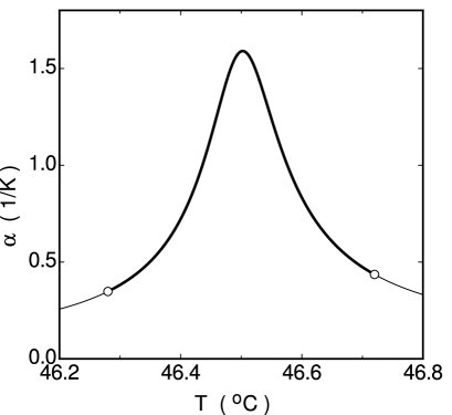
Figure 3: The thermal expansion coefficient $\alpha$ along the isobar $P=38.325$ bars. The heavy part of the line terminated by two open circles indicates the temperature range spanned by the sample with $d=34.3~{}\mu$m and $\Delta T=\Delta T_{\mathrm{c}}=0.44^{\circ}$C.

IV.3 Symmetric departures from the Oberbeck-Boussinesq approximation

Much of the theoretical work on RBC has been done in the OB approximation Bo03 ; Ob79 , which assumes that the fluid properties do not vary over the imposed temperature interval, except for the density where it provides the buoyant force Ch61 . Non-OB effects have been considered by a number of investigators, and most systematically by Busse Bu67a . At leading order, they break the reflection symmetry of the system about the horizontal midplane, and at the onset of convection they yield a transcritical bifurcation to a hexagonal pattern BPA00 , instead of the roll pattern of pure OB convection. When the mean temperature corresponds to the critical isochore, $\rho=\rho_{\mathrm{c}}$, this effect is of modest size. Although several properties contribute, we illustrate this by showing the isobaric thermal expansion coefficient in Fig. 3 along the isobar of Fig. 2 as an example. One can approximate $\alpha$ as a sum of two contributions, one of which is anti-symmetric and the other one symmetric about the mean temperature (and thus approximately also about the horizontal midplane) of the sample. Only the anti-symmetric part is considered in the theory Bu67a . Its smallness near the onset of convection is seen from the similar values of $\alpha$ at the top and bottom of the cell (open circles in the figure). A quantitative calculation of the parameter $\cal P$ introduced by Busse Bu67a (see Eqs. (13) in Ref. BPA00 ) yields ${\cal P}=-0.23$. This value indicates that, within our experimental resolution, only rolls should be seen near onset. This is indeed the case OA03 . However, the variation of $\alpha$ which is symmetric about the midplane is quite large. It does not break the reflection symmetry about that plane and thus permits the existence of rolls at onset rather than requiring a hexagonal plan form. Behavior similar to that of $\alpha$ is found for the specific heat $c_{P}$ and for the Rayleigh number. At present there is no theoretical treatment of these higher-order non-OB effects. Thus we proceed empirically by examining the variation of $R$ as a function of vertical position or local sample temperature. If we neglect the temperature dependence of the thermal conductivity and assume that the local temperature in the fluid layer still varies linearly as a function of $z$, we obtain the Rayleigh number profiles shown in Fig. 5. The curve at the top is for the experimental value $\Delta T=\Delta T_{\mathrm{c}}=0.44^{\circ}$C corresponding to the onset of convection. The other curves, from top to bottom, correspond to $\Delta T/\Delta T_{\mathrm{c}}=$0.860, 0.699, 0.430, and 0.269. For $\Delta T=0.44^{\circ}$C one sees that the local $R(\rho_{\mathrm{c}})\simeq 3190$ far exceeds the value $R_{\mathrm{c}}=1708$ for the uniform system. On the other hand, near the top and bottom of the sample the local $R$ is well below the onset of convection for the homogeneous system. The data in Fig. 5 show that, though we find rolls above threshold, non-OB effects cannot be completely neglected in our experiments. We shall return to the influence of non-OB effects on the comparison between experiment and theory in Sect. V.

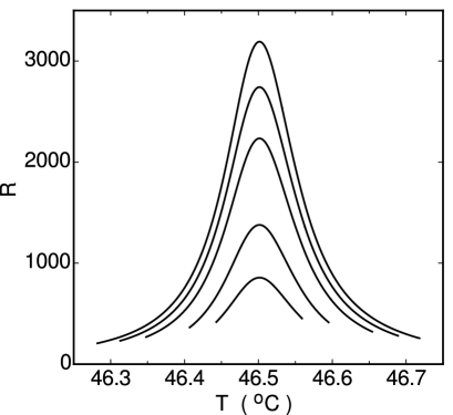
Figure 4: The Rayleigh number $R$ (see Eq. (1)) along the isobar $P=38.325$ bar for $d=34.3~{}\mu$m. From top to bottom, the curves are for $\Delta T/\Delta T_{\mathrm{c}}=1.000$, 0.860, 0.699, 0.430, and 0.269 with $\Delta T_{\mathrm{c}}=0.44^{\circ}$C.

IV.4 Sample temperature

The bath temperature $T_{\mathrm{bath}}$ and the bottom-plate temperature $T_{\mathrm{BP}}$ were adjusted so as to hold the mean sample temperature constant. This temperature was chosen so that the mean density corresponded to the critical density $\rho_{\mathrm{c}}$. Because of the small sample thickness the thermal resistance of the sample was comparable to that of the top and bottom confining plates. This fact required a special procedure to assure that the sample was indeed at the temperature corresponding to $\rho_{\mathrm{c}}$. Before a run at a given fixed pressure was started, we measured the power of shadowgraph images of the fluctuations at a fixed imposed $\Delta T_{\mathrm{ext}}=(T_{\mathrm{BP}}-T_{\mathrm{bath}})$ as a function of the mean temperature $\bar{T}_{\mathrm{ext}}=(T_{\mathrm{BP}}+T_{\mathrm{bath}})/2$ of the system consisting of the bottom plates, the sample, and the top plate as determined by the bath temperature and the bottom-plate thermistor. This temperature difference is the sum of those across the bottom aluminum plate $\Delta T_{\mathrm{Al}}$, across the boundary between the aluminum plate and the bottom sapphire $\Delta T_{\mathrm{b1}}$, across the bottom sapphire $\Delta T_{\mathrm{sb}}$, across the sample $\Delta T$, across the top sapphire $\Delta T_{st}$, and across a boundary layer above the top sapphire in the water bath $\Delta T_{\mathrm{b2}}$. From estimates of the thermal resistances of these sections we find $\Delta T/\Delta T_{\mathrm{ext}}=0.473$. Thus, at the onset of convection, we measured $\Delta T_{\mathrm{ext,c}}=0.930^{\circ}$C and deduced $\Delta T_{\mathrm{c}}=0.44^{\circ}$C.

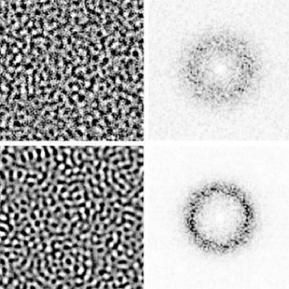
Figure 5: Shadowgraph signals (left column) and the moduli squared of their Fourier transforms (right colum) for $\Delta T=0.189$ (top row) and $\Delta T=0.378$ K (bottom row). The exposure time was 500 ms.

IV.5 Analysis of shadowgraph images

At each $\Delta T$, three shadowgraph-image sequences $I_{i}({\bf x},\tau_{j}),~{}i=1,...,N$ with $N=1024$, and $j=0,1,2$ were acquired. For each sequence, a different exposure time $\tau_{j}$ was used, namely $\tau_{0}$ = 0.500 s, $\tau_{1}$ = 0.350 s, and $\tau_{2}$ = 0.200 s. The time interval $\delta t$ between the images was typically one or two seconds, which was large enough for the images to be nearly uncorrelated. The images of each sequence were averaged to provide a background image $I_{0}({\bf x},\tau_{j})$, as discussed in Sect. III. Then, for each image of the sequence, a dimensionless shadowgraph signal $\mathcal{I}_{i}({\bf x},\tau_{j})$ was computed, in accordance with Eq. (10). The mean (over $\bf x$) value of a typical ${\cal I}_{i}(\mathbf{x},\tau_{j})$ was within the range $\pm 0.01$, indicating adequate stability of the light intensity and image-acquisition system. Next, the two-dimensional Fourier transform of each shadowgraph signal in the sequence was computed, and the modulus square calculated, obtaining series of $|\mathcal{I}_{i}(\mathbf{q},\tau_{j})|^{2}$ for further analysis. Typical shadowgraph signals and the squares of the moduli of their Fourier transforms are shown in Fig. 5. The nearly-uniform angular distribution of the transforms illustrates the rotational invariance of the Rayleigh-Bénard system.

As explained in Sect. III, due to the rotational invariance of RB convection in the horizontal plane, the modulus squared Fourier transformed shadowgraph signals have rotational symmetry, and for an infinitely extended sample they would depend only on the modulus $q$ of the wave vector $\mathbf{q}$. However, the finite spatial extent of the images leads to random angular fluctuations of $|\mathcal{I}_{i}(\mathbf{q},\tau_{j})|^{2}$. To reduce these fluctuations, we performed azimuthal averages $\overline{|\mathcal{I}_{i}(\mathbf{q},\tau_{j})|^{2}}$ over thin rings in Fourier space (the angular average is denoted by the overline and depends only on $q$ and $\tau_{j}$). Now for each shadowgraph measurement $I_{i}(\mathbf{x},\tau_{j})$ the integral

$$P_{i}(\tau_{j})=\int_{0}^{\infty}2\pi q~{}\overline{|\mathcal{I}_{i}(\mathbf{q},\tau_{j})|^{2}}~{}dq$$ (18)

is the total power and, by Parseval’s theorem, has to be equal to the variance of the original $\mathcal{I}_{i}({\bf x},\tau_{j})$. We used Eq. (18) as a check of consistency for the entire procedure of taking the Fourier transform, of calculating the modulus squared and the azimuthal average over thin rings, and of assigning to each ring a $q$ value. Finally, we averaged over the $N$ individual $\overline{|\mathcal{I}_{i}(\mathbf{q},\tau_{j})|^{2}}$ of each $\tau_{j}$ series, to obtain the experimental shadowgraph structure factor $S_{\mathrm{s}}(q,\tau_{j})\equiv\langle\overline{|\mathcal{I}_{i}(\mathbf{q},\tau_{j})|^{2}}\rangle$.

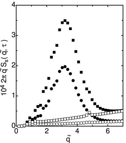
Figure 6: Experimental shadowgraph structure factor $2\pi\tilde{q}S_{\mathrm{s}}(\tilde{q},\tau)$ as a function of the dimensionless wave number $\tilde{q}$. These results are for $P=38.325$ bar, $\bar{T}=46.5^{\circ}$C, and $\Delta T=0.189^{\circ}$C. The solid squares (solid circles) are for $\tau=0.200$ s ($\tau=0.500$ s). The open symbols are the corresponding background measurements for $\Delta T=0$.

For the remainder of this paper we shall use the experimentally determined cell spacing $d=34.3\mu$m to scale $q$ according to $\tilde{q}=qd$. Two examples of the product $2\pi\tilde{q}S_{\mathrm{s}}(\tilde{q},\tau_{j})$, both for $P=38.325$ bar, $\bar{T}=46.5^{\circ}$C, and $\Delta T=0.189^{\circ}$C, are shown in Fig. 6. The solid squares are for $\tau_{2}=0.200$ s, whereas the solid circles are for $\tau_{0}=0.500$ s. As discussed in the previous section, the relationship (12) between the experimental shadowgraph structure factor $S_{\mathrm{s}}(\tilde{q},\tau_{j})$ and the corresponding fluid structure factor $S(\tilde{q},\tau_{j})$ involves the optical transfer function $\mathcal{T}(\tilde{q})$. Nevertheless, we observe some qualitative agreement of the experimental results for $2\pi\tilde{q}S_{\mathrm{s}}(\tilde{q},\tau)$ in Fig. 6 and the theoretical results for $S(\tilde{q},\tau)$ shown in Fig. 1. The expected maximum near $\tilde{q}=\tilde{q}_{c}$ is present, and the decrease as $\tilde{q}$ vanishes is consistent with the predicted $\tilde{q}^{2}$ dependence. The longer averaging of the random fluctuations diminishes $2\pi\tilde{q}~{}S_{\mathrm{s}}(\tilde{q},\tau)$, which was one of the features noted after Fig. 1 for $S(\tilde{q},\tau)$.

The experimental structure factor $S_{\mathrm{s}}(\tilde{q},\tau_{j},\Delta T)$ depends on the Rayleigh number and, hence, on $\Delta T$. For $\Delta T=0$, instrumental (mostly camera) noise is expected to be the dominant contribution, i.e., the contribution from the equilibrium fluctuations is negligible and the theoretical equilibrium structure, given by Eq. (15), is expected to be unobservable in our experiments. Examples of the shadowgraph structure factors for $\Delta T=0$ are shown by the open symbols in Fig. 6. One sees that $2\pi\tilde{q}S_{s}(\tilde{q},\tau_{j},0)$ is well represented by a straight line, corresponding to white noise. At large $\tilde{q}$, $2\pi\tilde{q}S_{s}(\tilde{q},\tau_{j},0)$ merges smoothly into the data for the $2\pi\tilde{q}S_{s}(\tilde{q},\tau_{j},\Delta T)$ with the same $\tau_{j}$, as one would expect.

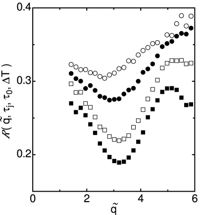
Figure 7: The ratio ${\cal R}(\tilde{q},\tau_{j},\tau_{0},\Delta T)$ (see Eq. (20)) based on $\tau_{j}=0.200$ s and $\tau_{0}=0.500$ s. From top to bottom the data are for $\Delta T=0.118,~{}0.189,~{}0.307$ and $0.378^{\circ}$C. The onset of convection occurred at $\Delta T_{\mathrm{c}}=0.440^{\circ}$C.

A detailed comparison between the experimental and the theoretical structure factors requires knowledge of the optical transfer function, $\mathcal{T}(\tilde{q})$, which depends on the details of the experimental optical arrangement. It involves, for instance, the size of the pinhole and the focal length of the lens used to make the “parallel” beam, and the spectral width of the light source.TC02 In the present work the spatial structures to be determined (the fluctuation wavelengths) had length scales [typically ${\cal O}(50~{}\mu{\rm m})$] that are one or two orders of magnitude smaller than those of more conventional RB experiments. For this reason, we found it difficult to obtain ${\cal T}(\tilde{q})$ for our instrument with sufficient accuracy to avoid significant distortion of $S(\tilde{q})$. We circumvented the difficulty of the optical transfer function by deriving the dynamic properties of the fluctuations from ratios of $S_{\mathrm{s}}(\tilde{q},\tau_{j})$ with different values of $\tau_{j}$. To account for the instrumental white noise, before taking such ratios, we subtracted the measured $S_{\mathrm{s}}(\tilde{q},\tau_{j},0)$ in the absence of a temperature gradient from $S_{\mathrm{s}}(\tilde{q},\tau_{j},\Delta T)$ to yield

$$\delta S_{\mathrm{s}}(\tilde{q},\tau_{j},\Delta T)=S_{s}(\tilde{q},\tau_{j},\Delta T)-S_{\mathrm{s}}(\tilde{q},\tau_{j},0).$$ (19)

After this background subtraction, we formed for $j=1,2$ the ratio

$${\cal R}(\tilde{q},\tau_{j},\tau_{0},\Delta T)\equiv\frac{\tau_{j}^{2}~{}\delta S_{\mathrm{s}}(\tilde{q},\tau_{j},\Delta T)}{\tau_{0}^{2}~{}\delta S_{\mathrm{s}}(\tilde{q},\tau_{0},\Delta T)}\ .$$ (20)

where $\tau_{0}$ is the longest exposure time $\tau_{0}=0.500$ s. The ratios $\mathcal{R}$ obtained for $\tau_{j}=0.200$ s as a function of $\tilde{q}$ are shown in Fig. 7 for four values of the temperature difference $\Delta T$. The shadowgraph transfer function ${\cal T}(\tilde{q})$ cancels and is no longer contained in ${\cal R}$. In addition, for the ratios $\mathcal{R}$, it is irrelevant whether we use the definition of the structure factor considered in Sect. II, or the shadowgraph definition displayed in Fig. 6, the latter including a factor $2\pi\tilde{q}$. Thus, we are allowed to use Eq. (14) for $\delta S_{\mathrm{s}}$, so that

$${\cal R}(\tilde{q},\tau_{j},\tau_{0},\Delta T)=\frac{\tau_{j}\Gamma(\tilde{q})-1+\exp(-\tau_{j}\Gamma(\tilde{q}))}{\tau_{0}\Gamma(\tilde{q})-1+\exp(-\tau_{0}\Gamma(\tilde{q}))}\ .$$ (21)

One sees that ${\cal R}$ depends only on $\tau_{0},\tau_{j},\tilde{q},$ and $\Gamma(\tilde{q},\Delta T)$. At each $\tilde{q}$ and $\Delta T$, only the decay rate $\Gamma$ is unknown and thus can be determined from the experimental value of $\cal R$.

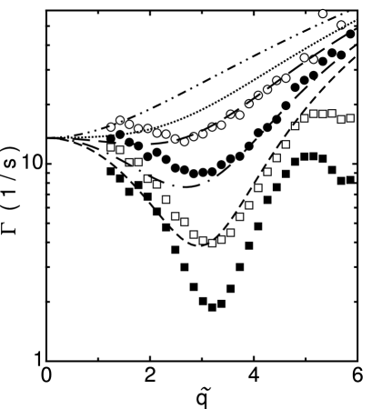
Figure 8: Results for $\Gamma(\tilde{q},\Delta T)$, in units of inverse seconds, obtained from the values of $\cal R$ shown in Fig. 7 (see Eq. (21)). The symbols are the same as in Fig. 7. The top (dash-double-dotted) curve is the prediction for $\Delta T=0$. The remaining curves are the theoretical predictions (see Eq. (8)) for the values of $\Delta T$ of the data (see Fig. 7).

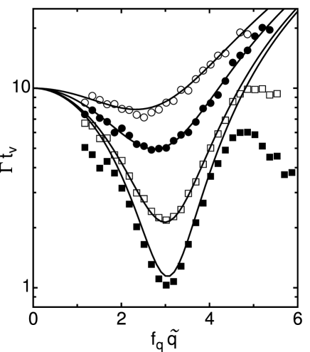
Figure 9: Results for $\Gamma t_{\mathrm{v}}$ as a function of $f_{q}\tilde{q}$, using the values $t_{\mathrm{v}}=0.551$ s and $f_{q}=0.944$ from the least-squares fit described in the text. The data and symbols correspond to those in Fig. 8. The curves indicate the corresponding theoretical results obtained from Eq. (8) by using the scale factors of the Rayleigh number $f_{R,k}$ from the least-squares fit.

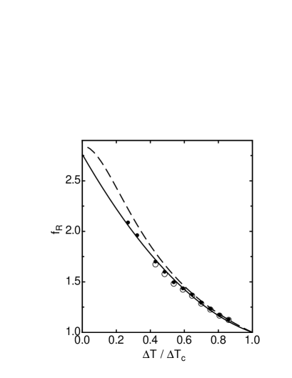
Figure 10: Values of the fit parameter $f_{R,k}$ obtained from the least-squares fit described in the text. Solid symbols correspond to $\Gamma$ based on exposure times $\tau_{0}=0.500$ s and $\tau_{j}=0.200$ s. For the open symbols $\tau_{j}$ was 0.350 s. The solid curve is the polynomial $f_{R}=2.74-2.87\Delta T/\Delta T_{\mathrm{c}}+1.13(\Delta T/\Delta T_{\mathrm{c}})^{2}$ which passes through the point (1,1). The dashed curve represents $\langle R\rangle/\langle R\rangle_{\mathrm{c}}$ and was calculated from values of $R$ like those shown in Fig. 5.

V Experimental results and comparison with theory

In Fig. 8 we show the decay rate $\Gamma$ as a function of $\tilde{q}$. The symbols represent the experimental values deduced from the data for $\mathcal{R}$ displayed in Fig. 7 by solving Eq. (21). From top to bottom, the data sets are for $\Delta T/\Delta T_{\mathrm{c}}=$ 0.269, 0.430, 0.698, and 0.861. The curves represent the theoretical values calculated from Eq. (8) with $t_{\mathrm{v}}=0.738$ s (the value derived from the fluid properties at the mean temperature and at the critical density). The topmost (dash-double-dotted) line is for equilibrium: $\Delta T=0$ (i.e., $R=0$). The remaining four curves are for the values of $\Delta T/\Delta T_{\mathrm{c}}$ of the data sets, if we adopt the Boussinesq estimate

$$R_{\mathrm{OB}}=(\Delta T/\Delta T_{\mathrm{c}})R_{\mathrm{c}}$$ (22)

with $R_{\mathrm{c}}=1730$ (the value obtained from the Galerkin approximation used in this paper Manneville ) for the Rayleigh number in Eq. (2). One sees that the predictions, based on the Boussinesq approximation, do not agree very well with the experiment. However, both theory and experiment reveal clearly a minimum of $\Gamma$ near $\tilde{q}\simeq 3$ which becomes more pronounced as $\Delta T$ approaches $\Delta T_{\mathrm{c}}$. For the larger values of $\Delta T/\Delta T_{\mathrm{c}}$ the experimental values of $\Gamma$ have a maximum near $\tilde{q}=5$. We expect that this is due to nonlinear effects in the physical system which lead to second-harmonic generation. This phenomenon is not contained in the theory.

We believe that the major disagreement between the measurements and the calculation is due to symmetric non-OB effects discussed in Sect. IV.3. Since there is no quantitative theory, we proceeded empirically and explored the possibility that non-OB effects can be accommodated to a large extent by multiplying the experimental $\Delta T/\Delta T_{\mathrm{c}}$ used to estimate $R$ by an adjustable scale factor. We introduced an adjustable parameter $f_{R,k}$ which was allowed to be different for each $\Delta T_{k}$ and used

$$R_{k}=f_{R,k}R_{\mathrm{OB}}$$ (23)

for the Rayleigh number. In addition, we introduced a single adjustable scale factor for all data sets which adjusted the length scale of the experiment so as to yield a corrected wave number

$$\tilde{q}_{\mathrm{corr}}=f_{q}\tilde{q}.$$ (24)

to be used in the fit of the theory to the data. We expect $f_{q}$ to compensate for experimental errors in the cell spacing and in the spacing between the pixels of the images, to be within a few percent of unity, and to be the same for the runs at all $\Delta T$. Finally, we treated the vertical relaxation time $t_{\mathrm{v}}$ as an adjustable parameter. We note that $t_{\mathrm{v}}=d^{2}/D_{T}$ depends on the cell spacing, and thus any error in the length scale will lead to an error in the time scale $t_{\mathrm{v}}$. One also might expect $t_{\mathrm{v}}$ to depend on $\Delta T$ because quadratic non-OB effects would be larger at larger $\Delta T$; but it turned out that a single value for $t_{\mathrm{v}}$ for the runs at all $\Delta T$ was sufficient to describe all the data. We carried out a simultaneous least-squares fit of Eq. (21) to a group of 11 data sets of $\Gamma$, like those in Fig. 8, based on $\tau_{0}=0.500$ s and $\tau_{j}=0.200$ s. Each data set was for a different $\Delta T_{k}$, and collectively they spanned the range $0.27\leq\Delta T_{k}/\Delta T_{\mathrm{c}}\leq 0.86$. A separate fit was done to the second group of 9 available data sets based on $\tau_{0}$ = 0.500 s and $\tau_{j}=0.350$ s. For each group we simultaneously adjusted $f_{q},t_{\mathrm{v}}$, and the eleven or nine $f_{R,k}$. We obtained the same result $f_{q}=0.944\pm 0.010$ from both groups. The fit also gave $t_{\mathrm{v}}=0.551\pm 0.02$ ($0.565\pm 0.029$) s for the group based on $\tau_{j}=0.200~{}(0.350)$ s. Qualitatively consistent with the expected influence of the symmetric non-OB effects, the fitted value of $t_{\mathrm{v}}$ is somewhat smaller than the value 0.738 s estimated for $\rho=\rho_{\mathrm{c}}$ and the experimental value $d=34.3~{}\mu$m. As said above, part of this difference is attributable to the error in $d$ indicated by the result obtained for $f_{q}$. In Fig. 9 we show the results for the product $\tilde{\Gamma}=\Gamma t_{v}$ for the four examples displayed in Fig. 8 as a function of $f_{q}\tilde{q}$, together with the corresponding predictions generated by using the values of $f_{R,k}$ from the fit. Except for the second-harmonic contribution at large $\tilde{q}$ and $\Delta T$, the adjusted theory agrees quite well with the data.

The values obtained for $f_{R,k}$ are given in Fig. 10. The two groups ($\tau_{j}=0.200$ s and $\tau_{j}=0.350$ s) agree very well with each other, showing that consistent results are obtained with different exposure times. Also shown is a fit to the data sets with $\tau_{j}=0.200$ s in which the individual $f_{R,k}$ were replaced by a quadratic function which was forced to pass through $f_{R,k}=1$ at $\Delta T=\Delta T_{\mathrm{c}}$. This fit gave

$$f_{R}(\Delta T/\Delta T_{\mathrm{c}})=2.74-2.87\frac{\Delta T}{\Delta T_{\mathrm{c}}}+1.13\left(\frac{\Delta T}{\Delta T_{\mathrm{c}}}\right)^{2}\ .$$ (25)

This two-parameter representation of $f_{R}$ fits the data equally well.

One sees that $f_{R}$ is largest at the smallest $\Delta T$, indicating that the estimate $R=R_{\mathrm{OB}}$ (see Eq. (22)) becomes worse as $\Delta T$ decreases. This is to be expected because the approximation for $f_{R}$ must approach unity as $\Delta T$ approaches $\Delta T_{\mathrm{c}}$ in order for $\Gamma(\tilde{q}_{\mathrm{c}},\Delta T_{\mathrm{c}})$ to vanish. As a simplest empirical attempt to include non-OB effects in the comparison between experiment and theory, we define, in analogy to Eq. (22), a non-Boussinesq Rayleigh number

$$R_{\mathrm{NOB}}(\Delta T)=\frac{\langle R(\rho)\rangle}{\langle R(\rho)\rangle_{\mathrm{c}}}~{}R_{\mathrm{c}},$$ (26)

where as before $R_{\mathrm{c}}=1730$ and where the angular bracket indicates an average over the spanned temperature (and thus density) range along the isobar. The averaged critical Rayleigh number $\langle R(\rho)\rangle_{\mathrm{c}}$ is equal to $\langle R(\rho)\rangle$ for $\Delta T=\Delta T_{\mathrm{c}}$. It turns out that $\langle R(\rho)\rangle_{\mathrm{c}}=1120$ for our experiment. This approximation corresponds to a re-defined

$$f_{R}(\Delta T)=\frac{\Delta T_{\mathrm{c}}}{\Delta T}~{}\frac{\langle R(\rho)\rangle}{\langle R(\rho)\rangle_{\mathrm{c}}}\ .$$ (27)

We note that by definition $f_{R}(\Delta T_{\mathrm{c}})=1$ and thus $R=1730$ as it should be. Equation (27) is plotted in Fig. (10) as a dashed line. One sees that this simplest non-OB model accounts very well for the experimental data of $f_{R}$. Of course, it would be very helpful to have a proper theory (rather than an empirical model) of this interesting effect.

VI Summary

In this paper we have reported on experimental and theoretical studies of the dynamics of thermal fluctuations below the onset of Rayleigh-Bénard convection in a thin horizontal fluid layer bounded by two rigid walls and heated from below. Starting from the fluctuating linearized Boussinesq equations, we derived theoretical expressions for the dynamic structure factor and the decay rates and amplitudes of the hydrodynamic modes that characterize the dynamics of the fluctuations. The dynamic structure factor is dominated by a slow mode with a decay rate that vanishes as the Rayleigh number $R$ becomes equal to its critical value $R_{\mathrm{c}}$ for the onset of convection.

We used the shadowgraph method to determine the ratio $\cal R$ of shadowgraph structure factors obtained with different camera exposure times. From the theoretical results for the dynamic structure factor, we derived a relationship between this ratio and the decay rates of the fluctuations. Using this result and the experimental values of $\cal R$, we obtained experimental decay-rate data for a wide range of temperature gradients below the onset of Rayleigh-Bénard convection in sulfur hexafluoride near its critical point. Quantitative agreement between the experimental decay rates and the theoretical prediction could be obtained when allowance was made for some experimental uncertainty in the small spacing between the plates and an empirical estimate was employed for symmetric deviations from the Oberbeck-Boussinesq approximation which are expected in a fluid with its mean density on the critical isochore.

VII ACKNOWLEDGEMENTS

The research of J. Oh and G. Ahlers was supported by U.S. National Science Foundation Grant DMR02-43336. G. Ahlers and J. M. Ortiz de Zárate acknowledge support through a Grant under the Del Amo Joint Program of the University of California and the Universidad Complutense de Madrid. The research at the University of Maryland was supported by the Chemical Sciences, Geosciences and Biosciences Division of the Office of Basic Energy of the U.S. Department of Energy under Grant No. DE-FG-02-95ER14509.

References

- (1) T. R. Kirkpatrick, E. G. D. Cohen, and J. R. Dorfman, Phys. Rev. A 26, 995 (1982).
- (2) B. M. Law and J. V. Sengers, J. Stat. Phys. 57, 531 (1989).
- (3) P. N. Segrè, R. W. Gammon, J. V. Sengers, and B. M. Law, Phys. Rev. A 45, 714 (1992).
- (4) J. M. Ortiz de Zárate and J. V. Sengers, Phys. Rev. E 66, 036305 (2002).
- (5) P. N. Segrè, R. Schmitz, and J. V. Sengers, Physica A 195, 31 (1993).
- (6) A. Vailati and M. Giglio, Phys. Rev. Lett. 77, 1484 (1996).
- (7) J. M. Ortiz de Zárate, R. Pérez Cordón, and J. V. Sengers, Physica A 291, 113 (2001).
- (8) J. M. Ortiz de Zárate and J. V. Sengers, Physica A 300, 25 (2001).
- (9) V. Zaitsev and M. Shliomis, Sov. Phys. JETP 32, 866 (1971).
- (10) J. B. Swift and P. C. Hohenberg, Phys. Rev. A 15, 319 (1977).
- (11) P. C. Hohenberg and J. B. Swift, Phys. Rev. A 46, 4773 (1992).
- (12) M. Wu, G. Ahlers, and D. S. Cannell, Phys. Rev. Lett. 75, 1743 (1995).
- (13) J. Oh and G. Ahlers, Phys. Rev. Lett. 91, 094501 (2003).
- (14) B. M. Law, P. N. Segrè, R. W. Gammon, and J. V. Sengers, Phys. Rev. A 41, 816 (1990).
- (15) H. N. W. Lekkerkerker and J. P. Boon, Phys. Rev. A 10, 1355 (1974).
- (16) J. P. Boon, C. Allain, and P. Lallemand, Phys. Rev. Lett. 43, 199 (1979).
- (17) P. Lallemand and C. Allain, J. Phys. (Paris) 41, 1 (1980).
- (18) R. Schmitz and E. G. D. Cohen, J. Stat. Phys. 40, 431 (1985).
- (19) T. R. Kirkpatrick and E. G. D. Cohen, J. Stat. Phys. 33, 639 (1983).
- (20) C. Allain, H. Z. Cummins, and P. Lallemand, J. Phys. (Paris) Lett. 39, L473 (1978).
- (21) Y. Sawada, Phys. Lett. A 65, 5 (1978).
- (22) A. M. Pedersen and T. Riste, Z. Phys. B 37, 171 (1980).
- (23) K. Otnes and T. Riste, Phys. Rev. Lett. 37, 1490 (1980).
- (24) R. Behringer and G. Ahlers, Phys. Lett. 62A, 329 (1977).
- (25) J. Wesfreid, Y. Pomeau, M. Dubois, C. Normand, and P. Bergé, J. Phys. (France) 39, 725 (1978).
- (26) A. Oberbeck, Ann. Phys. Chem. 7, 271 (1879).
- (27) J. Boussinesq, Théorie Analytique de la Chaleur (Gauthier-Villars, Paris, 1903), Vol. 2.
- (28) S. Chandrasekhar, Hydrodynamic and Hydromagnetic Stability (Oxford University Press, Oxford, 1961).
- (29) J. K. Platten and J. C. Legros, Convection in Liquids (Springer, Berlin, 1984).
- (30) P. Manneville, Dissipative Structures and Weak Turbulence (Academic Press, San Diego, 1990).
- (31) M. C. Cross and P. C. Hohenberg, Rev. Mod. Phys. 65, 851 (1993).
- (32) L. D. Landau and E. M. Lifshitz, Fluid Mechanics (Pergamon Press, London, 1959).
- (33) J. R. de Bruyn, E. Bodenschatz, S. W. Morris, S. P. Trainoff, Y. Hu, D. S. Cannell, and G. Ahlers, Rev. Sci. Instrum. 67, 2043 (1996).
- (34) D. Brogioli, A. Vailati, and M. Giglio, Phys. Rev. E 61, R1 (2000).
- (35) S. W. Morris, E. Bodenschatz, D. S. Cannell, and G. Ahlers, Physica D 97, 164 (1996).
- (36) E. Bodenschatz, W. Pesch, and G. Ahlers, Annu. Rev. Fluid Mech. 32, 709 (2000).
- (37) R. Graham and H. Pleiner, Phys. Fluids 18, 130 (1975).
- (38) A. Schluter, D. Lortz, and F. H. Busse, J. Fluid Mech. 23, 129 (1965).
- (39) J. M. Ortiz de Zárate and L. Muñoz Redondo, Euro. Phys. J. B 21, 135 (2001).
- (40) S. P. Trainoff and D. S. Cannell, Phys. Fluids 14, 1340 (2002).
- (41) A. Vailati and M. Giglio, Nature 390, 262 (1997).
- (42) H. van Beijeren and E. G. D. Cohen, J. Stat. Phys. 53, 77 (1988).
- (43) A. K. Wyczalkowska and J. V. Sengers, J. Chem. Phys. 111, 1551 (1999).
- (44) J. H. B. Hoogland, H. R. van den Berg, and N. J. Trappeniers, Physica A 134, 169 (1985).
- (45) T. Strehlow and E. Vogel, Physica A 161, 101 (1989).
- (46) J. Lis and P. O. Kellard, Brit. J. Appl. Phys. 16, 1099 (1965).
- (47) H. L. Swinney and D. L. Henry, Phys. Rev. A 8, 2586 (1973).
- (48) T. K. Lim, H. L. Swinney, K. H. Langley, and T. A. Kachnowski, Phys. Rev. Lett. 27, 1776 (1971).
- (49) T. K. Lim, Ph.D. thesis, Johns Hopkins University, 1973.
- (50) V. V. Burinskii and E. E. Totski, High Temp. 19, 366 (1981).
- (51) J. Kestin and N. Imaishi, Int. J. Thermophys. 6, 107 (1985).
- (52) F. H. Busse, J. Fluid Mech. 30, 625 (1967).