Quantum Monte Carlo study of confined fermions in one-dimensional optical lattices.

Abstract

Using quantum Monte Carlo (QMC) simulations we study the ground-state properties of the one-dimensional fermionic Hubbard model in traps with an underlying lattice. Since due to the confining potential the density is space dependent, Mott-insulating domains always coexist with metallic regions, such that global quantities are not appropriate to describe the system. We define a local compressibility that characterizes the Mott-insulating regions and analyze other local quantities. It is shown that the momentum distribution function, a quantity that is commonly considered in experiments, fails in giving a clear signal of the Mott-insulator transition. Furthermore, we analyze a mean-field approach to these systems and compare it with the numerically exact QMC results. Finally, we determine a generic form for the phase diagram that allows us to predict the phases to be observed in the experiments.

I Introduction

The realization of Bose-Einstein condensation (BEC) of trapped atomic gases anderson ; bradley ; davis has generated in the last years a huge amount of experimental and theoretical research bose ; dalfovo . BEC was achieved by confining atoms in magnetic traps and lowering the temperature of the system via the evaporative cooling technique. In this technique, the hottest atoms are selectively removed from the system and the remaining ones rethermalize via two-body collisions. A common feature of these experiments is that the trapped gases are dilute; mean-field theory then provides a useful framework to study the role of the interaction between particles.

Recently, a new feature has been added to the experiments: the magnetically trapped condensate is transferred into an optical lattice generated by interfering laser beams greiner1 . With this new experimental setup it is possible to access the strongly correlated regime. The superfluid-Mott-insulator transition was studied greiner1 and other interesting physical phenomena such as the collapse and revival of the condensate have been found greiner2 . The presence of the optical lattice and the fact that the particles interact only via contact interaction lead in a natural way to the Hubbard model as a paradigm for these systems. A theoretical work proposing such experiments jaksch and recent quantum Monte Carlo (QMC) simulations batrouni ; kaskurnikov have investigated these systems beyond the mean-field approximation. It has been found that the incompressible Mott-insulating phase always coexists with compressible phases so that a local order parameter batrouni has to be defined to characterize the system. Also, the phase diagram of trapped bosons was found to be more complex than the one in the homogeneous system batrouni .

The experimental realization of ultracold fermionic gases is more difficult than the bosonic case, and has been achieved only recently demarco ; truscott ; schreck ; granade ; hadzibabic ; roati ; ohara . Unlike bosons, single species fermions cannot be directly evaporatively cooled to very low temperatures because the s-wave scattering that could allow the gas to rethermalize during the evaporation is prohibited for identical fermions. This problem has been overcome by simultaneously trapping and evaporatively cooling two-component Fermi gases demarco ; granade , and introducing mixed gases of bosons and fermions in which bosons enable fermions to rethermalize through their elastic interactions truscott ; schreck ; hadzibabic ; roati . More recently, rapid forced evaporation employing a Feshbach resonance of two different spin states of the same fermionic atom has been used ohara . Now that it is possible to go well below the degeneracy temperature in the experiments and superfluidity appears within reach ohara , it is expected that the metal-Mott-insulator transition (MMIT) could also be realized for fermions on an optical lattice.

Motivated by this expectation we study the ground state of the one-dimensional (1D) fermionic Hubbard model with a harmonic trap and with repulsive contact interaction, using QMC simulations. Like in the bosonic case batrouni , Mott-insulating domains appear over a continuous range of fillings and always coexist with compressible phases, such that global quantities are not appropriate to characterize the system. Instead, we define a local-order parameter (a local compressibility) in order to characterize the local phases present in the system. We also analyze the generic features that are valid for any kind of confining potential, and not only for the harmonic one.

It is well known that the Hubbard model in the periodic case displays a MMIT phase transition at half filling and at a finite value of the on-site repulsive interaction $U$. (In the case of perfect nesting the transition occurs at $U=0$.) The two routes to this MMIT are the filling-controlled MMIT and the bandwidth-controlled MMIT imada . In the confined case, it is possible to drive the transitions by changing the total filling of the trap, the on-site repulsive interaction, or varying the curvature of the confining potential. In the following section, we study a number of local quantities as a function of the filling and the strength of the interaction. Although they signal the appearance of a Mott-insulating phase, such quantities provide no rigorous criterion to characterize the Mott-insulating region. We therefore define a local compressibility that acts as a genuine local-order parameter. In Sec. III, we study the momentum distribution function for the confined system. In Sec. IV, we discuss a mean-field approach for the 1D trapped system and compare the results with the ones obtained using QMC. In Sect. V, we analyze the phase diagram and determine its generic form, which allows to compare systems with different sizes, number of particles and curvatures of the harmonic confining potential. In this section we also analyze the extension, for arbitrary confining potentials, of the results obtained for the harmonic case. Finally, the conclusions are given in Sec. VI. Some of the results presented here were summarized in a previous publication rigol1 .

II Local order parameter

Due to the fact that the confining potential leads to an inhomogeneous density profile, we study in the present section how local quantities behave in the trapped system when the parameters at hand are changed. The Hamiltonian of the fermionic Hubbard model with a confining parabolic potential has the form

$$H = -t\sum_{i,\sigma}(c^{\dagger}_{i\sigma}c_{i+1\sigma}+\textrm{H.c.})+U\sum_{i}n_{i\uparrow}n_{i\downarrow}$$ (1)

$$+V\sum_{i\sigma}x_{i}^{2}\ n_{i\sigma},$$

where $c^{\dagger}_{i\sigma}$, $c_{i\sigma}$ are creation and annihilation operators, respectively, for a fermion with spin $\sigma$ at site $i$, and $n_{i\sigma}=c^{\dagger}_{i\sigma}c_{i\sigma}$, such that $t$ is the hopping amplitude, $U$ is the on-site interaction that in the present work will be considered repulsive ($U>0$), $V$ is the curvature of the confining harmonic potential, and $x_{i}$ measures the position of the site $i$ ($x_{i}=ia$ with $a$ the lattice constant). The number of lattice sites is $N$ and is selected so that all the fermions are confined in the trap. We denote the total number of fermions in the trap as $N_{f}$ and consider equal number of fermions with spins up and down ($N_{f\uparrow}=N_{f\downarrow}=N_{f}/2$). In our simulations, we used the zero-temperature projector method sugiyama ; sorella adapted from the QMC determinantal algorithm by Blankenbecler, Scalapino, and Sugar scalapino ; blankenbecler ; sugar . The discrete Hubbard-Stratonovich transformation by Hirsch was used hirsch . For details of the algorithm we refer to a number of reviews alejandro ; fakher .

The results for the evolution of the local density ($n_{i}=\langle n_{i\uparrow}+n_{i\downarrow}\rangle$), as a function of the total number of the confined particles, are shown in Fig. 1. For the lowest filling, so that $n<1$ at every site, the density shows a profile with the shape of an inverted parabola, similar to that obtained in the non-interacting case vignolo1 , and hence, such a situation should correspond to a metallic phase. Increasing the number of fermions up to $N_{f}=60$, a plateau with $n=1$ appears in the middle of the trap, surrounded by a region with $n<1$ (metallic). Since in the homogeneous case, a Mott insulator appears at $n=1$, it is natural to identify the plateau with such a phase. The Mott-insulating domain in the center of the trap increases its size when more particles are added, but at a certain filling ($N_{f}=70$ here) this becomes energetically unfavorable and a new metallic phase with $n>1$ starts to develop in the center of the system. Upon adding more fermions, this new metallic phase widens spatially and the Mott-insulating domains surrounding it are pushed to the borders. Depending on the on-site repulsion strength, they can disappear and a complete metallic phase can appear in the system. Finally, a “band insulator” (i.e., $n=2$) forms in the middle of the trap for the highest fillings (after $N_{f}=144$ here). Due to the full occupancy of the sites, it will widen spatially and push the other phases present in the system to the edges of the trap when more fermions are added.

Figure 1: Evolution of the local density in a parabolic confining potential as a function of the position in the trap and increasing total number of fermions. The parameters involved are $N=150$, $U=4t$ and $Va^{2}=0.002t$. The positions are measured in units of the lattice constant $a$.

Although the existence of flat regions in the density profile is an indication that there is an insulator there, a more quantitative characterization is needed. As shown in Ref. batrouni , the variance of the local density ($\Delta_{i}=\langle n^{2}_{i}\rangle-\langle n_{i}\rangle^{2}$) may be used on a first approach (from here on, we refer to the variance as the variance of the local density). In Fig. 2 we show four characteristic profiles present in Fig. 1 and their respective variances when the number of fermions in the system are $N_{f}=$50 (a), 68 (b), 94 (c), and 150 (d). For the case in which only a metallic phase is present [Fig. 2(a)], it is possible to see that the variance decreases when the density approaches $n=1$ and has a minimum for densities close to that value. For the Mott-insulating domain [$n=1$ in Fig. 2(b)], the variance has a constant value that is smaller than that of the metal surrounding it. As soon as the Mott-insulating phase is destroyed in the middle of the trap and a new metallic region with $n>1$ develops there [Fig. 2(c)], the variance increases in this region. The variance in the metallic region with $n>1$ will start to decrease again when the density approaches $n=2$ and will have values even smaller than those in the Mott-insulating phase. Finally, when the insulator with $n=2$ is formed in the center of the trap the variance vanishes there [Fig. 2(d)].

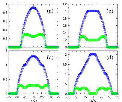
Figure 2: (Color online) Four density profiles ($\triangle$) (cuts across Fig. 1) and their variances ($\bigcirc$). The fillings are $N_{f}=$50 (a), 68 (b), 94 (c), and 150 (d).

Alternatively, Mott-insulating regions can be obtained by increasing the ratio between the on-site repulsive interaction and the hopping parameter as was done in experiments for bosons confined in optical lattices greiner1 . Fig. 3(a) shows the evolution of the density profiles in a trapped system with $N=100$, $N_{f}=70$, and $Va^{2}=0.0025t$ when this ratio is increased from $U/t=2$ to $U/t=8$ [for more details of these density profiles see Fig. 7(e)-7(h)]. It can be seen that for small values of $U/t$ ($U/t=2$) there is only a metallic phase present in the trap. As the value of $U/t$ ($U/t=4$) is increased, a Mott-insulating phase tries to develop at $n=1$ while a metallic phase with $n>1$ is present in the center of the system. As the on-site repulsion is increased even further ($U/t=6,\ 8$), a Mott-insulating domain appears in the middle of the trap suppressing the metallic phase that was present there. In Fig. 3(b) we show the variance of the density for the profiles in Fig. 3(a) (from top to bottom, the values presented are for $U/t=2,\ 4,\ 6,\ 8$). As expected, the variance decreases in both the metallic and Mott-insulating phases when the on-site repulsion is increased. When the Mott-insulating plateau is formed in the density profile, a plateau with constant variance appears in the variance profile with a value that will vanish only in the limit $U/t\rightarrow\infty$. As shown in Fig. 3(b), whenever a Mott-insulating domain is formed in the trap, the value of the variance in it is exactly the same as the one for the Mott-insulating phase in the homogeneous system for the same value of $U/t$ (horizontal dashed lines). This would support the validity of the commonly used local density (Thomas-Fermi) approximation butts97 . However, the insets in Fig. 3(b), show that this is not necessarily the case, since for $U/t=4$, the value of the variance in the Mott-insulating phase of the homogeneous system is still not reached in the trap, although the density reaches the value $n=1$. Therefore, in contrast to the homogeneous case, a Mott-insulating region is not determined by the filling only. In the cases of $U/t=6$ [inset in Fig. 3(b) for a closer look] and $U/t=8$, the value of the variance in the homogeneous system is reached and then we can say that Mott-insulating phases are formed there.

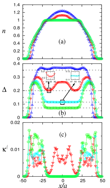
Figure 3: (Color online) Profiles for a trap with $Va^{2}=0.0025t$ and $N_{f}=70$, the on-site repulsions are $U/t=$2 ($\triangle$), 4 ($\bigtriangledown$), 6 ($\Diamond$), and 8 ($\bigcirc$). (a) Local density, (b) variance of the local density, (c) local compressibility $\kappa^{\ell}$ as defined in Eq. (2). The dashed lines in (b) are the values of the variance in the $n=1$ homogeneous system for $U/t=2,\ 4,\ 6,\ 8$ (from top to bottom).

Although the variance gives a first indication for the formation of a local Mott insulator, an ambiguity is still present, since there are metallic regions with densities very close to $n=0$ and $n=2$, where the variance can have even smaller values than in the Mott-insulating phases. Therefore, an unambiguous quantity is still needed to characterize the Mott-insulating regions. We propose a local compressibility as a local-order parameter to characterize the Mott-insulating regions, that is defined as

$$\kappa_{i}^{\ell}=\sum_{\mid j\mid\leq\,\ell(U)}\chi_{i,i+j}\ ,$$ (2)

where

$$\chi_{i,j}=\left\langle n_{i}n_{j}\right\rangle-\left\langle n_{i}\right\rangle\left\langle n_{j}\right\rangle$$ (3)

is the density-density correlation function and $\ell(U)\simeq b\,\xi(U)$, with $\xi(U)$ the correlation length of $\chi_{i,j}$ in the unconfined system at half-filling for the given value of $U$. As a consequence of the charge gap opened in the Mott-insulating phase at half filling in the homogeneous system, the density-density correlations decay exponentially [$\chi_{\left(x\right)}\propto\exp^{-x/\xi\left(U\right)}$] enabling $\xi(U)$ to be determined. The factor $b$ is chosen within a range where $\kappa^{\ell}$ becomes qualitatively insensitive to its precise value. Since there is some degree of arbitrariness in the selection of $b$, we will examine its role in the calculation of $\kappa^{\ell}$ here.

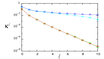
Figure 4: (Color online) Local compressibility as a function of $\ell$ for the homogeneous and trapped ($Va^{2}=0.0025t$, $N_{f}=70$) systems in the Mott-insulating and metallic phases, $U=6t$. ($\bigtriangledown$) $n=1$ homogeneous, ($\bigcirc$) $n_{i=0}=1$ trapped, ($\triangle$) $n=0.66$ homogeneous, and ($\Diamond$) $n_{i=-32}\sim 0.66$ trapped.

We show in Fig. 4 (in a semi-log plot) how the local compressibility behaves as a function of $\ell$ for a homogeneous and a trapped systems in the Mott-insulating ($n=1$) and metallic ($n\sim 0.66$) phases. In the Mott-insulating phase, it is possible to see that in the homogeneous and confined systems the local compressibility decays exponentially to zero in exactly the same way due to the charge gap present there. In the metallic case there is no charge gap so that density-density correlations decay as a power law and the local compressibility, shown in Fig. 4, decays very slowly. In Fig. 4, a departure in the behavior of the local compressibility for the trapped system from the homogeneous case for large values of $\ell$ can be seen. This occurs because correlations with points very close to the band insulating ($n=0$) and the Mott-insulating ($n=1$) regions surrounding the metallic phase [see Fig. 3(a)] are included in $\kappa$. However, this effect does not affect the fact that the value of the local compressibility is clearly different from zero as long as the size of the metallic phase is larger than $2\ell$. We obtain that considering $b\sim 10$ (no matter what the exact value of $b$ is), the local compressibility is zero with exponential accuracy (i.e. $\sim 10^{-6}$ or less) for the Mott-insulating phase and has a finite value in the metallic phase. For the case in Fig. 4 where $U=6t$, the correlation length is $\xi\sim 0.8$ so that $\ell\sim 8$. Physically, the local compressibility defined here gives a measure of the change in the local density due to a constant shift of the potential over a finite range but over distances larger than the correlation length in the unconfined system.

In Fig. 3(c), we show the profiles of the local compressibility for the same parameters as Figs. 3(a) and (b) (we did not include the profile of the local compressibility for $U=2t$ because for that value of $U$ we obtain that $\ell$ is bigger than the system size). In Fig. 3(c), it can be seen that the local compressibility only vanishes in the Mott-insulating domains. For $U=4t$, it can be seen that in the region with $n\sim 1$ the local compressibility, although small, does not vanish. This is compatible with the fact that the variance is not equal to the value in the homogeneous system there, so that although there is a shoulder in the density profile, this region is not a Mott insulator. Therefore, the local compressibility defined here serves as a genuine local order parameter to characterize the insulating regions that always coexist with metallic phases. At this point we would like to remark that, as shown in Ref. rigol1 , the local compressibility shows critical behavior on entering the Mott-insulating region. This is the reason to speak about phases, since on passing from one region to the other, critical behavior sets in.

Finally, we discuss in this section the spin-spin correlation function, since in periodic chains, quasi-long-range antiferromagnetic correlations appear in the Mott-insulating phase. In Fig. 5 we show the local $\langle S^{z}_{i}S^{z}_{j}\rangle$ correlation function for some points of the profiles presented in Fig. 2. We measured the spin-spin correlations in the trap at the points in the figures where it can be clearly seen that $\langle S^{z}_{i}S^{z}_{j}\rangle$ has the maximum value. In Fig. 5(a) it can be seen that in the metallic phase with $n<1$, the spin-spin correlations decay rapidly and do not show any clear modulation, which is due to the fact that the density is changing in this region. In the local Mott-insulating phase [center of the trap in Fig. 5(b)], short-range antiferromagnetic correlations are present, and they disappear completely only on entering in the metallic regions. For the shoulders with $n\sim 1$ [Fig. 5(c)], the antiferromagnetic correlations are still present but due to the small size of these regions they decay very rapidly. Finally for the metallic regions with $n>1$, the spin correlations behave like in the metallic phases with $n<1$ as shown in Fig. 5(d).

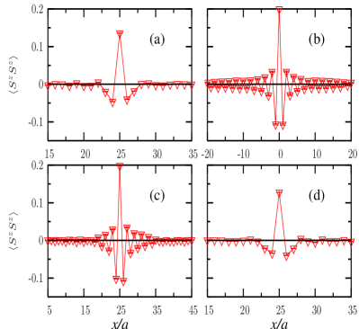
Figure 5: (Color online) Local spin-spin correlations in a trap measured with respect to the points in which in the figure they have their maximum value. The density at each point (total filling in the trap) is $n_{i=25}=0.61$ ($N_{f}=$50) (a), $n_{i=0}=1.00$ ($N_{f}=$68) (b), $n_{i=25}=1.01$ ($N_{f}=$94) (c), and $n_{i=25}=1.44$ ($N_{f}=$150) (d), for a trap with $N=150$, $U=4t$, and $Va^{2}=0.002t$ (the density and variance profiles for these parameters were presented in Fig. 2).

III Momentum distribution function

In most experiments with quantum gases carried out so far, the momentum distribution function, which is determined in time-of-flight measurements, played a central role. A prominent example is given by the study of the superfluid-Mott-insulator transition greiner1 in the bosonic case. Also a QMC study relating this quantity to the density profiles and proposing how to determine the point at which the superfluid-Mott-insulator transition occurs was presented in Ref. kaskurnikov . As shown below, we find that this quantity is not appropriate to characterize the phases of the system in the fermionic case, and does not show any clear signature of the MMIT.

In Fig. 6 we show the normalized momentum distribution function ($n_{k}$) for the same density profiles presented in Fig. 2. For the trapped systems, we always normalize the momentum distribution to be unity at $k=0$. In the case presented in Fig. 6, transitions between phases occur due to changes in the total filling of the trap. We first notice that $n_{k}$ for the pure metallic phase in the harmonic trap [Fig. 6(a)] does not display any sharp feature corresponding to a Fermi surface, in clear contrast to the homogeneous case. The lack of a sharp feature for the Fermi surface is independent of the presence of the interaction and is also independent of the size of the system. In the non-interacting case, this can be easily understood: the spatial density and the momentum distribution will have the same functional form because the Hamiltonian is quadratic in both coordinate and momentum. When the interaction is present, it could be expected that the formation of local Mott-insulating domains generates a qualitatively and quantitatively different behavior of the momentum distribution, like in the homogeneous case where in the Mott-insulating phase the Fermi surface disappears and $n_{k}$ is smoother. In Fig. 6(b), it can be seen that there is no qualitative change of the momentum distribution when the Mott-insulating phase is present in the middle of the trap. Quantitatively $n_{k}$ in this case is very similar to the pure metallic cases Fig. 6(a) (for densities smaller than one) and Fig. 6(c) (where in the middle of the trap the density is higher than one). Only when the insulator with $n=2$ appears in the middle of the system we find a quantitative change of $n_{k}$ for $U=4t$, as shown in Fig. 6(d).

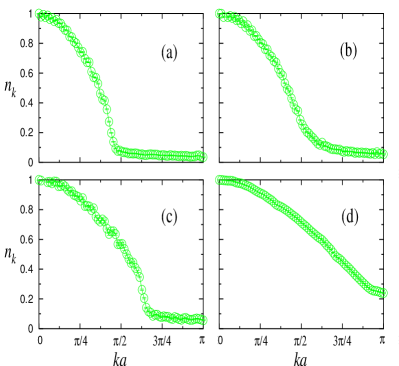
Figure 6: (Color online) Normalized momentum distribution function for the same parameters of Fig. 2. The fillings are $N_{f}=$50 (a), 68 (b), 94 (c), and 150 (d).

We also studied the momentum distribution function when the MMIT is driven by the change of the on-site repulsion. We did not observe any clear signature of the formation of the Mott-insulating phase in $n_{k}$. In Fig. 7 we show the normalized momentum distribution function [Fig. 7(a)-7(d)] for density profiles [Fig. 7(e)-7(h)] in which the on-site repulsion was increased from $U/t=2$ to 8. It can be seen that the same behavior present in Fig. 6 and the quantitative changes in $n_{k}$ appear only when the on-site repulsion goes to the strong-coupling regime, but this is long after the Mott-insulating phase has appeared in the system.

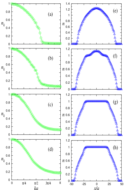
Figure 7: (Color online) Normalized momentum distribution function (a)-(d) and their corresponding density profiles (e)-(h) for $U/t=2$ (a),(e), 4 (b),(f), 6 (c),(g), 8 (d),(h) and $N=100$, $N_{f}=70$, $Va^{2}=0.0025t$.

At this point one might think that in order to study the MMIT using the momentum distribution function, it is necessary to avoid the inhomogeneous trapping potential and use instead a kind of magnetic box with infinitely high potential on the boundaries. However, in that case one of the most important achievements of the inhomogeneous system is lost, i.e., the possibility of creating Mott-insulating phases for a continuous range of fillings. In the perfect magnetic box, the Mott-insulating phase would only be possible at half filling, which would be extremely difficult (if possible at all) to adjust experimentally. The other possibility is to create traps which are almost homogenous in the middle and which have an appreciable trapping potential only close to the boundaries. This can be studied theoretically by considering traps with higher powers of the trapping potentials. As shown below, already non-interacting systems make clear that a sharp Fermi edge is missing in confined systems.

In Fig. 8(a) we show the density profile of a system with 1000 sites, $N_{f}=840$, and a trapping potential of the form $V_{10}x_{i}^{10}$ with $V_{10}a^{10}=7\times 10^{-27}t$. It can be seen that the density is almost flat all over the trap with a density of the order of one particle per site. Only a small part of the system at the borders has the variation of the density required for the particles to be trapped. In Fig. 8(b) (continuous line), we show the corresponding normalized momentum distribution. It can be seen that a kind of Fermi surface develops in the system but for smaller values of $k$, $n_{k}$ is always smooth and its value starts decreasing at $k=0$. In order to see how $n_{k}$ changes when an incompressible region appears in the system, we introduced an additional alternating potential, so that in this case the new Hamiltonian has the form

$$H = -t\sum_{i,\sigma}(c^{\dagger}_{i\sigma}c_{i+1\sigma}+\textrm{H.c.})+V_{10}\sum_{i\sigma}x_{i}^{10}\ n_{i\sigma}$$ (4)

$$+V_{a}\sum_{i\sigma}\left(-1\right)^{i}n_{i\sigma},$$

where $V_{a}$ is the strength of the alternating potential. For the parameters presented in Fig. 8(a), we obtain that a small value of $V_{a}$ ($V_{a}=0.1t$) generates a band insulator in the trap, which extends over the region with $n\sim 1$ (when $V_{a}=0$). However, the formation of this band insulator is barely reflected in $n_{k}$, as can be seen in Fig. 8(b) (dashed line). Only when the value of $V_{a}$ is increased and the system departs from the phase transition [$V_{a}=0.5t$, dotted line in Fig. 8(c)], does a quantitatively appreciable change in $n_{k}$ appear.

Figure 8: Exact results for $N_{f}=840$ noninteracting trapped fermions in a lattice with 1000 sites and a confining potential $V_{10}a^{10}=7\times 10^{-27}t$. Density profile (a) and the normalized momentum distribution function (b): the continuous line corresponds to (a), the dashed line is the result when an alternating potential $V_{a}=0.1t$ is superposed on the system, and the dotted line corresponds to $V_{a}=0.5t$.

In general, it is expected that on increasing the system size, the situation in the homogeneous system is approached. However, in the present case it is not merely a question of boundary conditions, but the whole system is inhomogeneous. Therefore, a proper scaling has to be defined in order to relate systems of different sizes. In the case of particles trapped in optical lattices when there is a confining potential with a power $\alpha$ and strength ($V_{\alpha}$), a characteristic length of the system ($\zeta$) is given by $\zeta=(V_{\alpha}/t)^{-1/\alpha}$, so that a characteristic density ($\tilde{\rho}$) can be defined as $\tilde{\rho}=N_{f}a/\zeta$. We find that this characteristic density is the one meaningful in the thermodynamic limit. In Fig. 9 we show three systems in which the total number of particles and the curvature of the confining potential $V_{10}$ were changed, keeping $\tilde{\rho}$ constant.

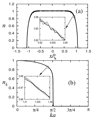
Figure 9: Exact results for noninteracting trapped fermions in a confining potential $V_{10}$. (a) Density profiles, (b) normalized momentum distribution function. Dashed line corresponds to $V_{10}a^{10}=6\times 10^{-24}t$, $N_{f}=428$ ($N\sim 500$), continuous line corresponds to $V_{10}a^{10}=7\times 10^{-27}t$, $N_{f}=840$ ($N\sim 1000$) and dotted line corresponds to $V_{10}a^{10}=1\times 10^{-29}t$, $N_{f}=1620$ ($N\sim 2000$). In the density profiles the positions are given in units of the characteristic length $\zeta$.

We measured the positions in the trap in units of the characteristic length $\zeta$. These systems have occupied regions ($n>0$) with very different sizes, of the order of 500 lattice sites for the dashed line, of the order of 1000 sites for the continuous line, and of the order of 2000 lattice sites for the dotted line. Fig. 9(a) shows that the density profiles scale perfectly when the curvature of the confining potential and the number of fermions are changed in the system, so that in order to show the changes in the density profile, we introduced an inset that expands a region around a density 0.85. In the case of the momentum distribution function [Fig. 9(b)], it is possible to see that this quantity also scales very well so that almost no changes occur in the momentum distribution function when the occupied system size is increased, implying that in the thermodynamic limit the behavior of $n_{k}$ is different from the one in the homogeneous system. An expanded view of the region with $n_{k}$ around 0.87 is introduced to better see the scale of the differences in this region. In Sec. V we show that the characteristic density defined here is also the meaningful quantity to define the phase diagram of the system.

IV Mean-field approximation

The mean-field (MF) approach has been very useful in the study of dilute bosonic gases confined in harmonic potentials dalfovo . This theory for the order parameter associated with the condensate of weakly interacting bosons for inhomogeneous systems takes the form of the Gross-Pitaevskii theory. When the bosonic condensate is loaded in an optical lattice, it is possible to go beyond the weakly interacting regime and reach the strongly correlated limit for which a superfluid-Mott-insulator transition occurs. Also in this limit a MF study was done jaksch , and the results were compared with exact diagonalization results for very small systems, reporting a qualitatively good agreement between both methods jaksch .

In this section, we compare a MF approximation with QMC results for the system under consideration. It will be shown that the MF approach not only violates the Mermin-Wagner theorem, leading to long-range antiferromagnetic order in one dimension, as expected, but also introduces spurious structures in the density profiles. In order to obtain the MF Hamiltonian, we rewrite the Hubbard Hamiltonian in Eq. (1) in the following form (up to a constant shift in the chemical potential):

$$H = -t\sum_{i,\sigma}(c_{i\sigma}^{\dagger}c_{i+1\sigma}+\textrm{H.c.})+V\sum_{i,\sigma}x_{i}^{2}\ \hat{n}_{i\sigma}$$ (5)

$$+\frac{\left(1-\Lambda\right)}{2}[\left\langle\hat{n}_{i}\right\rangle\hat{n}_{i}-\left\langle\hat{n}_{i}\right\rangle^{2}+\widehat{\delta}_{n_{i}}^{2}]$$

$$-\frac{\Lambda}{2}[\left\langle\widehat{\mu}_{i}\right\rangle\widehat{\mu}_{i}-\left\langle\widehat{\mu}_{i}\right\rangle^{2}+\widehat{\delta}_{\mu_{i}}^{2}],$$

where the density and the magnetization in each site are denoted by $\hat{n}_{i}=\hat{n}_{i\uparrow}+\hat{n}_{i\downarrow}$ and $\hat{\mu}_{i}=\hat{n}_{i\uparrow}-\hat{n}_{i\downarrow}$, respectively. The fluctuations of the density and magnetization are given by $\widehat{\delta}_{n_{i}}=\hat{n}_{i}-\left\langle\hat{n}_{i}\right\rangle$ and $\widehat{\delta}_{\mu_{i}}=\hat{\mu}_{i}-\left\langle\hat{\mu}_{i}\right\rangle$, respectively, and $\Lambda$ is an arbitrary parameter that was introduced in order to allow for the most general variation in parameter space. The following relations for fermionic operators were used:

$$\hat{n}_{i\uparrow}\hat{n}_{i\downarrow} = \frac{1}{2}\hat{n}_{i}^{2}-\frac{1}{2}\hat{n}_{i}$$

$$\hat{n}_{i\uparrow}\hat{n}_{i\downarrow} = -\frac{1}{2}\hat{\mu}_{i}^{2}+\frac{1}{2}\hat{n}_{i}.$$ (6)

Neglecting the terms containing the square of the density and magnetization fluctuations in Eq. (5), the following MF Hamiltonian

$$H_{MF} = -t\sum_{i,\sigma}(c_{i\sigma}^{\dagger}c_{i+1\sigma}+\textrm{H.c.})+V\sum_{i,\sigma}x_{i}^{2}\ \hat{n}_{i\sigma}$$ (7)

$$+\frac{1}{2}[\left(1-\Lambda\right)\left\langle\hat{n}_{i}\right\rangle-\Lambda\left\langle\widehat{\mu}_{i}\right\rangle]\hat{n}_{i\uparrow}$$

$$+\frac{1}{2}[\left(1-\Lambda\right)\left\langle\hat{n}_{i}\right\rangle+\Lambda\left\langle\widehat{\mu}_{i}\right\rangle]\hat{n}_{i\downarrow}$$

$$-\frac{\left(1-\Lambda\right)}{2}\left\langle\hat{n}_{i}\right\rangle^{2}+\frac{\Lambda}{2}\left\langle\widehat{\mu}_{i}\right\rangle^{2}$$

is obtained. Due to the inhomogeneity of the trapped system, an unrestricted Hartree-Fock scheme is used to determine the local densities $\left\langle\hat{n}_{i}\right\rangle$ and local magnetic moments $\left\langle\widehat{\mu}_{i}\right\rangle$. Given a MF ground state $|\Psi_{MF}\rangle$, the minimum energy $E=\langle\Psi_{MF}|H|\Psi_{MF}\rangle$ (not the MF one $E_{MF}=\langle\Psi_{MF}|H_{MF}|\Psi_{MF}\rangle$) is reached when $\Lambda=0.5$, so that all the results that follow were obtained for this value of $\Lambda$.

We first recall some of the discrepancies between MF approximations and the known valid facts for the 1D homogenous system ($V=0$) as follows.

(i) At half filling it is known that the Hubbard model exhibits a Mott-insulating phase with a charge gap while the spin sector remains gapless, so that the density-density correlations decay exponentially and the spin-spin correlations decay as a power law. Within the MF approximation, there is a band insulator in the system at half filling so that both the density-density and spin-spin correlations decay exponentially. The MF value of the charge gap is an overestimation of the real one, as can be seen in Fig. 10 where we present the MF results for the density-density correlations as function of the distance, together with the QMC results.

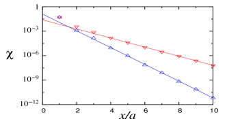
Figure 10: (Color online) Density-density correlations for a homogeneous system with $N=102$ at half filling for $U=6t$. MF ($\triangle$) and QMC ($\bigtriangledown$) solutions.

The slopes of the curves are proportional to the charge gap and the MF slope is approximately twice the QMC one (the results were obtained for a system with 102 sites and $U=6t$). The correlation length of $\chi$ is the inverse of these slopes. Finally, at half filling the MF theory leads to an antiferromagnetic state, while in the Hubbard model the magnetization is always zero although quasi-long-range antiferromagnetic correlations appear in the system.

(ii) At any noncommensurate filling, the Hubbard model in 1D describes a metal (Luttinger liquid), so that no gap appears in the charge and spin excitations, and there is a $2k_{F}$ modulation in the spin-spin correlation function that leads to the well-known $2k_{F}$ singularity. Within the MF approximation, there is always a band insulator at any noncommensurate filling, with a gap that decreases when the system departs from half filling. The appearance of this gap for any density is due to the perfect nesting present in one dimension. The insulating nature of these solutions can be seen in the global compressibility of the system that is always zero, in the behavior of the density-density and the spin-spin correlations which decay exponentially, and in the momentum distribution function where there is no Fermi surface, as shown in Fig. 11 for $N=102$, $N_{f}=66$, and $U=6t$.

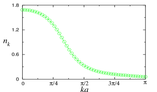
Figure 11: (Color online) MF result for the momentum distribution function of a homogeneous system with $N=102$, $N_{f}=66$, and $U=6t$.

Within this MF approach, there is a $2k_{F}$ modulation of the magnetization only in the $z$ component [the $SU(2)$ symmetry was broken], which leads to a divergence of the Fourier transform of $\langle S^{z}S^{z}\rangle$ at $k=2k_{F}$. In Fig. 12 we compare the MF result (a) for $\langle S^{z}S^{z}\rangle_{k}$ with the QMC one (b), for $N=102$, $N_{f}=66$, and $U=6t$, where it can be seen that the $2k_{F}$ peak is one order of magnitude bigger in the MF case compared to the QMC case. This is due to the existence of the magnetization in the MF solution (the values at the peaks will only diverge in the thermodynamic limit).

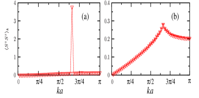
Figure 12: (Color online) MF (a) and QMC (b) results for $\langle S^{z}S^{z}\rangle_{k}$ in a homogeneous system with $N=102$, $N_{f}=66$, and $U=6t$.

We consider next the confined inhomogeneous case. In Fig. 13(a) we show the density profiles obtained for a trap with $N=100$, $N_{f}=70$, and $Va^{2}=0.0025t$ (like the one presented in Fig. 3) for different values of the on-site repulsion $U/t=2,\ 3,\ 4,\ 6$ [for more details see Figs. 15(e)-15(h)]. It can be seen that the MF solutions have also density profiles in which “metallic” ($n\neq 1$) and insulating ($n=1$) phases coexist. However, the MF insulating plateaus with $n=1$ [$U/t=4$ in Fig. 13(a)] appear for smaller values of $U$ than the ones required in the Hubbard model for the formation of the Mott-insulating plateaus [$U/t=6$ in Fig. 3(a)]. In the “metallic” phases it is possible to see that the charge density shows rapid spatial variations that are very large for $n>1,U/t=4$ [see also Fig. 15(f)]. These density variations in the “metallic” phases are reflected in the variance profiles [Fig. 13(b)]. The values of the variance in the plateaus are the same as the ones obtained in the homogeneous MF case for the same value of $U$ when $n=1$ [Fig. 13 (b)]. This feature was discussed in Sec. II for the QMC solutions.

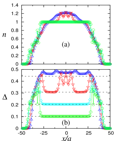
Figure 13: (Color online) MF profiles for a trap with $N=100$, $Va^{2}=0.0025t$, and $N_{f}=70$, the on-site repulsions are $U/t=2$ ($\triangle$), 3 ($\bigtriangledown$), 4 ($\Diamond$), and 6 ($\bigcirc$). (a) Local density, (b) variance of the local density. The dashed lines in (b) are the MF values of the variance in the $n=1$ homogeneous system for $U/t=2,\ 3,\ 4,\ 6$ (from top to bottom).

Since the MF solution leads to an insulating state for incommensurate fillings in the homogeneous case, we analyze in the following more carefully the regions with $n\neq 1$ in the presence of the trap. We find that the local compressibility always decays exponentially as a function of $\ell$ over the entire system, although the exponents are different depending on the density of the point analyzed. Some additional modulation appears in $\kappa^{\ell}$ when $n\neq 1$, as shown in Fig. 14 where the local compressibility is displayed as a function of $\ell$ for $n=1$ and $n\sim 0.66$ in the trapped and homogeneous cases. Therefore, although the MF approximation leads to a density profile similar to the one obtained in QMC as long as $n<1$, it gives a qualitative wrong description of the character of those regions.

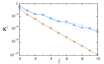
Figure 14: (Color online) MF local compressibility as a function of $\ell$ for the homogeneous and trapped ($Va^{2}=0.0025t$, $N_{f}=70$) systems for $n=1$ and $n\sim 0.66$, $U=6t$. ($\bigtriangledown$) $n=1$ homogeneous, ($\bigcirc$) $n_{i=0}=1$ trapped, ($\triangle$) $n\sim 0.66$ homogeneous, and ($\Diamond$) $n_{i=-30}\sim 0.66$ trapped.

The MF results for the normalized momentum distribution function are presented in Figs. 15(a)-15(d) with their corresponding density profiles [Figs. 15(e)-15(h)], for the same parameter values as in Fig. 13. It can be seen that the normalized momentum profiles are similar to the ones obtained with QMC when the density profiles are similar, so that the MF results are very similar to the QMC ones for this averaged quantity although the physical situation is very different. (Within MF there is always an insulator in the system and within QMC there are metallic and insulating phases coexisting.) In Figs. 15(e)-15(h), we also show the $\langle S^{z}\rangle$ component of the spin on each site of the trap [$S^{z}=\left(\hat{n}_{i\uparrow}-\hat{n}_{i\downarrow}\right)/2$]. When the density is around $n=1$, it can be seen that antiferromagnetic order appears, and that a different modulation exists for $n\neq 1$. We should mention that we have also found some MF solutions for the trapped system where there was formation of spin domain walls in the insulating regions with $n=1$ and there the variance was not constant (a plateau in the density does not correspond to a plateau in the variance), so that care should be taken with the mean field solutions.

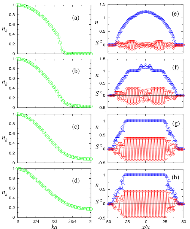
Figure 15: (Color online) MF normalized momentum distribution function ($\bigcirc$) (a)-(d), and their corresponding density ($\triangle$) and $\langle S^{z}\rangle$ ($\bigtriangledown$) profiles (e)-(h) for $U/t=2$ (a),(e), 3 (b),(f), 4 (c),(g), 6 (d),(h) and $N=100$, $N_{f}=70$, $Va^{2}=0.0025t$.

V Phase Diagram

In the present section, we study the phase diagram for fermions confined in harmonic traps with an underlying lattice.

As it can be inferred from Fig. 1, the phases present in the system are very sensitive to the values of the parameters in the model, i.e., to the curvature of the parabolic potential ($V$), to the number of fermions present in the trap ($N_{f}$) and to the strength of the on-site repulsion ($U$). In order to be able to relate systems with different values of these parameters and different sizes, we use the characteristic density ($\tilde{\rho}$) defined in Sec. III for the definition of the phase diagram. This quantity has been shown to be a meaningful quantity in the thermodynamic limit since density profiles (as function of $x/\zeta$) and normalized momentum distributions do not change when $\tilde{\rho}$ is kept constant and the filling in the system (or the occupied system size) is increased. For a harmonic potential, the characteristic length is given by $\zeta=\left(V/t\right)^{-1/2}$ and the characteristic density is then $\tilde{\rho}=N_{f}a\left(V/t\right)^{1/2}$. In Fig. 16 we show the phase diagrams of two systems with different strengths of the confining potential ($Va^{2}=0.006t$ and $Va^{2}=0.002t$) and different sizes ($N=100$ and $N=150$, respectively). This shows that the characteristic density is a meaningful quantity to characterize a generic phase diagram. It allows to compare different systems, and, hence, to relate the results of numerical simulations with larger experimental sizes (although currently the linear dimension of the experiments is $\sim 65\ a$).

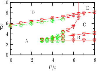
Figure 16: (Color online) Phase diagram for systems with $Va^{2}=0.006t,\ N=100$ ($\bigtriangledown$) and $Va^{2}=0.002t,\ N=150$ ($\bigcirc$). The different phases are explained in the text.

The phases present in the phase diagram in Fig. 16 can be described as follows: (A) a pure metal without insulating regions, (B) a Mott insulator in the middle of the trap always surrounded by a metal, (C) a metallic region with $n>1$ in the center of the Mott-insulating phase, that is surrounded by a metal with $n<1$, (D) an insulator with $n=2$ in the middle of the trap surrounded only by a metallic phase, and finally (E) a “band insulator” in the middle of the trap surrounded by metal with $n>1$, and these two phases inside a Mott insulator that as always is surrounded by a metal with $n<1$. As it can be seen, this phase diagram is more complex than the one for the 1D homogeneous Hubbard model.

There are some features that we find interesting in this phase diagram: (i) For all the values of $U$ that we have simulated, we see that the lower boundary of phase B with the phase A has a constant value of the characteristic density. (ii) We have also seen that the upper boundary of phase B with phases A and C and the boundary of phases D and E with A and C, respectively, are linear within our errors. (iii) Finally, there is another characteristic of phase B, and of the metallic phase A that is below phase B, that we find intriguing and could be related to point (i). As can be seen in Fig. 3(a) for $U/t=6$ and 8, once the Mott-insulating phase is formed in the middle of the trap, a further increase of the on-site repulsion leaves the density profile almost unchanged. (The two mentioned profiles are one on top of the other in that figure.) However, if we look at the variance of these profiles it decreases with increasing $U$, which means that the double occupancy $\left\langle n_{\uparrow}n_{\downarrow}\right\rangle=\left[\Delta-n\left(1-n\right)\right]/2$ is decreasing in the system when $U$ is increased, without a redistribution of the density. Less expected for us is that this also occurs for the metallic phase A that is below phase B. In Fig. 17(a) we show four density profiles and in Fig. 17(b) their variances, for a trap with $Va^{2}=0.006t$ and $N_{f}=30$ when the on-site repulsion has values $U/t=2$, 4, 6, and 8. If we look at the phase diagram, the point with $U/t=2$ is not below phase B whereas the other three values are. In Fig. 17(a) we can see that as the value of $U/t$ is increased from 2 to 4 there is a visible change in the density profile, but after a further increase the profile remains almost the same for the other values of $U$. The inset shows a magnification of the top of the profiles for a more detailed view. Fig. 17(b) shows that although the density stays almost constant for $U/t=4,\ 6$, and 8, the variance decreases. In the other phases (C, D, and E), an increase of the on-site repulsion always changes the local densities pushing particles to the edges of the trap.

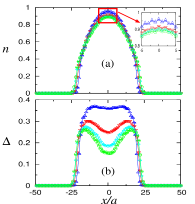
Figure 17: (Color online) Profiles for a trap with $Va^{2}=0.006t$ and $N_{f}=30$, the on-site repulsions are $U/t=2$ ($\triangle$), 4 ($\bigtriangledown$), 6 ($\Diamond$), and 8 ($\bigcirc$). (a) Local density, (b) variance of the local density.

Finally, in order to see, whether the features of the phase diagram discussed previously are particular of a harmonic confining potential, we have also performed an analogous study for a quartic confining potential. In Fig. 18 we show how the density profiles evolve in a trap with a quartic confining potential ($V_{4}a^{4}=3\times 10^{-6}t$) when the total filling is increased from $N_{f}=20$ to 140. It can be seen that the shape of the metallic regions is flatter than in the harmonic case. However, all the features discussed previously for the parabolic confining potential are also present in the quartic case. Local phases appear in the system, the Mott-insulating plateaus with $n=1$ have values of the variance equal to the ones in the homogeneous case for the same value of $U$, the local compressibility vanishes in the Mott-insulating regions and the spin and momentum distribution exhibit a behavior similar to that of the parabolic case.

Figure 18: Evolution of the local density in a quartic confining potential as a function of the position in the trap and increasing total number of fermions. The parameters involved are $N=100$, $U=5t$, and $V_{4}a^{4}=3\times 10^{-6}t$.

In addition, the form of the phase diagram for the quartic confining potential is similar to that of the harmonic trap. In Fig. 19 we show the phase diagram for a system with $N=100$ and $V_{4}a^{4}=3\times 10^{-6}t$, where the characteristic density is given by $\tilde{\rho}=N_{f}a\left(V_{4}/t\right)^{1/4}$. We have also calculated some points of the phase diagram for another system with $V_{4}a^{4}=10^{-6}t$ and $N=100$ in order to check that the scaling relation also works properly in this case. The phases are labeled in the same way as in Fig. 16, up to the largest value of $U$ that we have studied we do not obtain the phase E which for the quartic confining case seems to be moved further towards the strong coupling regime. Figure 19 shows that the phase diagram in this case is very similar to that of the parabolic case, so that all the features discussed previously apply to the quartic confining potential. The form of the phase diagram in Fig. 16 seems to be of general applicability for any confining potential when the proper characteristic density is considered.

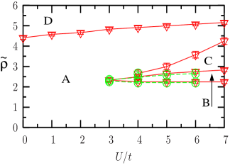
Figure 19: (Color online) Phase diagram for systems with $V_{4}a^{4}=3\times 10^{-6}t,\ N=100$ ($\bigtriangledown$) and $V_{4}a^{4}=10^{-6}t,\ N=100$ ($\bigcirc$). The phases are labeled in the same way as in Fig. 16.

VI Conclusions

We have studied the ground-state properties of the 1D fermionic Hubbard model in harmonic traps with an underlying lattice, using QMC simulations and a MF approach.

Due to the inhomogeneous density distribution, in general metallic and insulating regions coexist in the trap. Therefore, local quantities have to be used to characterize the system. We considered first the variance of the local density, which, when a plateau develops in the density profile with $n=1$, equals the value in the homogeneous system in the Mott-insulating phase. However, it is not an unambiguous quantity, since it can be larger in the Mott-insulating phases than in metallic regions with densities close to $n=0$ or $n=2$. Therefore, we have defined a local-order parameter (local compressibility) that vanishes in the insulating regions and is finite in the metallic ones. The local compressibility gives a measure of the local change in density due to a constant shift of the potential over finite distances larger than the correlation length of the density-density correlation function for the Mott-insulating phase in the unconfined system. As expected, antiferromagnetic correlations are present in the Mott-insulating phases and they remain in the shoulders of the density profile for $n\sim 1$.

As opposed to homogeneous or periodic systems, where the appearance of a gap can in general be seen by the disappearance of the Fermi edge in the momentum distribution function, it is easily seen that due to the presence of a confining potential, such a feature is much less evident. Although increasing the power of the confining potential sharpens the features connected with the Fermi edge, it remains qualitatively different from the homogeneous case. Increasing the system size with a proper definition of the thermodynamic limit, does not change at all the behavior of the density and momentum distribution functions in the trapped case, such that, in fermionic systems it does not seem to be the appropriate quantity to look for evidence of gaps opening in the system.

The MF study has shown that within this approach the trapped system is an insulator for all the densities in the trap, a qualitatively wrong picture in contradiction with the QMC results. In addition, the metallic regions showed large oscillations in the density that are not present in the real solutions. However, it is possible to obtain some qualitative information from MF, such as the coexistence of $n\neq 1$ regions with $n=1$ plateaus, the shape of the momentum distribution function and the existence of antiferromagnetic correlations in the insulating regions with $n=1$.

Finally, we have determined a generic form for the phase diagram that allows to compare systems with different values of all the parameters involved in the model. It can be used to predict the phases that will be present in future experimental results. The phase diagram also reveals interesting features such as reentrant behavior in some phases when some parameters are changed and phase boundaries with linear forms. A similar form of the phase diagram has been also found for a quartic confining potential, such that the results obtained here are generally applicable to cases beyond a perfect harmonic potential.

- (1) M. H. Anderson, J. R. Ensher, M. R. Matthews, C. E. Wieman, and E. A. Cornell, Science 269, 198 (1995).
- (2) C. C. Bradley, C. A. Sackett, J. J. Tollett, and R. G. Hulet, Phys. Rev. Lett. 75, 1687 (1995).
- (3) K. B. Davis, M.-O. Mewes, M. R. Andrews, N. J. van Druten, D. S. Durfee, D. M. Kurn, and W. Ketterle, Phys. Rev. Lett. 75, 3969 (1995).
- (4) Bose-Einstein Condensation in Atomic Gases, Proceedings of the International School of Physics “Enrico Fermi”, edited by M. Inguscio, S. Stringari and C. E. Wieman (IOS Press, Amsterdam, 1999).
- (5) F. Dalfovo, S. Giorgini, L. P. Pitaevskii, and S. Stringari, Rev. Mod. Phys. 71, 463 (1999).
- (6) M. Greiner, O. Mandel, T. Esslinger, T. W. Hänsch, and I. Bloch, Nature (London) 415, 39 (2002).
- (7) M. Greiner, O. Mandel, T. W. Hänsch, and I. Bloch, Nature (London) 419, 51 (2002).
- (8) D. Jaksch, C. Bruder, J. I. Cirac, C. W. Gardiner, and P. Zoller, Phys. Rev. Lett. 81, 3108 (1998).
- (9) G. G. Batrouni, V. Rousseau, R. T. Scalettar, M. Rigol, A. Muramatsu, P. J. H. Denteneer, and M. Troyer, Phys. Rev. Lett. 89, 117203 (2002).
- (10) V. A. Kaskurnikov, N. V. Prokof’ev, and B. V. Svistunov, Phys. Rev. A 66, 031601(R) (2002).
- (11) B. DeMarco and D. S. Jin, Science 285, 1703 (1999).
- (12) A. G. Truscott, K. E. Strecker, W. I. McAlexander, G. B. Partridge, and R. G. Hulet, Science 291, 2570 (2001).
- (13) F. Schreck, L. Khaykovich, K. L. Corwin, G. Ferrari, T. Bourdel, J. Cubizolles, and C. Salomon, Phys. Rev. Lett. 87, 080403 (2001).
- (14) S. R. Granade, M. Gehm, K. M. O’Hora, and J. E. Thomas, Phys. Rev. Lett. 88, 120405 (2002).
- (15) Z. Hadzibabic, C. A. Stan, K. Dieckmann, S. Gupta, M. W. Zwierlein, A. Görlitz, and W. Ketterle, Phys. Rev. Lett. 88, 160401 (2002).
- (16) G. Roati, F. Riboli, G. Modugno, and M. Inguscio, Phy. Rev. Lett. 89, 150403 (2002).
- (17) K. M. O’Hara, S. L. Hemmer, M. E. Gehm, S. R. Granade, and J. E. Thomas, Science 298, 2179 (2002).
- (18) M. Imada, A. Fujimori, and Y. Tokura, Rev. Mod. Phys. 70, 1039 (1998).
- (19) M. Rigol, A. Muramatsu, G. G. Batrouni, and R. T. Scalettar, Phys. Rev. Lett. 91, 130403 (2003).
- (20) G. Sugiyama and S. Koonin, Ann. Phys. (N.Y.) 168, 1 (1986).
- (21) S. Sorella, E. Tosatti, S. Baroni, R. Car, and M. Parrinello, Int. J. Mod. Phys. B 1, 993 (1988).
- (22) D. J. Scalapino and R. L. Sugar, Phys. Rev. Lett. 46, 519 (1981).
- (23) R. Blankenbecler, D. J. Scalapino, and R. L. Sugar, Phys. Rev. D 24, 2278 (1981).
- (24) D. J. Scalapino and R. L. Sugar, Phys. Rev. B 24, 4295 (1981).
- (25) J. E. Hirsch, Phys. Rev. B 28, 4059 (1983).
- (26) A. Muramatsu, in Quantum Monte Carlo Methods in Physics and Chemistry, Vol. 525 of NATO Advanced Studies Institute, Series C: Mathematical and Physical Sciences, edited by M.P. Nightingale and C.J. Umrigar, (NATO Science Series, Kluwer Academic, 1999), pp. 343-373.
- (27) F. F. Assaad, in Quantum Simulations of Complex Many-Body Systems: From Theory to Algorithms, edited by J. Grotendorst, D. Marx, and A. Muramatsu (John von Neumann Institute for Computing (NIC), 2002), Vol. 10, pp. 99-155.
- (28) P. Vignolo, A. Minguzzi, and M. P. Tosi, Phys. Rev. Lett. 85, 2850 (2000).
- (29) D. A. Butts and D. S. Rokhsar, Phys. Rev. A 55, 4346 (1997).