Giant vortices in combined harmonic and quartic traps

Abstract

We consider a rotating Bose-Einstein condensate confined in combined harmonic and quartic traps, following recent experiments [V. Bretin, S. Stock, Y. Seurin and J. Dalibard, cond-mat/0307464]. We investigate numerically the behavior of the wave function which solves the three-dimensional Gross Pitaevskii equation. When the harmonic part of the potential is dominant, as the angular velocities $\Omega$ increases, the vortex lattice evolves into a giant vortex. We also investigate a case not covered by the experiments or the previous numerical works: for strong quartic potentials, the giant vortex is obtained for lower $\Omega$, before the lattice is formed. We analyze in detail the three dimensional structure of vortices.

I Introduction

The existence and formation of quantized vortices have recently been widely studied in Bose Einstein condensates mal ; MCWD2 ; MCWD ; RK ; AK ; RBD . One type of experiments consists in rotating the magnetic trap confining the atoms. For a harmonic trapping potential $(1/2)m\omega_{\perp}^{2}r^{2}$, and a rotating frequency $\Omega$ close to $0.7\omega_{\perp}$, vortices start to appear and arrange themselves into a lattice MCBD . As $\Omega$ is increased, the number of vortices increases as well. In the case of a harmonic trap, the confinement and the centrifugal force prevent the condensate from rotating at a frequency $\Omega$ beyond $\omega_{\perp}$. The regime of fast rotation is especially interesting since it provides a setting for a large number of vortices and eventually giant vortices Fi ; E .

Theoretical and numerical studies have considered stiffer potentials than the harmonic one, behaving like $r^{n}$ or $r^{2}+r^{4}$ F ; L ; K ; Kav . This type of trapping, which eliminates the singular behavior at $\Omega=\omega_{\perp}$, has recently been achieved experimentally by superimposing a blue detuned laser beam to the magnetic trap holding the atoms BD . The resulting potential is

$$V_{trap}(r,z)=V_{h}(r,z)+U(r),$$ (1)

with

$$V_{h}={1\over 2}m\omega^{2}_{\perp}r^{2}+{1\over 2}m\omega^{2}_{z}z^{2},\hbox{ and }U(r)=U_{0}\exp\bigl{(}-{{2r^{2}}\over{w^{2}}}\bigr{)}.$$ (2)

For $r/w$ sufficiently small, the resulting potential can be approximated by :

$$V_{trap}\simeq\left[{1\over 2}m\omega^{2}_{\perp}-{{2U_{0}}\over w^{2}}\right]r^{2}+{{2U_{0}}\over w^{4}}r^{4}+{1\over 2}m\omega^{2}_{z}z^{2}.$$ (3)

The purpose of this paper is to find the stable states (vortex lattice, vortex array with hole and giant vortices) of the condensate with this type of trapping potential and to analyze their three-dimensional structure. We consider a case similar to the experiments and previous theoretical settings, where the amplitude $U_{0}$ of the superimposed laser is small, so that the coefficient of the $r^{2}$ term is positive. But we are especially interested in the case where the laser beam has sufficiently large amplitude so that

$${1\over 2}m\omega^{2}_{\perp}<{{2U_{0}}\over w^{2}}.$$ (4)

This changes the sign of the harmonic part of the potential (3). The point is that, this case of a quartic minus harmonic potential allows to observe giant vortices at lower angular velocities than previously and the structure of vortices is different.

II Numerical approach

We consider a pure BEC of $N$ atoms confined in a trapping potential $V_{trap}$, rotating along the $z$ axis at angular velocity $\Omega$. The equilibrium of the system corresponds to local minima of the Gross-Pitaevskii energy in the rotating frame

$$\displaystyle{\cal E}(\phi) = \displaystyle\int_{\cal D}{\hbar^{2}\over{2m}}|\nabla\phi|^{2}+{{\hbar{\bf\Omega}}}\cdot(i\phi,\nabla\phi\times{\bf x})$$ (5)

$$\displaystyle+V_{trap}\,|\phi|^{2}+{{N\over 2}g_{3D}}|\phi|^{4}$$

where $g_{3D}=4\pi\hbar^{2}a/m$ and the wave function $\phi$ is normalized to unity $\int_{\cal D}|\phi|^{2}=1$.

For numerical purposes, it is convenient to rescale the variables as follows: ${\bf r}={\bf x}/R$, $u({\bf r})=R^{3/2}\phi({\bf x})$, where $R=d/\sqrt{\varepsilon}$ and

$$d=\left(\frac{\hbar}{m\omega_{\perp}}\right)^{1/2},\,\,\varepsilon=\left({{d}\over{8\pi Na}}\right)^{2/5},\,\,{{\tilde{\Omega}}}={\Omega}/{(\varepsilon\omega_{\perp})}.$$ (6)

In this scaling, the trapping potential (3) becomes

$$V=(1-\alpha)r^{2}+{1\over 4}kr^{4}+\beta^{2}z^{2},$$ (7)

where

$$\alpha=\frac{4U_{0}}{m\omega_{\perp}^{2}w^{2}},\quad k=4\alpha\left(\frac{R}{w}\right)^{2},\quad\beta=\frac{\omega_{z}}{\omega_{\perp}}.$$ (8)

Note that we take $\omega_{\perp}$ (which is the frequency of the original harmonic potential $V_{h}$), and not $\omega_{\perp}\sqrt{|1-\alpha|}$, as a scaling frequency for $\Omega$. For numerical applications, we choose $\varepsilon=0.02$, $\beta=\omega_{z}/\omega_{\perp}=1/7$, $k/\alpha=0.25$, which fit the experimental values of Ref. BD . In BD , $\alpha=0.25$, but we will take bigger values since our aim is to understand the influence of $\alpha$ when it gets bigger than 1.

Then, we use the dimensionless energy introduced in AD

$${E}(u)=H(u)-{{\tilde{\Omega}}}L_{z}(u),$$ (9)

where $H$ is the hamiltonian

$$H(u)=\int{1\over 2}|\nabla u|^{2}+{1\over 2\varepsilon^{2}}V|u|^{2}+{1\over 4\varepsilon^{2}}|u|^{4}\;,$$ (10)

and $L_{z}$ the angular momentum axis

$$L_{z}(u)=i\int\bar{u}\left(y\frac{\partial u}{\partial x}-x\frac{\partial u}{\partial y}\right).$$ (11)

Using a hybrid Runge-Kutta-Crank-Nicolson scheme described in Ref. AD , we compute critical points of ${E}(u)$ by solving the norm-preserving imaginary time propagation of the corresponding equation:

$$\frac{\partial u}{\partial t}-{1\over 2}\nabla^{2}u+i({{\tilde{\bf\Omega}}}\times{\bf r}).\nabla u=-{1\over{2\varepsilon^{2}}}u(V+|u|^{2})+\mu_{\varepsilon}u,$$ (12)

where $\mu_{\varepsilon}$ is the Lagrange multiplier for the constraint $\int_{\cal D}|u|^{2}=1$ and with $u=0$ on $\partial{\cal D}$ and. Here, ${\cal D}$ is a rectangular domain containing the condensate. A typical simulation uses a domain $(x,y,z)\in[-2,2]\times[-2,2]\times[-2.8,2.8]$ with a refined grid of $200\times 200\times 140$ nodes, which is sufficient to achieve grid-independence for all considered numerical experiments.

We first compute the steady state corresponding to a nonrotating ($\Omega=0$) condensate, using as initial condition $u=\sqrt{\rho_{\hbox{\tiny TF}}}$, the Thomas-Fermi profile

$$\rho_{\hbox{\tiny TF}}({\bf r})=\rho_{0}+(\alpha-1)r^{2}-{1\over 4}kr^{4}-\beta^{2}z^{2}.$$ (13)

Depending on the choice of $\alpha$, the Thomas-Fermi density profile can display three different shapes, as shown in figure 1.

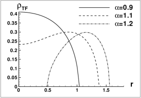
Figure 1: Thomas-Fermi limit $\rho_{\hbox{\tiny TF}}$ for different values of $\alpha$.

The corresponding steady solutions obtained for $\Omega=0$ (which will be used as initial conditions for the subsequent runs with $\Omega>0$) are displayed in figure 2.

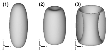
Figure 2: Different shapes of the condensate at $\Omega=0$: isosurfaces of lowest density in the condensate for $\alpha=0.9$ (picture 1), $1.1$ (picture 2), $1.2$ (picture 3).

We can distinguish three cases:

• $\alpha<1$ (weak quartic case) is the case closest to the experiments and is strongly influenced by the harmonic part. For $\Omega=0$, a classical prolate condensate is obtained. As $\Omega$ increases, the effective trapping potential $V^{eff}({\bf r})=V({\bf r})-\varepsilon^{2}\Omega^{2}r^{2}$ starts to have a mexican hat structure. A vortex lattice appears for intermediate values of $\Omega$ and turns into a lattice with a hole for large $\Omega$.

• $\alpha\gtrsim 1$ (intermediate quartic case): the density profile has a depletion close to the center at $\Omega=0$ but no hole. The criterion for this case is

  $$\xi={{\sqrt{\beta}k^{5/4}}\over{\pi(\alpha-1)^{2}}}>1.$$ (14)

  The density profile starts to have a hole for intermediate values of $\Omega$.

• $\alpha>1$ and $\xi<1$ (strong quartic case): the density profile has a hole for all $\Omega$.

III Description of the results

Depending on the values of $\alpha$ and $\Omega$, we observe different types of configurations: vortex free configurations where the amplitude of the wave function takes into account the shape of the effective trapping potential, vortex lattices, vortex arrays with hole and giant vortices.

III.1 Intermediate quartic case ($\alpha=1.1$)

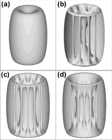
Figure 3: ($\alpha=1.1$) Side view of the condensate for ${\Omega/\omega_{\perp}}=0.12$ (a), $0.2$ (b), $0.28$ (c), $0.32$ (d). Isosurface of lowest density.

The potential $V$ has a Mexican hat structure. The isosurface of lowest density of the solution is plotted in figure 3, the top view in figure 4 and in the middle plane $z=0$ in figure 5. For $\Omega$ small, the density has a depletion close to the center of the condensate but no hole and no vortices. For $\Omega$ larger ($\Omega/\omega_{\perp}\geq 0.16$), vortices are nucleated.

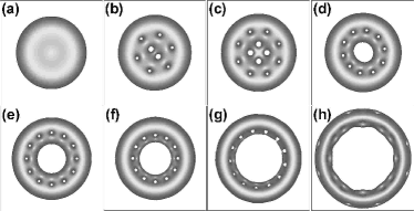
Figure 4: ($\alpha=1.1$) Top view of the condensate for ${\Omega/\omega_{\perp}}=0.12$ (a), $0.16$ (b), $0.2$ (c), $0.24$ (d), $0.28$ (e), $0.32$ (f), $0.4$ (g) and $0.48$ (h). Isosurface of lowest density.

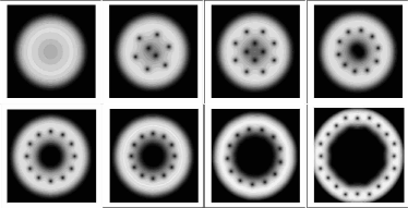
Figure 5: ($\alpha=1.1$) Density contours in the plane $z=0$ for the same states as in figure 4: ${\Omega/\omega_{\perp}}=0.12$, $0.16$, $0.2$, $0.24$, $0.28$, $0.32$, $0.4$ and $0.48$.

For $0.16\leq\Omega/\omega_{\perp}<0.24$, the density of the solution is zero close to the top and bottom of the condensate, but not at the center, which gives rise to a special structure of vortices: the vortices arrange themselves along two concentric circles. The inner circle is made up of vortices which are isolated in the center of the condensate but reconnect towards the top of the condensate (see the details in figure 6). The outer circle is made up of almost straight $U$ vortices that reconnect to the inner circle close to the top and bottom of the condensate. As $\Omega$ increases, the number of vortices on each circle increases. In figure 4(b), the inner vortices seem to be bigger, but this is just an effect due to the projection and the bending: the view at $z=0$ (figure 5) allows to check that all vortices have the same size.

For $\Omega/\omega_{\perp}\geq 0.24$, the density profile of the solution is zero in the center of the condensate, hence this creates a giant vortex: the straight vortices that were close to the center on the inner circle have merged into a giant vortex. There are also isolated vortices regularly scattered on a circle around the giant vortex. As $\Omega$ increases, the number of vortices inside and outside the giant vortex increases and the length of the isolated vortices decreases as can be seen in figure 3.

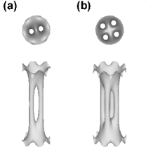
Figure 6: ($\alpha=1.1$) Vortex reconnection details for ${\Omega/\omega_{\perp}}=0.16$ (a), $0.2$ (b).

Note that the isolated vortices are $U$ vortices that reconnect to the giant vortex at the center, not to the boundary of the condensate, as in the case of the harmonic trapping AD , that is their bending is concave not convex.

For $\Omega/\omega_{\perp}=0.48$, (see figure 7) the number of vortices has increased and there are 2 outer circles of vortices around the giant vortex: one circle of $U$ vortices that reconnect to the giant vortex and one circle of vortices that reconnect to the outer boundary of the condensate. Both have different concavity in their bending as illustrated in figure 7.

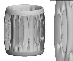
Figure 7: ($\alpha=1.1$) Vortex details for ${\Omega/\omega_{\perp}}=0.48.$

III.2 Strong quartic potential case ($\alpha=1.2$)

The effective potential has a Mexican hat structure for all $\Omega$ and the density profile of the solution always has a hole in the center as illustrated in figure 8.

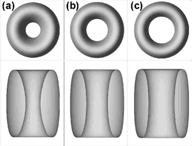
Figure 8: ($\alpha=1.2$) Top and side view of the condensate for ${\Omega/\omega_{\perp}}=0$ (a), $0.12$ (b) and $0.2$ (c).

For small $\Omega$, there are no vortices, that is $L_{z}=0$; it is only the modulus of the solution that goes to zero. For larger $\Omega$ ($\Omega/\omega_{\perp}\geq 0.12$), the hole contains a giant vortex and $L_{z}$ increases with $\Omega$ (see figure 9). We have not found any isolated vortex around the giant vortex: all vortices are included in the central giant vortex because of the strong potential.

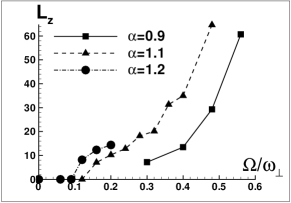
Figure 9: Angular momentum $L_{z}$ (in units of $\hbar$) for all studied configurations.

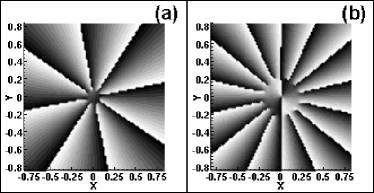
Figure 10: ($\alpha=1.2$) Phase distribution in a central $z=0$ cut plane. ${\Omega/\omega_{\perp}}=0.12$ (a) and $0.2$ (b).

The giant vortex phase profiles (figure 10) show that the phase singularities do not completely overlap in the center of the vortex. This feature has already been observed in two-dimensional numerical simulation of a fast rotating condensate by Kasamatsu et al K . They described the giant vortex as the hole containing single quantized vortices with such low density that they are discernible only by the phase defects.

III.3 Weak quartic case ($\alpha=0.9$)

This is the case closest to the experiments BD . The special feature of this case is that one has to achieve larger values of $\Omega$ in order to obtain giant vortices. The density profile of the solutions are shown in figures 11 and 12.

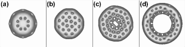
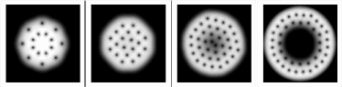
Figure 11: ($\alpha=0.9$) Top view of the condensate (up) and density contours in the plane $z=0$ (down) for $\Omega/\omega_{\perp}=0.32$ (a), $0.4$ (b), $0.48$ (c) and $0.56$ (d).

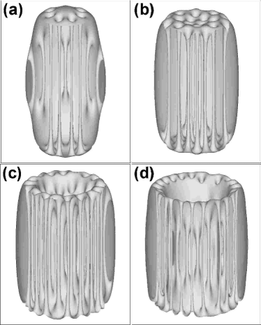
Figure 12: ($\alpha=0.9$) Side view of the condensate for $\Omega/\omega_{\perp}=0.32$ (a), $0.4$ (b), $0.48$ (c) and $0.56$ (d).

Figure 12 show the three dimensional structure of vortices. There are isolated single quantized vortices, forming a lattice. Increasing $\Omega$ leads to a denser lattice (20 vortices for $\Omega/\omega_{\perp}=0.4$ and 38 for $\Omega/\omega_{\perp}=0.48$). As a consequence, the angular momentum (figure 9) grows rapidly to high values.

¿From $\Omega/\omega_{\perp}=0.48$, the vortices near the center of the condensate start to merge, leading to a central structure similar to that displayed in figure 6(a). For $\Omega/\omega_{\perp}\geq 0.56$, the central vortices have merged into a giant vortex. The lattice still exist around. Similarly to the experiments, the hole is obtained for large values of angular velocity ($\Omega/\omega_{\perp}\geq 0.56$).

It is interesting to note from the side view of the condensate (figure 12) that most vortices of the lattice are straight, but some bent vortices (U shape) exist. The U vortices are either connected to the outer boundary (bending outwards) of the condensate (figure 12a,c) or to the giant vortex (bending inwards) (figure 12d).

IV Conclusion

We have studied stable configurations of the Gross Pitaveskii energy when the trapping potential is modified to include a quartic minus a harmonic term.

For weak quartic potentials, the solution evolves from a vortex lattice to a vortex array with hole when the angular velocity $\Omega$ is increased. For stronger quartic potentials, giant vortices are obtained for lower $\Omega$, at a stage where the lattice is not so dense. The typical structure of vortices is to have a central giant vortex with an outer circle of vortices around. We believe that there should be a criterion depending on the radius of the condensate and the radius of the annulus that should characterize the final structure of the giant vortex: whether there is or not a circle of vortices around the giant vortex and its precise location.

The form of the potential considered in our simulations was inspired from recent experiments BD . We have checked that keeping the exponential part of the potential instead of its quartic minus harmonic approximation does not change the qualitative behaviour of the solutions. This suggests that if this situation could be achieved experimentally, it would allow to observe giant vortices for lower velocities than previously, that is before reaching the fast rotation regime.

Acknowledgements: We would like to acknowledge stimulating discussions with V. Bretin.

References

- (1) M. R. Matthews et al., Phys. Rev. Lett., 83, 2498 (1999).
- (2) K. Madison, F. Chevy, V. Bretin and J. Dalibard, Phys. Rev. Lett., 84, 806 (2000).
- (3) K. Madison, F. Chevy, W. Wohlleben and J. Dalibard, J. Mod. Opt., 47, 2715 (2000).
- (4) C. Raman, J. R. Abo-Shaeer, J. M. Vogels, K. Xu, and W. Ketterle, Phys. Rev. Lett. 87, 210402 (2001).
- (5) K. W. Madison, F. Chevy, V. Bretin, and J. Dalibard Phys. Rev. Lett. 86, 4443-4446 (2001).
- (6) J. R. Abo-Shaeer , C. Raman, J. M. Vogels , and W. Ketterle, Science 292, 476 (2001).
- (7) P. Rosenbusch, V. Bretin and J. Dalibard, Phys. Rev. Lett. 89, 200403 (2002)
- (8) U. R. Fischer and G. Baym, Phys. Rev. Lett. 90, 140402 (2003)
- (9) P. Engels, I. Coddington, P. C. Haljan, V. Schweikhard, and E. A. Cornell, Phys. Rev. Lett. 90, 170405 (2003)
- (10) A. L. Fetter, Phys. Rev. A 64, 063608 (2001)
- (11) E. Lundh, Phys. Rev. A 65, 043604 (2002)
- (12) G. M. Kavoulakis and G. Baym, New Jour. Phys. 5, 51.1 (2003)
- (13) K. Kasamatsu, M. Tsubota and M. Ueda, Phys. Rev. A 66, 053606 (2002)
- (14) V. Bretin, S. Stock, Y. Seurin and J. Dalibard, cond-mat/0307464.
- (15) A. Aftalion and I. Danaila, Phys. Rev. A 68, 023603 (2003)