Strong-coupling theory of superconductivity in a degenerate Hubbard model

Abstract

In order to discuss superconductivity in orbital degenerate systems, a microscopic Hamiltonian is introduced. Based on the degenerate model, a strong-coupling theory of superconductivity is developed within the fluctuation exchange (FLEX) approximation where spin and orbital fluctuations, spectra of electron, and superconducting gap function are self-consistently determined. Applying the FLEX approximation to the orbital degenerate model, it is shown that the $d_{x^{2}-y^{2}}$-wave superconducting phase is induced by increasing the orbital splitting energy which leads to the development and suppression of the spin and orbital fluctuations, respectively. It is proposed that the orbital splitting energy is a controlling parameter changing from the paramagnetic to the antiferromagnetic phase with the $d_{x^{2}-y^{2}}$-wave superconducting phase in between.

]

I Introduction

Recently, new heavy fermion superconductors CeTIn₅ (T=Rh, Ir, and Co) have been discovered. These compounds have been atracted much attention, since varieties of ordered states are observed by changing transition metal ions. Among them, CeIrIn₅ and CeCoIn₅ are superconducting at ambient pressure with transition temperatures $T_{\rm c}$=0.4K and 2.3K, respectively.[1, 2] In particular, CeCoIn₅ shows the highest superconducting transition temperature among Ce-based heavy fermion systems. On the other hand, CeRhIn₅ exhibits an antiferromagnetic transition at a Néel temperature $T_{\rm N}$=3.8K and becomes superconducting only under hydrostatic pressure larger than 15 kbar.[3]

The important experimetal results of these materials are summarized as follows. Reflecting the fact that CeTIn₅ has the HoCoGa₅-type tetragonal crystal structure, quasi two-dimensional Fermi surfaces have been observed in de Haas-van Alphen experiments of the compounds, consistent with the band-structure calculations.[4, 5] The specific heat of CeCoIn₅ has shown considerably large discontinity at the superconducting transition temperature by which the superconductivity of this compound is considered to be in the strong-coupling regime.[2] Concerning the superconducting state, nuclear relaxation rate of CeTIn₅ exhibits $T^{3}$ behavior below $T_{\rm c}$[6, 7] and thermal conductivity in CeCoIn₅ is found to show a component with four-fold symmetry,[8] which strongly suggest the $d_{x^{2}-y^{2}}$-wave pairing symmetry of the superconducting phase of CeTIn₅. Furthermore, it has been shown that in the alloy system CeRh_1-xIr_xIn₅, the superconducting phase appears in the neighborhood of the antiferromagnetic phase.[9] These experimental results indicate that the CeTIn₅ compounds have similarity with high-$T_{\rm c}$ cuprates. Thus, it is natural to expect that the mechanism of superconductivity of CeTIn₅ is similar to that of high-$T_{\rm c}$ cuprates.

From the band-structure calculations of CeIrIn₅ and CeCoIn₅, one can see that characteristic features of the Fermi surfaces of these compounds, such as shape, volume, and the $4f$-electron weight, are almost the same with each other.[4, 5, 10] On the other hand, it has been shown in theoretical studies of high-$T_{\rm c}$ cuprates that hole doping leads to the deformation of the Fermi surface and the structure of spin fluctuations around the antiferromagnetic vector is changed. Based on the mechanism of $d_{x^{2}-y^{2}}$-wave superconductivity induced by the antiferromagnetic spin fluctuation, variation of $T_{\rm c}$ in the overdoped region of high-$T_{\rm c}$ cuprates has been explained reasonably by this scenario.[11, 12] It means that hole doping is controlling the superconducting transition temperature through the deformation of the Fermi surface in high-$T_{\rm c}$ cuprates. From the point that the superconducting transition temperatures of CeIrIn₅ and CeCoIn₅ are quite different from each other in spite of the similarities of the Fermi surfaces, it is an improbable scenario that the superconductivity of CeTIn₅ compounds is primarily controlled by the carrier doping as in the high-$T_{\rm c}$ cuprates. Thus, other controlling parameters for the superconductivity should be searched in CeTIn₅ even if the superconducting mechanism of CeTIn₅ is similar to that of high-$T_{\rm c}$ cuprates. In order to find such a controlling parameter of superconductivity in the heavy fermion system CeTIn₅, theoretical study from the microscopic point of view is highly required.

However, theoretical studies for the heavy fermion superconductivity have been almost restricted in the phenomenological level [13] because of the following problems: (1) It is difficult to treat the dual nature of $f$-electrons, coexistence of both localized and itinerant character, in contrast with the $d$-electron systems where the itinerant picture is a good starting point. (2) Complicated $f$-electronic states are formed by the combined effect of crystal structure and orbital degeneracy of $f$-electrons, which leads to multiple Fermi surfaces. For the first difficulty, it may be a reasonable assumption that even strongly correlated states with such a duality of $f$-electrons are still adiabatically continued from the state in weakly correlated systems which is the key assumption of the Fermi-liquid theory. With respect to the second difficulty, it may be appropriate to introduce a microscopic model considering the essential part of the complicated crystal structure. Furthermore, it may be necessary to incorporate the orbital degree of freedom of $f$-electrons into the model, since quasi-particle states are reflected by kinds of orbitals. Thus, in order to understand superconductivity in the heavy fermion system from a microscopic point of view, we should develop a microscopic theory based on the Fermi-liquid type theory using an orbital degenerate model. Especially, in view of the large discontinuity of the specific heat at $T_{\rm c}$ in CeCoIn₅, it is necessary to develop a strong-coupling theory for superconductivity in CeTIn₅ compounds.

In this paper, we focus on the effects of orbital degrees of freedom on superconductivity based on a microscopic theory applied to a microscopic model with the orbital degeneracy. In the next section, we introduce the orbital degenerate model obtained by including important characters of CeTIn₅. Then, in order to study the superconducting transition in the orbital degenerate model, we develop a strong-coupling theory using the fluctuation exchange (FLEX) approximation [14] in which spin and orbital fluctuations, the single-particle spectrum, and superconducting gap function are determined self-consistently. Finally, we discuss experimental results for CeTIn₅ in the light of the present theory.

II Model Hamiltonian

First let us introduce local basis for $f$-electron systems. As is well known, 14-fold degenerate $f$-electronic states split to $j$=5/2 and 7/2 multiplets due to strong spin-orbit coupling where $j$ is total angular momentum. It is quite natural to consider only the lower $j$=5/2 multiplet contributes to low-energy excitations. This multiplet splits into $\Gamma_{7}$ doublet and $\Gamma_{8}$ quartet under cubic crystalline electric field (CEF), and the corresponding eigen-states are given by

$$|\Gamma_{7\pm}\rangle=\sqrt{\frac{1}{6}}|\pm\frac{5}{2}\rangle-\sqrt{\frac{5}{6}}|\mp\frac{3}{2}\rangle,$$ (1)

$$|\Gamma_{8\pm}^{(1)}\rangle=\sqrt{\frac{5}{6}}|\pm\frac{5}{2}\rangle+\sqrt{\frac{1}{6}}|\mp\frac{3}{2}\rangle,$$ (2)

$$|\Gamma_{8\pm}^{(2)}\rangle=|\pm\frac{1}{2}\rangle,$$ (3)

where $|j_{z}\rangle$ are basis of $j$=5/2 multiplet, and $+$($-$) in the subscripts denotes “pseudo-spin” up(down) in each Kramers doublet. Furthermore, under tetragonal CEF, two $\Gamma_{7}$ and one $\Gamma_{6}$ Kramers doublets are formed. Experimental data of magnetic susceptibility of CeTIn₅ analysed by using the CEF theory seem to be consistent with the level scheme where the two $\Gamma_{7}$ are lower than the $\Gamma_{6}$. [15, 16]

Here we consider that superconductivity in systems with the orbital degrees of freedom is affected primarily by splitting enegry between lowest and excited states, while kind of excited Kramers doublet may play secondary role to determine details of electronic properties. Based on this belief, in the following, we consider only $|\Gamma_{8}\rangle$ states. In other words, one $\Gamma_{7}$ state is assumed to be the highest energy state. Note that $|\Gamma_{8\pm}^{(1)}\rangle$ and $|\Gamma_{8\pm}^{(2)}\rangle$ belong to $\Gamma_{7}$ and $\Gamma_{6}$ irreducible representations, respectively, in the tetragonal system. Although this assumption is not exactly the same as the level scheme obtained from experimental results mentioned above, using $\Gamma_{6}$ and $\Gamma_{7}$ states instead of two $\Gamma_{7}$ states will provide even reasonable result to discuss superconductivity of CeTIn₅. [17] We stress that the Hamiltonian constructed from $\Gamma_{8}$ quartet is the simplest possible model including essential physics of interplay between pseudo-spin and orbital degrees of freedom.

We include itinerant features of $f$-electrons by considering nearest-neighbor hopping of $f$-electrons. Since realistic effective hopping of $f$-electrons includes that through hybridization with conduction electrons, such effects may be renormalized to the nearest-neighbor hopping of $f$-electrons after the conduction electron degrees of freedom are integrated out. In the present case, the matrix elements of the hoppings depend on not only the hopping directions but also kinds of orbitals, since the forms of the wave functions of $|\Gamma_{8\pm}^{(1)}\rangle$ and $|\Gamma_{8\pm}^{(2)}\rangle$ states are different from each other. Noting that CeTIn₅ has a tetragonal crystal structure and quasi two-dimensional Fermi surfaces have been experimentally observed, [4, 5] it is natural to consider the two-dimensional square lattice composed of Ce³⁺ ions. Considering these points, we have estimated the hopping matrix elements through the $\sigma$-bond ($ff\sigma$) using the tight-binding method. [10, 18] The matrix elements of nearest-neighbor hopping of $f$-electrons $t^{\bf a}_{\tau\tau^{\prime}}$ between $\tau$ and $\tau^{\prime}$ orbitals along the ${\bf a}$-direction are given by

$$t^{\bf x}_{11}=-\sqrt{3}t^{\bf x}_{12}=-\sqrt{3}t^{\bf x}_{21}=3t^{\bf x}_{22}=t,$$ (4)

for ${\bf a}$=${\bf x}$, and

$$t^{\bf y}_{11}=\sqrt{3}t^{\bf y}_{12}=\sqrt{3}t^{\bf y}_{21}=3t^{\bf y}_{22}=t,$$ (5)

for ${\bf a}$=${\bf y}$. [19] We use $t$=1 as energy unit in the following.

By further adding the on-site Coulomb interaction terms among $f$-electrons, an effective Hamiltonian of CeTIn₅ compounds with orbital degrees of freedom is obtained as

$$H = \sum_{{\bf ia}\tau\tau^{\prime}\sigma}t^{\bf a}_{\tau\tau^{\prime}}f_{{\bf i}\tau\sigma}^{{\dagger}}f_{{\bf i+a}\tau^{\prime}\sigma}-\Delta\sum_{\bf i}(n_{{\bf i}1\sigma}-n_{{\bf i}2\sigma})/2$$ (6)

$$+ U\sum_{{\bf i}\tau}n_{{\bf i}\tau\uparrow}n_{{\bf i}\tau\downarrow}+U^{\prime}\sum_{{\bf i}\sigma\sigma^{\prime}}n_{{\bf i}1\sigma}n_{{\bf i}2\sigma^{\prime}},$$ (7)

where $f_{{\bf i}\tau\sigma}$ is the annihilation operator for an $f$-electron with pseudo-spin $\sigma$ in the $\tau$-orbital state $\Gamma_{8}^{(\tau)}$ at site ${\bf i}$, ${\bf a}$ is the vector connecting nearest-neighbor sites, and $n_{{\bf i}\tau\sigma}$=$f_{{\bf i}\tau\sigma}^{{\dagger}}f_{{\bf i}\tau\sigma}$. The first term represents the nearest-neighbor hopping of $f$-electrons. The second term expresses the tetragonal CEF, represented by an energy splitting $\Delta$ between the two orbitals. In the third and fourth terms, $U$ and $U^{\prime}$ are the intra- and inter-orbital Coulomb interactions, respectively. We ignore the Hund’s rule coupling, since it may be irrelevant for the quarter-filling case with one $f$-electron per site. To keep the rotational invariance in the orbital space for the interaction part of the Hamiltonian, $U^{\prime}$ should be equal to $U$ when we ignore the Hund’s rule coupling. Thus, in this paper, we restrict ourselves to the case of $U$=$U^{\prime}$.

Considering property of the hopping matrix element, [19] the present Hamiltonian in the quarter-filling may be regarded as an effective model in the hole-picture for the CuO₂ plane of a parent compound of high-$T_{\rm c}$ cuprate La₂CuO₄, although the practical value of $\Delta$ may be considerably large for the $d$-electron system. This fact means that some of the results obtained by using the present Hamiltonian can be used for the cuprate with a suitable choice of the parameter set. We also note that in the quarter-filling case, the present model is reduced to a half-filled single-orbital Hubbard model in the limit of $\Delta$=$\infty$.

Here we briefly discuss symmetry properties of the present Hamiltonian. Since all pseudo-spin operators $S^{\alpha}=(1/2)\sum_{{\bf i},\tau}\sum_{\sigma,\sigma^{\prime}}f_{{\bf i}\tau\sigma}^{{\dagger}}\tau^{\alpha}_{\sigma\sigma^{\prime}}f_{{\bf i}\tau\sigma^{\prime}}$ ($\alpha$=$x$, $y$, $z$) with $\hat{\tau}^{\alpha}$ being the Pauli matrices commute with this Hamiltonian, the system is invariant with respect to the rotation in the pseudo-spin space. Since the Hamiltonian is consisted of the pairs of creation and annihilation operators corresponding to each Kramers doublet, it is easily confirmed that the Hamiltonian is invariant under the time reversal. Since we consider the system of two-dimensional square lattice composed of Ce³⁺-ion, the Hamiltonian commutes with all elements of the $D_{4h}$ point group. Obviously, the Hamiltonian is $U(1)$-gauge invariant. Thus, the Hamiltonian has the symmetry of $D_{4h}\times SU(2)\times\Theta\times U(1)$ after all where $SU(2)$ describes the rotation group in the pseudo-spin space and $\Theta$ the time reversal symmetry. In the following, we call pseudo-spin as “spin” for simplicity.

III Formulation

In our previous work, we have developed a weak-coupling theory for superconductivity based on the same orbital degenerate model described above, using the static spin and orbital fluctuations obtained within the random phase approximation (RPA). [20] On the other hand, considerably large discontinuity of the specific heat at the superconducting transition temperature has been observed in CeCoIn₅. [2] Since the discontinuity is much larger than the specific heat just above the superconducting transition temperature, the mass enhancement due to the strong interaction between $f$-electrons may not be responsible for the large discontinuity. Rather, this experimental fact seems to require the strong-coupling theory in order to understand the superconductivity in CeTIn₅ compounds. Thus, we should develop a strong-coupling theory for superconductivity based on the orbital degenerate model.

In the present paper, we apply the fluctuation exchange (FLEX) approximation [14] to the orbital degenerate model discussed in the preceding section. The FLEX approximation provides the Dyson-Gorkov equation where the normal and anomalous self-energies are obtained on an equal footing, namely a kind of the strong-coupling theory. Here, it should be noted that the strong-coupling theory includes two major changes for the orbital degenerate system compared with the single orbital case. One is multi-component nature of the superconducting order parameters in the orbital space, namely orbital symmetric and orbital antisymmetric gap functions. The other is the effect of mode-mode coupling among spin and orbital fluctuations. We expect that the mode-mode coupling significantly affects the temperature and frequency dependences of spin and orbital fluctuations. Therefore, in order to discuss superconductivity induced by these fluctuations the mode-mode coupling effect is very important. In the following, first we discuss general relations satisfied by the Green’s functions required from the symmetry of the system, then develop the scheme of the FLEX approximation for the degenerate model.

A Definition and Properties of Green’s Function

The normal Green’s functions $G^{\sigma}_{mn}({\bf k},\tau)$ describing the propagating process of electrons from $n$-orbital to $m$-orbital with moment ${\bf k}$ and spin $\sigma$ and the anomalous ones $F^{\sigma\sigma^{\prime}}_{mn}({\bf k},\tau)$ and $\overline{F}^{\sigma\sigma^{\prime}}_{mn}({\bf k},\tau)$ describing the superconducting condensation are defined as

$$G^{\sigma}_{mn}({\bf k},\tau)=-\langle T_{\tau}[f_{{\bf k}m\sigma}(\tau)f_{{\bf k}n\sigma}^{{\dagger}}(0)]\rangle,$$ (8)

$$F^{\sigma\sigma^{\prime}}_{mn}({\bf k},\tau)=-\langle T_{\tau}[f_{{\bf k}m\sigma}(\tau)f_{-{\bf k}n\sigma^{\prime}}(0)]\rangle,$$ (9)

$$\overline{F}^{\sigma\sigma^{\prime}}_{mn}({\bf k},\tau)=-\langle T_{\tau}[f_{-{\bf k}m\sigma}^{{\dagger}}(\tau)f_{{\bf k}n\sigma^{\prime}}^{{\dagger}}(0)]\rangle,$$ (10)

where $f_{{\bf k}m\sigma}(\tau)=e^{(H-\mu N)\tau}f_{{\bf k}m\sigma}e^{-(H-\mu N)\tau}$ with $\tau$ being the imaginary time, $N=\sum_{{\bf i},m,\sigma}f_{{\bf i}m\sigma}^{{\dagger}}f_{{\bf i}m\sigma}$ is an operator of the $f$-electron number, $\mu$ the chemical potential, and $T_{\tau}$ describes the time ordered product. In these equations, $\langle\cdots\rangle$ means the thermodynamical average. It is convenient to transform the imaginary time Green’s functions to the frequency representation given by

$${\cal G}({\bf k},{\rm i}\omega_{l})=\int^{1/T}_{0}d\tau\hskip 2.84526pte^{{\rm i}\omega_{l}\tau}{\cal G}({\bf k},\tau),$$ (11)

where ${\cal G}({\bf k},\tau)$ represents a component of the normal or anomalous Green’s functions defined above, and $\omega_{l}$=$(2l+1)\pi T$ is the Matsubara frequency for fermions.

Then, under the assumption that the superconducting transition does not break the time reversal symmetry for the orbital degenerate system, Green’s functions satisfy the relations as

$$G^{\sigma}_{mn}({\bf k},{\rm i}\omega_{l})=G^{\sigma}_{nm}({\bf k},-{\rm i}\omega_{l})^{\ast}=G^{\overline{\sigma}}_{nm}(-{\bf k},{\rm i}\omega_{l}),$$ (13)

$$F^{\sigma\sigma^{\prime}}_{mn}({\bf k},{\rm i}\omega_{l})=-F^{\sigma^{\prime}\sigma}_{nm}(-{\bf k},-{\rm i}\omega_{l})$$

$$= \sigma\sigma^{\prime}F^{\overline{\sigma}\overline{\sigma^{\prime}}}_{mn}(-{\bf k},-{\rm i}\omega_{l})^{\ast}=\sigma\sigma^{\prime}\overline{F}^{\overline{\sigma^{\prime}}\overline{\sigma}}_{nm}(-{\bf k},{\rm i}\omega_{l}),$$ (14)

where the last equalities in these relations are obtained by the time reversal invariance. Due to the $SU(2)$-symmetry in the spin space, $F^{\sigma\sigma^{\prime}}_{mn}({\bf k},{\rm i}\omega_{l})$ are decomposed into the spin-singlet and spin-triplet irreducible representations, defined as

$$F^{\rm s}_{mn}({\bf k},{\rm i}\omega_{l})=\frac{1}{2}(F^{\uparrow\downarrow}_{mn}({\bf k},{\rm i}\omega_{l})-F^{\downarrow\uparrow}_{mn}({\bf k},{\rm i}\omega_{l})),$$ (15)

and

$$F^{\rm t}_{mn}({\bf k},{\rm i}\omega_{l})=\frac{1}{2}(F^{\uparrow\downarrow}_{mn}({\bf k},{\rm i}\omega_{l})+F^{\downarrow\uparrow}_{mn}({\bf k},{\rm i}\omega_{l})),$$ (16)

where $F^{\rm t}_{mn}({\bf k},{\rm i}\omega_{l})$ defined above is a representative of the three components of the spin-triplet pairs. In the paramagnetic system, since we can suppress a superscript describing spin state of $G^{\sigma}_{mn}({\bf k},{\rm i}\omega_{l})$, we obtain the relations for the normal Green’s functions as

$$G_{mn}({\bf k},{\rm i}\omega_{l})=G_{nm}({\bf k},-{\rm i}\omega_{l})^{\ast}=G_{nm}({\bf k},{\rm i}\omega_{l}).$$ (17)

Furthermore, when the orbitals are defined at the Bravais lattice, the inversion operation changes only the wave vector $\bf k$ to -$\bf k$ independent on the orbital state as well as spin of the quasi-particles forming the Cooper pair. Thus, we obtain the relations for $F^{\xi}_{mn}({\bf k},{\rm i}\omega_{l})$ ($\xi$=s or t) as

$$F^{\xi}_{mn}({\bf k},{\rm i}\omega_{l})=F^{\xi}_{mn}({\bf k},-{\rm i}\omega_{l})^{\ast}=F^{\xi}_{nm}({\bf k},{\rm i}\omega_{l})^{\ast}.$$ (18)

Among $F^{\uparrow\downarrow}_{mn}({\bf k},{\rm i}\omega_{l})$, $\overline{F}^{\downarrow\uparrow}_{mn}({\bf k},{\rm i}\omega_{l})$, and $F^{\xi}_{mn}({\bf k},{\rm i}\omega_{l})$, we also obtain

$$F^{\xi}_{mn}({\bf k},{\rm i}\omega_{l})=F^{\uparrow\downarrow}_{mn}({\bf k},{\rm i}\omega_{l})=\overline{F}^{\downarrow\uparrow}_{nm}({\bf k},{\rm i}\omega_{l}).$$ (19)

Note that these relations are obtained in the time reversal invariant system regardless of the spin-singlet and even-parity pair or the spin-triplet and odd-parity pair. We emphasize that these relations are quite useful to make the formulation simple.

By transforming $F^{\xi}_{mn}({\bf k},{\rm i}\omega_{l})$ ($\xi$=s or t) to the “orbital-symmetric” and “orbital-antisymmetric” representations, four real anomalous Green’s functions are defined as

$$F^{\xi}_{1}({\bf k},{\rm i}\omega_{l})\equiv F^{\xi}_{11}({\bf k},{\rm i}\omega_{l}),$$ (20)

$$F^{\xi}_{2}({\bf k},{\rm i}\omega_{l})\equiv F^{\xi}_{22}({\bf k},{\rm i}\omega_{l}),$$ (21)

$$F^{\xi}_{3}({\bf k},{\rm i}\omega_{l})\equiv\frac{1}{\sqrt{2}}(F^{\xi}_{12}({\bf k},{\rm i}\omega_{l})+F^{\xi}_{21}({\bf k},{\rm i}\omega_{l})),$$ (22)

$$F^{\xi}_{4}({\bf k},{\rm i}\omega_{l})\equiv\frac{\rm i}{\sqrt{2}}(F^{\xi}_{12}({\bf k},{\rm i}\omega_{l})-F^{\xi}_{21}({\bf k},{\rm i}\omega_{l})),$$ (23)

where $F^{\xi}_{4}({\bf k},{\rm i}\omega_{l})$ just describes the orbital-antisymmetric pairing. For the spin-singlet state, they satisfy the relations as

$$F^{\rm s}_{m}({\bf k},{\rm i}\omega_{l})=F^{\rm s}_{m}(-{\bf k},{\rm i}\omega_{l})=F^{\rm s}_{m}({\bf k},-{\rm i}\omega_{l}),$$ (24)

$$F^{\rm s}_{4}({\bf k},{\rm i}\omega_{l})=F^{\rm s}_{4}(-{\bf k},{\rm i}\omega_{l})=-F^{\rm s}_{4}({\bf k},-{\rm i}\omega_{l}),$$ (25)

and for the spin-triplet state, we obtain

$$F^{\rm t}_{m}({\bf k},{\rm i}\omega_{l})=-F^{\rm t}_{m}(-{\bf k},{\rm i}\omega_{l})=F^{\rm t}_{m}({\bf k},-{\rm i}\omega_{l}),$$ (26)

$$F^{\rm t}_{4}({\bf k},{\rm i}\omega_{l})=-F^{\rm t}_{4}(-{\bf k},{\rm i}\omega_{l})=-F^{\rm t}_{4}({\bf k},-{\rm i}\omega_{l}),$$ (27)

where $m$ represents the number of the orbital-symmetric component, namely $m$=1, 2, or 3. One can see that the orbital-antisymmetric anomalous Green’s function has odd-frequency dependence, irrespective of the spin state of the Cooper-pair. Thus, due to the odd-frequency property, the orbital-antisymmetric component of the Cooper pair may not provide essential contribution to superconductivity. In addition to this feature in the frequency space, we should also pay attention to the $\bf k$-dependences of $F^{\xi}_{mn}({\bf k},{\rm i}\omega_{l})$ because the lattice system and the local wave functions should be rotated simultaneously. For example, a symmetry operation $C_{4}$ of the tetragonal point group rotates the wave vector ${\bf k}$, and also changes the sign of only the $\Gamma_{7}$ wave function of $f$-electron. The latter effect of the symmetry operation leads to the difference between $\bf k$-dependences of the orbital-diagonal and the orbital-offdiagonal anomalous Green’s functions, in order to preserve the symmetry of superconductivity. After all, when the superconducting state belongs to $\Gamma$ irreducible representation, the $\bf k$-dependences of $F^{\xi}_{12}({\bf k},{\rm i}\omega_{l})$ and $F^{\xi}_{21}({\bf k},{\rm i}\omega_{l})$ have the $\Gamma\times B_{\rm 1g}$-symmetry while the symmetry properties of $F^{\xi}_{11}({\bf k},{\rm i}\omega_{l})$ and $F^{\xi}_{22}({\bf k},{\rm i}\omega_{l})$ in the $\bf k$-space behave as the $\Gamma$ irreducible represenation, the same as the symmetry of the order parameter. These relations obtained in this subsection are useful for practical calculations.

Here we comment on difference between the strong- and weak-coupling theories for the degenerate model. As will be obtained below, the superconducting gap functions are not independent for the orbital-symmetric and orbital-antisymmetric parts generally. On the other hand, in the weak-coupling theory of the same degenerate model, the orbital-symmetric components and the orbital-antisymmetric one of $\Sigma^{\xi(2)}_{mn}(k)$ define separate superconducting states from each other. [20] Considering the result in the present subsection, the complete separation within the weak-coupling theory is due to ignoring the odd-frequency dependence of the orbital-antisymmetric component of the anomalous Green’s functions $F^{\xi}_{4}({\bf k},{\rm i}\omega_{l})$.

B FLEX Approximation for the Degenerate Model

In order to develop a strong-coupling theory of superconductivity in the degenerate system, it is convenient to introduce the Dyson-Gorkov equations, which is in the matrix form because of the orbital degree of freedom, given by

$$\hat{G}(k)=\hat{G}^{(0)}(k)+\hat{G}^{(0)}(k)\hskip 2.84526pt\hat{\Sigma}^{(1)}(k)\hskip 2.84526pt\hat{G}(k)$$ (28)

$$\hskip 69.70924pt+\hat{G}^{(0)}(k)\hskip 2.84526pt\hat{\Sigma}^{\xi(2)}(k)\hskip 2.84526pt\hat{F}^{\xi}(k)^{\rm t},$$ (29)

$$\hat{F}^{\xi}(k)=\hat{G}^{(0)}(k)\hskip 2.84526pt\hat{\Sigma}^{(1)}(k)\hskip 2.84526pt\hat{F}^{\xi}(k)$$ (30)

$$\hskip 32.72066pt-\hat{G}^{(0)}(k)\hskip 2.84526pt\hat{\Sigma}^{\xi(2)}(k)\hskip 2.84526pt\hat{G}(-k)^{\rm t},$$ (31)

where $\hat{\Sigma}^{(1)}(k)$ is a matrix of the normal self-energies, $\hat{\Sigma}^{\xi(2)}(k)$ describes a matrix of the anomalous self-energies for the spin-$\xi$ state pairing and the abbreviation $k\equiv({\bf k},{\rm i}\omega_{l})$ is used. $\hat{G}^{(0)}(k)$ is the matrix of the noninteracting Green’s function whose matrix elements are given by

$$G^{(0)}_{mn}({\bf k},{\rm i}\omega_{l})=\sum_{p}\alpha_{{\bf k}pm}\alpha_{{\bf k}pn}\frac{1}{{\rm i}\omega_{l}-E_{{\bf k}p}}$$ (32)

with

$$E_{{\bf k}p}=\frac{\epsilon_{{\bf k}11}+\epsilon_{{\bf k}22}}{2}+(-1)^{p}\sqrt{\frac{(\epsilon_{{\bf k}11}-\epsilon_{{\bf k}22})^{2}}{4}+\epsilon_{{\bf k}12}^{2}},$$ (33)

$$\alpha_{{\bf k}11}=\alpha_{{\bf k}22}=\left[1+\frac{E_{{\bf k}2}-\epsilon_{{\bf k}11}}{E_{{\bf k}2}-\epsilon_{{\bf k}22}}\right]^{-1/2},$$ (34)

$$\alpha_{{\bf k}12}=-\alpha_{{\bf k}21}=\frac{\epsilon_{{\bf k}12}}{E_{{\bf k}2}-\epsilon_{{\bf k}22}}\alpha_{{\bf k}11},$$ (35)

and

$$\epsilon_{{\bf k}11}=2\hskip 2.84526ptt\hskip 2.84526pt(\cos{k_{x}}+\cos{k_{y}})-\frac{\Delta}{2}-\mu,$$ (36)

$$\epsilon_{{\bf k}22}=\frac{2}{3}\hskip 2.84526ptt\hskip 2.84526pt(\cos{k_{x}}+\cos{k_{y}})+\frac{\Delta}{2}-\mu,$$ (37)

$$\epsilon_{{\bf k}12}=\epsilon_{{\bf k}21}=-\frac{2}{\sqrt{3}}\hskip 2.84526ptt\hskip 2.84526pt(\cos{k_{x}}-\cos{k_{y}}),$$ (38)

where $E_{{\bf k}p}$ is the energy dispersion of $p$-th band and $\alpha_{{\bf k}pm}$ is the weight of $m$-th orbital for the $p$-th band at wave vector ${\bf k}$.

In order to obtain a concrete form of the matrix elements of the self-energy for the degenerate model, we adopt the FLEX approximation. First, we define a “Luttinger-Ward” functional $\Phi[{\cal G}(k)]$ consisting of ladder and bubble diagrams for particle-hole processes but ignoring particle-particle processes, and then generate matrix elements of the self-energy by functional differentiation of $\Phi[{\cal G}(k)]$ with respect to ${\cal G}(k)$ where ${\cal G}(k)$ represents a component of the normal and/or anomalous Green’s functions. By this procedure, the self-energies are obtained within the FLEX approximation by

$$\Sigma^{(1)}_{mn}(k)=\frac{T}{N_{0}}\sum_{q}\sum_{\mu\nu}T^{\rm eff}_{\mu m,\nu n}(q)G_{\mu\nu}(k-q),$$ (39)

and

$$\Sigma^{\xi(2)}_{mn}(k)=\frac{T}{N_{0}}\sum_{q}\sum_{\mu\nu}T^{\xi}_{\mu m,n\nu}(q)F^{\xi}_{\mu\nu}(k-q),$$ (40)

where an abbreviation $q\equiv({\bf q},{\rm i}\Omega_{l})$ is used with the boson Matsubara frequency $\Omega_{l}$=$2l\pi T$. The fluctuation exchange interactions used in $\Sigma^{(1)}_{mn}(k)$ are given by

$$T^{\rm eff}_{\mu m,\nu n}(q)=\frac{1}{2}[3\hat{U}^{\rm s}\hat{\chi}^{\rm s}(q)\hat{U}^{\rm s}+\hat{U}^{\rm o}\hat{\chi}^{\rm o}(q)\hat{U}^{\rm o}$$ (41)

$$\hskip 5.69054pt-\frac{1}{2}(\hat{U}^{\rm s}+\hat{U}^{\rm o})\hat{\overline{\chi}}^{\sigma\sigma}(q)(\hat{U}^{\rm s}+\hat{U}^{\rm o})+3\hat{U}^{\rm s}-\hat{U}^{\rm o}]_{\mu m,\nu n}.$$ (42)

For the spin-singlet channel, matrix elements of the effective pairing interaction are given by

$$T^{\rm s}_{\mu m,n\nu}(q)=\frac{1}{2}[3\hat{U}^{\rm s}\hat{\chi}^{\rm s}(q)\hat{U}^{\rm s}-\hat{U}^{\rm o}\hat{\chi}^{\rm o}(q)\hat{U}^{\rm o}$$ (43)

$$\hskip 5.69054pt+\frac{1}{2}(\hat{U}^{\rm s}+\hat{U}^{\rm o})\hat{\overline{\chi}}^{\sigma\overline{\sigma}}(q)(\hat{U}^{\rm s}+\hat{U}^{\rm o})+\hat{U}^{\rm s}+\hat{U}^{\rm o}]_{\mu m,n\nu},$$ (44)

and for the spin-triplet channel, we obtain

$$T^{\rm t}_{\mu m,n\nu}(q)=\frac{1}{2}[-\hat{U}^{\rm s}\hat{\chi}^{\rm s}(q)\hat{U}^{\rm s}-\hat{U}^{\rm o}\hat{\chi}^{\rm o}(q)\hat{U}^{\rm o}$$ (45)

$$\hskip 5.69054pt+\frac{1}{2}(\hat{U}^{\rm s}+\hat{U}^{\rm o})\hat{\overline{\chi}}^{\sigma\overline{\sigma}}(q)(\hat{U}^{\rm s}+\hat{U}^{\rm o})+\hat{U}^{\rm s}+\hat{U}^{\rm o}]_{\mu m,n\nu},$$ (46)

with

$$\hat{U}^{\rm s}=\left[\begin{array}[]{cccc}U&0&0&0\\ 0&U&0&0\\ 0&0&U^{\prime}&0\\ 0&0&0&U^{\prime}\end{array}\right],\hskip 2.84526pt\hat{U}^{\rm o}=\left[\begin{array}[]{cccc}U&2U^{\prime}&0&0\\ 2U^{\prime}&U&0&0\\ 0&0&-U^{\prime}&0\\ 0&0&0&-U^{\prime}\end{array}\right].$$ (55)

As has alredy been pointed out in the previous work, [20] one can see that the contributions to the pairing interaction of the spin and orbital fluctuations are, in general, destructive for the spin-singlet channel while constructive for the spin-triplet channel. $\hat{\chi}^{\rm s}(q)$ and $\hat{\chi}^{\rm o}(q)$ in the above expressions of self-energies correspond to the spin and orbital fluctuations, respectively, and within the FLEX approximation these are given as

$$\hat{\chi}^{\rm s}(q)=[\hat{1}-\hat{U}^{\rm s}\hat{\overline{\chi}}^{\rm s}(q)]^{-1}\hat{\overline{\chi}}^{\rm s}(q),$$ (56)

$$\hat{\chi}^{\rm o}(q)=[\hat{1}+\hat{U}^{\rm o}\hat{\overline{\chi}}^{\rm o}(q)]^{-1}\hat{\overline{\chi}}^{\rm o}(q),$$ (57)

with

$$\hat{\overline{\chi}}^{\rm s}(q)=\hat{\overline{\chi}}^{\sigma\sigma}(q)-\hat{\overline{\chi}}^{\sigma\overline{\sigma}}(q),$$ (58)

$$\hat{\overline{\chi}}^{\rm o}(q)=\hat{\overline{\chi}}^{\sigma\sigma}(q)+\hat{\overline{\chi}}^{\sigma\overline{\sigma}}(q),$$ (59)

where $\hat{\overline{\chi}}^{\sigma\sigma^{\prime}}(q)$ is the matrix of the irreducible susceptibility corresponding to one bubble Feynman diagram with using the renormalized Green’s functions, given by

$$\hat{\overline{\chi}}^{\sigma\sigma^{\prime}}(q)$$ (60)

$$= \left[\begin{array}[]{cccc}\overline{\chi}^{\sigma\sigma^{\prime}}_{1111}(q)&\overline{\chi}^{\sigma\sigma^{\prime}}_{1122}(q)&\overline{\chi}^{\sigma\sigma^{\prime}}_{1112}(q)&\overline{\chi}^{\sigma\sigma^{\prime}}_{1121}(q)\\ \overline{\chi}^{\sigma\sigma^{\prime}}_{2211}(q)&\overline{\chi}^{\sigma\sigma^{\prime}}_{2222}(q)&\overline{\chi}^{\sigma\sigma^{\prime}}_{2212}(q)&\overline{\chi}^{\sigma\sigma^{\prime}}_{2221}(q)\\ \overline{\chi}^{\sigma\sigma^{\prime}}_{1211}(q)&\overline{\chi}^{\sigma\sigma^{\prime}}_{1222}(q)&\overline{\chi}^{\sigma\sigma^{\prime}}_{1212}(q)&\overline{\chi}^{\sigma\sigma^{\prime}}_{1221}(q)\\ \overline{\chi}^{\sigma\sigma^{\prime}}_{2111}(q)&\overline{\chi}^{\sigma\sigma^{\prime}}_{2122}(q)&\overline{\chi}^{\sigma\sigma^{\prime}}_{2112}(q)&\overline{\chi}^{\sigma\sigma^{\prime}}_{2121}(q)\end{array}\right].$$ (65)

Here we define

$$\overline{\chi}^{\sigma\sigma}_{ij,st}(q)=-\frac{T}{N_{0}}\sum_{k}G_{si}(k+q)G_{jt}(k),$$ (66)

and

$$\overline{\chi}^{\sigma\overline{\sigma}}_{ij,st}(q)=\frac{T}{N_{0}}\sum_{k}F^{\xi}_{ti}(k+q)F^{\xi}_{js}(k).$$ (67)

Although these expressions are derived for the doubly degenerate system, it is straightforward to extend this formalism to systems with more orbital degrees of freedom.

To calculate $T_{\rm c}$ we linearize the Dyson-Gorkov equations with respect to $\hat{F}^{\xi}(k)$ or $\hat{\Sigma}^{\xi(2)}(k)$. The transition temperature for superconductivity is determined as the temperature below which the linearized equation for $\hat{\Sigma}^{\xi(2)}(k)$ has a nontrivial solution. The linearized gap equation is given by

$$\Sigma^{\xi(2)}_{mn}(k)=-\frac{T}{N_{0}}\sum_{q}\sum_{st}W^{\xi}_{mn,st}(q)\Sigma^{\xi(2)}_{st}(k-q)$$ (68)

with

$$W^{\xi}_{mn,st}(q)=\sum_{\mu\nu}T^{\xi}_{\mu m,n\nu}(q)G_{\mu s}(k-q)G_{\nu t}(q-k).$$ (69)

Finally, we mention actual calculations in the FLEX approximation. The FLEX calculation is numerically carried out at fixed parameter values of $U$=$U^{\prime}$=4 and one $f$-electron per site on the average. Summations involved in the above self-consistent equations are performed using the fast Fourier transformation algorithm both for the ${\bf k}$-space with $32\times 32$ meshes in the first Brillouin zone and for Matsubara frequency sum. In particular, with respect to the Matsubara frequency sum, we have adopted an useful method developed by Deisz $et$ $al$. [21] to include high frequency contribution efficiently. When the relative error of every matrix element of $\hat{\Sigma}^{(1)}(k)$ for all ${\bf k}$ and $\omega_{l}$ becomes smaller than 10^-6, we assume that the solution is obtained for the self-consistent equations. In the present calculations, a second-order magnetic transition is defined by

$${\rm det}[\hat{1}-\hat{U}^{\rm s}\hat{\overline{\chi}}^{\rm s}(q)]=\eta,$$ (70)

where $\eta=0.002$ is used throughout this paper. Introduction of such a small value for $\eta$ may be understood as the effect of weak three-dimensionality which is ignored in the present treatment. In general, increasing three-dimensionality extends the antiferromagnetic phase, while it suppresses the superconducting phase. [22] A choice of sufficiently small value of $\eta$ is considered to be consistent with a description of the quasi-two dimensional system such as CeTIn₅ compounds.

IV Calculated results

A Spin and Orbital Fluctuations

In this section, we show the results obtained within the FLEX approximation described in the previous section. We start from properties of the spin and orbital fluctuations of the orbital degenerate model. Here, in order to characterize the strength of the spin and orbital fluctuations, we define $\alpha^{\rm s}$ and $\alpha^{\rm o}$, respectively, as

$$\alpha^{\rm s}={\rm Min}\hskip 2.84526pt{\rm det}[\hat{1}-\hat{U}^{\rm s}\hat{\overline{\chi}}^{\rm s}({\bf q},0)],$$ (71)

$$\alpha^{\rm o}={\rm Min}\hskip 2.84526pt{\rm det}[\hat{1}+\hat{U}^{\rm o}\hat{\overline{\chi}}^{\rm o}({\bf q},0)],$$ (72)

where “Min” in these expressions means the minimum value in the $\bf q$-space. These quantities indicate inverses of enhancement factors of dominant spin and orbital fluctuations in the momentum space. Note that decreases of $\alpha^{\rm s}$ and $\alpha^{\rm o}$ correspond to developments of the spin and orbital fluctuations, respectively, at a wave vector in the ${\bf q}$-space. In the present approximation, vanishing of an eigenvalue of $[\hat{1}-\hat{U}^{\rm s}\hat{\overline{\chi}}^{\rm s}({\bf q},0)]$ or $[\hat{1}+\hat{U}^{\rm o}\hat{\overline{\chi}}^{\rm o}({\bf q},0)]$ defines an instability of the spin or orbital density fluctuation. Thus, $\alpha^{\rm s}$ and $\alpha^{\rm o}$ may be used as indicators of the strength of spin and orbital fluctuations. The temperature dependence of $\alpha^{\rm s}$ and $\alpha^{\rm o}$ are shown in Fig. 1 for various values of the orbital splitting energy $\Delta$. With decreasing the temperature, $\alpha^{\rm s}$ decreases while $\alpha^{\rm o}$ is almost independent of the temperature. By increasing the orbital splitting energy $\Delta$, $\alpha^{\rm s}$ is considerably suppressed at sufficiently low temperatures while $\alpha^{\rm o}$ increases.

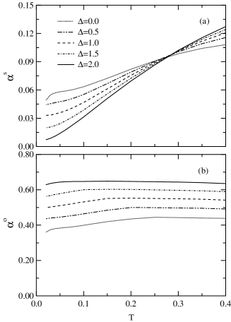
FIG. 1.: Temperature dependences of (a) $\alpha^{\rm s}$ and (b) $\alpha^{\rm o}$ for each value of $\Delta$.

In order to investigate the dynamical properties of the spin and orbital fluctuations, we define local spin and orbital susceptibilities as

$${\rm Im}\chi^{\rm s(o)}_{\mu\nu,mn}(\omega)=\frac{1}{N_{0}}\sum_{\bf q}{\rm Im}\chi^{\rm s(o)}_{\mu\nu,mn}({\bf q},\omega+{\rm i}\delta),$$ (73)

where $\delta$ is a positive infinitesimal quantity. The analytical continuation of $\chi^{\rm s(o)}_{\mu\nu,mn}(q)$ to the real axis is carried out by the Pad$\acute{\rm e}$ approximants. In order to clarify contributions to the longitudinal and transverse components of the orbital fluctuation from ${\rm Im}\chi^{\rm o}_{\mu\nu,mn}(\omega)$, we introduce operators of the charge density, longitudinal orbital density, and transverse orbital density as $\rho_{\bf i}=(1/2)\sum_{m,\sigma}f_{{\bf i}m\sigma}^{{\dagger}}f_{{\bf i}m\sigma}$, $\tau_{\bf i}^{L}=(1/2)\sum_{m,n,\sigma}f_{{\bf i}m\sigma}^{{\dagger}}\tau^{z}_{mn}f_{{\bf i}n\sigma}$, and $\tau_{\bf i}^{T}=\sum_{m,n,\sigma}f_{{\bf i}m\sigma}^{{\dagger}}(\hat{\tau}^{x}+{\rm i}\hat{\tau}^{y})_{mn}f_{{\bf i}n\sigma}$, respectively. Dynamical susceptibilities for these operators are defined as

$$\chi^{\rm o}_{\rm C}(\omega)={\rm i}\int^{\infty}_{0}dt\hskip 2.84526pte^{{\rm i}\omega t-\delta t}\langle[\rho_{\bf i}(t),\rho_{\bf i}(0)]\rangle,$$ (74)

$$\chi^{\rm o}_{\rm L}(\omega)={\rm i}\int^{\infty}_{0}dt\hskip 2.84526pte^{{\rm i}\omega t-\delta t}\langle[\tau_{\bf i}^{L}(t),\tau_{\bf i}^{L}(0)]\rangle,$$ (75)

$$\chi^{\rm o}_{\rm T}(\omega)={\rm i}\int^{\infty}_{0}dt\hskip 2.84526pte^{{\rm i}\omega t-\delta t}\langle[\tau_{\bf i}^{T}(t),\tau_{\bf i}^{T}(0)]\rangle,$$ (76)

where these quantities correspond to the local components of the net charge fluctuation, the longitudinal orbital fluctuation, and the transverse orbital fluctuation, respectively. By using $\chi^{\rm o}_{\mu\nu,mn}(\omega)$, these dynamical susceptibilities are described as

$$\chi^{\rm o}_{\rm C}(\omega)=\frac{1}{2}[\chi^{\rm o}_{11,11}(\omega)+\chi^{\rm o}_{22,22}(\omega)+2\chi^{\rm o}_{11,22}(\omega)],$$ (77)

$$\chi^{\rm o}_{\rm L}(\omega)=\frac{1}{2}[\chi^{\rm o}_{11,11}(\omega)+\chi^{\rm o}_{22,22}(\omega)-2\chi^{\rm o}_{11,22}(\omega)],$$ (78)

$$\chi^{\rm o}_{\rm T}(\omega)=\chi^{\rm o}_{21,21}(\omega),$$ (79)

where we make use of relation $\chi^{\rm o}_{11,22}(\omega)=\chi^{\rm o}_{22,11}(\omega)$. The frequency dependence of ${\rm Im}\chi^{\rm s}_{\mu\nu,mn}(\omega)$ (${\rm Im}\chi^{\rm o}_{\rm X}(\omega)$) for $\Delta/t=0$ and $\Delta/t=2$ are shown in Fig. 2(a) and Fig. 2(b) (in Fig. 2(c) and Fig. 2(d)), respectively. From these figures, one can see that the intensity of ${\rm Im}\chi^{\rm s}_{11,11}(\omega)$ in low-energy region develops with increasing $\Delta$ while intensities of two components of the orbital fluctuations are suppressed and net charge fluctuation almost unchanged. In the present case, it is understood that the spin fluctuation of the $f$-electron belonging to $\tau$=1 orbital (corresponding to $\Gamma_{8}^{(1)}$) provides predominant contribution compared with other fluctuations. The longitudinal orbital fluctuation seems to play the secondary role.

Here we comment on the reason why intensities of the orbital fluctuations in the low-energy region do not develop significantly even for the case of $\Delta$=0. We note that any spectral functions satisfy the sum rule in the frequency space. It means that suppression of the spectrum in the low-energy region leads to enhancement of that in the high-energy region or vice versa. In the present Hamiltonian, the $f$-electron number in the $\tau$=1 orbital $n_{1}$ is larger than $n_{2}$ due to the difference of the strength of hopping integrals included in the kinetic term $\epsilon_{{\bf k}11}$ and $\epsilon_{{\bf k}22}$. Since $n_{1}-n_{2}\neq 0$ in this case, the orbital polarization represented by $\tau_{\bf i}^{L}$ is non-zero, the longitudinal orbital fluctuation should be suppressed by the factor of $\langle\tau_{\bf i}^{L}\rangle^{2}$. This is the reason why the spectrum of the longitudinal orbital fluctuation in the low-energy region is suppressed even for the case of $\Delta$=0.

In order to discuss the nature of transverse orbital fluctuation, we derive the asymptotic forms of $\chi^{\rm s(o)}_{\mu\nu,mn}({\bf q},z)$ for $z\gg 1$ as

$$\chi^{\rm s(o)}_{\mu\nu,mn}({\bf q},z)\approx-\delta\chi^{\rm s(o)}_{\mu\nu,mn}({\bf q})\frac{1}{z}+O(\frac{1}{z^{2}}),$$ (80)

with coefficients

$$\delta\chi^{\rm s(o)}_{12,12}({\bf q})=-\delta\chi^{\rm s(o)}_{21,21}({\bf q})=\frac{1}{2}(n_{1}-n_{2}),$$ (81)

for ($\mu\nu,mn$)=(12,12) or (21,21) and

$$\delta\chi^{\rm s(o)}_{\mu\nu,mn}({\bf q})=0$$ (82)

for other cases. Note that $\chi^{\rm o}_{21,21}({\bf q},z)$ is just equal to $\chi^{\rm o}_{\rm T}({\bf q},z)$. From these expressions, we can conclude that in the present case of $n_{1}-n_{2}\neq 0$, the intensity of spectrum for the transverse orbital fluctuation shifts to higher energy region to satisfy the sum rule. Thus, the significant difference of the $f$-electron numbers for the two orbitals prevents essential development of the low-energy excitation for the orbital fluctuations. By noting that the value of $n_{1}-n_{2}$ is controlled by the orbital splitting energy $\Delta$ included in $\epsilon_{{\bf k}11}$ and $\epsilon_{{\bf k}22}$, it is considered that not only the longitudinal orbital fluctuation but also the transverse orbital fluctuation are suppressed by increasing the orbital splitting energy.

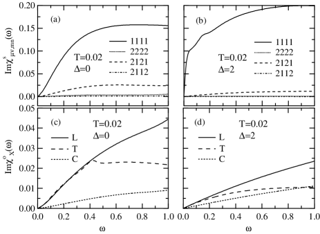
FIG. 2.: Spectra of the local components of (a) spin and (c) orbital susceptibilities for $\Delta$=0. (b) and (d) are for $\Delta$=2. For (a) and (b), solid, dotted, dashed, and dash-dotted lines describe components of $\mu\nu mn$=1111, 2222, 2121, and 2112, respectively. For (c) and (d), solid, dashed, and dotted lines correspond to X=L, T, and C, respectively.

The momentum, ${\bf q}$, dependences of the principal components of $\hat{\chi}^{\rm s}({\bf q},0)$ and $\hat{\chi}^{\rm o}({\bf q},0)$ are shown in Fig. 3, at a fixed temperature $T$=0.02 for different orbital splitting energy, $\Delta$. The upper and lower panels indicate the results for $\Delta$=0 and $\Delta$=2, respectively. For $\Delta$=0, the antiferromagnetic spin fluctuation in the $\tau$=1 orbital corresponding to $\Gamma_{8}^{(1)}$ is enhanced, but not sufficiently developed to induce $d_{x^{2}-y^{2}}$-wave superconductivity. With increasing the orbital splitting energy to $\Delta$=2, the antiferromagnetic spin fluctuation for the $\tau$=1 orbital further develops, and orbital fluctuations are completely suppressed compared with the well developed antiferromagnetic spin fluctuation.

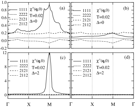
FIG. 3.: q-dependences of (a) spin and (b) orbital susceptibilities for $\Delta$=0. (c) and (d) are for $\Delta$=2. For all figures, solid, dotted, dashed, and dash-dotted lines describe components of $\mu\nu mn$=1111, 2222, 2121, and 2112, respectively.

Let us compare the present results shown in Fig. 3 with those obtained within the RPA in the previous work. [20] For $\Delta$=0, the antiferromagnetic spin fluctuation in the $\tau$=1 orbital already develops without increasing $\Delta$, while similar momentum dependences for many components of the spin and orbital susceptibilities has been seen within the RPA. When the orbital splitting energy is increased, the antiferromagnetic spin fluctuation in the $\tau$=1 orbital obtained within the FLEX approximation is considerably enhanced in comparison with that within the RPA. The considerable development of the antiferromagnetic spin fluctuation may rather prevent $d_{x^{2}-y^{2}}$-wave superconductivity because of decoupling effect through the fluctuation exchange self-energy.

B Phase Diagram

In Fig. 4, the phase diagram obtained within the FLEX approximation for the orbital degenerate system is shown, where the solid and open circles describe the superconducting and antiferromagnetic transition points, respectively. Although we do not carry out the FLEX calculation in the broken symmetry states, we may expect that the first-order phase transition between the $d_{x^{2}-y^{2}}$-wave superconducting phase and the antiferromagnetic phase takes place in the quasi-two dimensional system as discussed for the three-dimensional Hubbard model. [22] For the latter case, it has been shown that the increase of the three-dimensionality expands (shrinks) the magnetic ($d_{x^{2}-y^{2}}$-wave superconducting) phase and the coexistent phase between the $d_{x^{2}-y^{2}}$-wave superconducting and magnetic phases appears only for the system having the moderate three-dimensionality. From this consideration, the dotted curve is drawn as the first-order phase boundary expected between the two phases.

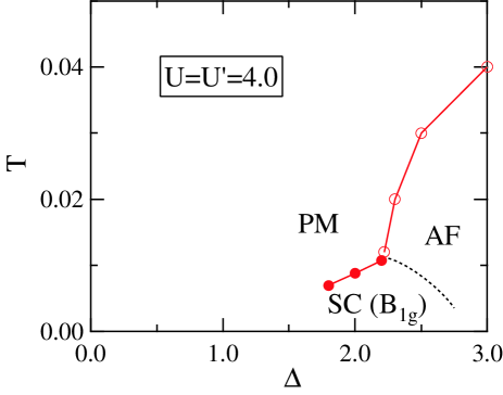
FIG. 4.: Phase diagram in the $T$-$\Delta$ plane for $U$=$U^{\prime}$=4.0 obtained by the FLEX approximation. The dotted curve is drawn by hand as expected phase boundary of first-order phase transition between the $d_{x^{2}-y^{2}}$-wave superconducting phase and the antiferromagnetic phase. In the figure, PM, AF, and SC(B_1g) express paramagnetic, antiferromagnetic, and $d_{x^{2}-y^{2}}$-wave superconducting phases, respectively.

From Fig. 4, we see that (1) the spin-singlet superconducting phase with $B_{\rm 1g}$-symmetry appears next to the antiferromagnetic phase and (2) $T_{\rm c}$ is enhanced with increasing the orbital splitting energy $\Delta$. Recalling the expression of the effective pairing interaction for spin-singlet state $T^{\rm s}_{\mu m,n\nu}(q)$, the increase of $T_{\rm c}$ with increasing $\Delta$ is ascribed to the development of the antiferromagnetic spin fluctuation and the suppression of the orbital fluctuation, where the spin and orbital fluctuations are destructive each other for the spin-singlet pair. From these observations, we conclude that the superconducting phase is induced by the development of the antiferromagnetic spin fluctuation for the $\tau$=1 orbital accompanied by suppression of the orbital fluctuation with increasing the orbital splitting energy $\Delta$.

V Discusion and Summary

Based on the simple model with orbital degree of freedom, we have shown that in the system of the density of one electron per site, the $d_{x^{2}-y^{2}}$-wave superconducting transition temperature becomes higher for the larger orbital splitting energy. For sufficiently large orbital splitting energy, the antiferromagnetic transition takes place at a N$\acute{e}$el temperature. Here we discuss the experimental results for CeTIn₅ from the present theoretical results. Analyses of experimental data of magnetic susceptibilities by using the CEF theory have determined the level schemes of CeTIn₅ compounds where the two $\Gamma_{7}$ are lower than the $\Gamma_{6}$. [15, 16] The energy splitting between the two $\Gamma_{7}$ is estimated as 68K for CeRhIn₅, 61K for CeIrIn₅, and 151K for CeCoIn₅. As we have mentioned in introducing the present model, we focus on these orbital splitting energies of the compounds regardless of kind of excited Kramers doublet. Considering that the effect of the orbital degree of freedom is generally quenched by increasing the orbital splitting energy, the present result may be independent of details of level scheme in orbital degenerate models. Namely, the present result seems to be consistent with the experimental one in the sense that $T_{\rm c}$ in CeCoIn₅ with larger orbital splitting energy is higher than that in CeIrIn₅. Thus, one can expect that the orbital splitting energy actually plays a role of controlling parameter for the superconductivity around the antiferromagnetic phase in the heavy fermion system of CeTIn₅ compounds.

On the other hand, the present theory seems to be inadequate to explain the antiferromagnetism of CeRhIn₅ with the level scheme similar to CeIrIn₅. Recent de Haas-van Alphen experiment of CeRhIn₅ has reported that the Fermi surfaces are almost unchanged up to 2.1 GPa slightly higher than the critical pressure at which the curves of the superconducting and antiferromagnetic boundaries cross each other. [23] This may mean that the $f$-electronic states are much lower than the Fermi level, and local character of $f$-electron is dominant in this compound. Thus, it will be a future problem to clarify the antiferromagnetism of CeRhIn₅ by developomg a microscopic theory based on the local property of $f$-electrons.

It is instructive to recall that the present Hamiltonian with considerably large $\Delta$ in the quarter-filling is regarded as an effective Hamiltonian in the hole-picture for the CuO₂ plane of the cuprate La₂CuO₄ which is the parent compound of high-$T_{\rm c}$ cuprate where $d_{x^{2}-y^{2}}$- and $d_{3z^{2}-r^{2}}$-orbitals just correspond to $\Gamma_{8}^{(1)}$ and $\Gamma_{8}^{(2)}$ in the present model, respectively. Considering this similarity, it may be a reasonable speculation that a superconducting phase may appear next to the antiferromagnetic phase of La₂CuO₄ in some situation where distance between the apical O- and the planer Cu-sites is shrunk, the orbital splitting energy between $d_{x^{2}-y^{2}}$- and $d_{3z^{2}-r^{2}}$-orbitals is decreased, after all.

In summary, based on the effective microscopic model with orbital degeneracy for $f$-electron systems, we have developed the strong-coupling theory for superconductivity. Considering the time reversal symmetry involved in the model, one can show that the orbital antisymmetric component of gap function hardly contributes to superconductivity because of the odd-frequency dependence. Using the FLEX approximation in which the spectra of $f$-electrons, the spin and orbital fluctuations, and the superconducting gap functions are determined consistently, it has been shown that the $d_{x^{2}-y^{2}}$-wave superconducting phase is induced by increasing the orbital splitting energy which leads to the development and suppression of the spin and orbital fluctuations, respectively. Based on these results, we have proposed that the orbital splitting energy is the key parameter controlling the changes from the paramagnetic to the antiferromagnetic phases with the $d_{x^{2}-y^{2}}$-wave superconducting phase in between.

REFERENCES

- [1] C. Petrovic, R. Movshovich, M. Jaime, P. G. Pagliuso, M. F. Hundley, J. L. Sarrao, Z. Fisk, and J. D. Thompson, Europhys. Lett. 53, 354 (2001).
- [2] C. Petrovic, P. G. Pagliuso, M. F. Hundley, R. Movshovich, J. L. Sarrao, J. D. Thompson, Z. Fisk, and P. Monthoux, J. Phys.: Condens. Matter 13, L337 (2001).
- [3] H. Hegger, C. Petrovic, E. G. Moshopoulou, M. F. Hundley, J. L. Sarrao, Z. Fisk, and J. D. Thompson, Phys. Rev. Lett. 84, 4986 (2000).
- [4] Y. Haga, Y. Inada, H. Harima, K. Oikawa, M. Murakawa, H. Nakawaki, Y. Tokiwa, D. Aoki, H. Shishido, S. Ikeda, N. Watanabe, and Y. nuki, Phys. Rev. B63, 060503(R) (2001).
- [5] R. Settai, H. Shishido, S. Ikeda, Y. Murakawa, M. Nakashima, D. Aoki, Y. Haga, H. Harima, and Y. nuki, J. Phys.: Condens. Matter. 13 L627 (2001).
- [6] Y. Kohori, Y. Yamato, Y. Iwamoto, and T. Kohara, Eur. Phys. J. B18, 601 (2000).
- [7] G.-q. Zheng, K. Tanabe, T. Mito, S. Kawasaki, Y. Kitaoka, D. Aoki, Y. Haga, and Y. nuki, Phys. Rev. Lett. 86, 4664 (2001).
- [8] K. Izawa, H. Yamaguchi, Yuji Matsuda, H. Shishido, R. Settai, and Y. nuki, Phys. Rev. Lett. 87, 057002 (2001).
- [9] P. G. Pagliuso, C. Petrovic, R. Movshovich, D. Hall, M. F. Hundley, J. L. Sarrao, J. D. Thompson, and Z. Fisk, Phys. Rev. B64, R100503 (2001).
- [10] T. Maehira, T. Hotta, K. Ueda, and A. Hasegawa, J. Phys. Soc. Jpn. 72, 854 (2003) and see also J. Phys. Soc. Jpn. Suppl. A 71, 285 (2002).
- [11] D. J. Scalapino, Phys. Rep. 250, 329 (1995).
- [12] T. Moriya and K. Ueda, Adv. Phys. 49, 555 (2000).
- [13] M. Sigrist and K. Ueda, Rev. Mod. Phys. 63, 239 (1991).
- [14] N. E. Bickers, D. J. Scalapino, and S. R. White, Phys. Rev. Lett. 62, 961 (1989) and see also N. E. Bickers and D. J. Scalapino, Ann. Phys. (N.Y.)193, 206 (1989).
- [15] T. Takeuchi, T. Inoue, K. Sugiyama, D. Aoki, Y. Tokiwa, Y. Haga, K. Kindo, and Y. nuki J. Phys. Soc. Jpn. 70, 877 (2001).
- [16] H. Shishido, R. Settai, D. Aoki, S. Ikeda, H. Nakawaki, N. Nakamura, T. Iizuka, Y. Inada, K. Sugiyama, T. Takeuchi, K. Kindo, T. C. Kobayashi, Y. Haga, H. Harima, Y. Aoki, T. Namiki, H. Sato, and Y. nuki J. Phys. Soc. Jpn. 71, 162 (2002).
- [17] Although orbital ordering states are affected by kind of excited Kramers doublet, such states are not considered in this paper.
- [18] T. Hotta and K. Ueda, Phys. Rev. B67, 104518 (2003).
- [19] Note that the hopping matrices for electrons are identical with those for -electrons where and orbitals correspond to and in this model, respectively. See, for instance, E. Dagotto, T. Hotta, and A. Moreo, Phys. Rep. 344, 1 (2001).
- [20] T. Takimoto, T. Hotta, T. Maehira, and K. Ueda, J. Phys.: Condens. Matter. 14 L369 (2002). For the case of orbitals, see T. Takimoto, Phys. Rev. B62, R14641 (2000).
- [21] J. J. Deisz, D. W. Hess, and J. W. Serene, Recent Progress in Many-Body Theories, edited by E. Schachinger et al. (Plenum Press, New York, 1995), Vol. 4.
- [22] T. Takimoto and T. Moriya, Phys. Rev. B66, 134516 (2002).
- [23] H. Shishido, R. Settai, S. Araki, T. Ueda, Y. Inada, T. C. Kobayashi, T. Muramatsu, Y. Haga, H. Harima, and Y. nuki Phys. Rev. B66, 214510 (2002).