Measuring geometric phases of scattering states in nanoscale electronic devices

Abstract

We show how a new quantum property, a geometric phase, associated with scattering states can be exhibited in nanoscale electronic devices. We propose an experiment to use interference to directly measure the effect of the new geometric phase. The setup involves a double path interferometer, adapted from that used to measure the phase evolution of electrons as they traverse a quantum dot (QD). Gate voltages on the QD could be varied cyclically and adiabatically, in a manner similar to that used to observe quantum adiabatic charge pumping. The interference due to the geometric phase results in oscillations in the current collected in the drain when a small bias across the device is applied. We illustrate the effect with examples of geometric phases resulting from both Abelian and non-Abelian gauge potentials.

Nanoscale electronic devices can exhibit distinct quantum features such as interference schuster ; ji , entanglement bena , discrete charge kastner , the Aharonov-Bohm effect yacoby , and Berry’s phase berry . The effect of Berry’s phases associated with both Abelian and non-Abelian gauge potentials has found possible applications in quantum computation jones ; zanardi . In systems with discrete energy levels, Berry’s phase makes use of the adiabatic theorem schiff and requires that the frequency of variation of parameters be much less than the energy level spacing. Berry’s phase has been demonstrated in a variety of microscopic sw89 as well as mesoscopic systems fazio .

A natural question arises as to whether or not there is a geometric phase accompanying a scattering state in a cyclic and adiabatic variation of external parameters which characterize an open system with a continuous energy spectrum. An important example of such scattering states are those present in a nanoscale electronic device coupled to electrical leads. This question has been addressed recently in the context of quantum adiabatic pumping of charge and spin in nanoscale electronic devices zhou1 . The latter is subject to intense study b98 , motivated by the experimental realization reported in the works of Marcus and co-workers switkes ; marcus . It was found that quantum adiabatic scattering provides another setting in which both Abelian and non-Abelian gauge potentials arise naturally. It was noticed that two gauge potentials may be defined in terms of the row and column vectors of instantaneous (frozen) scattering matrix, respectively. They are connected with each other via a time-reversal operation. Indeed, the scattering states associated with Hamiltonian accumulate geometric phases defined by the row vectors whereas the scattering states associated with the time-reversed Hamiltonian accumulate geometric phases defined by the column vectors. The connection between the geometric phases for the time-reversed scattering states and quantum adiabatic pumping was clarified in Ref.zhou1 . In fact, the same non-Abelian gauge field as that found by Moody et al. msw86 for a diatomic molecule also appears in an open system describing the tunneling from a scanning tunneling microscopic tip through a single magnetic spin zhou1 . However, it remains open how to experimentally observe the geometric phase for a scattering state itself.

In this Letter, we describe the general theory characterizing geometric phases for scattering states associated to a Hamiltonian with a continuous energy spectrum. A possible experimental setup utilizing nanoscale electronic devices is proposed to directly measure the effect of the geometric phases in an interference experiment. The experimental setup is similar to that used to measure the phase evolution of electrons as they traverse a QD, with some adaptation to accommodate the adiabatic variation of external parameters, e.g., gate voltages. It turns out that the geometric phase manifests itself in oscillations in the current collected in the drain when a small bias across the device is applied.

Consider an open quantum mechanical system characterized by the Hamiltonian $H(t)$ with a continuous energy spectrum, which undergoes an adiabatic evolution. By “adiabatic” we mean that the time particles “dwell” inside the scattering region is much shorter than the adiabatic period. Then the system is well described by the frozen instantaneous scattering matrix $S(t)$ thirring ; avron , which is a $2N\times 2N$ matrix, with $N$ the number of channels (such as spin) for the incoming and outgoing waves. Define vectors ${\mathbf{n}}_{\alpha}=(S_{\alpha 1},\cdots,S_{\alpha,2N})(\alpha=1,\cdots,N)$ in terms of the rows of the scattering matrix. These vectors are orthonormal and so constitutes a smooth set of local bases. As the system undergoes an adiabatic and cyclic evolution and returns to the initial configuration, the interplay between the adiabatic (dynamic) evolution and the global geometric property implies that the row vectors ${\bf n}_{\alpha}$ acquire a geometric phase,

$$U={\rm P}\exp(i\oint\sum_{\nu}A_{\nu}dV_{\nu}),$$ (1)

where P denotes path ordering, $A_{\alpha\beta\nu}=i\;{\bf n}^{*}_{\beta}\cdot\partial_{\nu}{\bf n}_{\alpha}$ ($\partial_{\nu}\equiv\partial/\partial V_{\nu}$) is the gauge potential, and $V_{\nu}$ are independent slowly varying external parameters. Here we emphasize that, unlike Berry’s phases, the causality condition plays an essential role, which states that scattered waves appear only after the incident wave hits the scatterer. Under the gauge transformation which mixes up scattering states from different channels ${\bf n}^{\prime}_{\alpha}=\sum_{\beta}\omega_{\alpha\beta}{\bf n}_{\beta}$, the gauge potential defined by $A=\sum_{\nu}A_{\nu}dV_{\nu}$ transforms as

$$A^{\prime}=id\omega\omega^{-1}+\omega A\omega^{-1}.$$ (2)

That is, $A$ describes $U(N)$ gauge potentials arising from the superposition of different channel scattering states. As a special case, the Abelian gauge group $U(1)$ originates from the fact that the absolute phase is not observable in quantum mechanics. The adiabatic variation of the scattering potential $V(x,t)$ induces a local gauge transformation ${\bf n}^{\prime}=\exp(i\varphi){\bf n}$ due to the time dependence of the phase $\varphi$ in quantum mechanics.

Let us now turn to a specific proposal as to how to experimentally observe the effect of the geometric phase, in a mesoscopic electronic device. We emphasize that the theory presented here is not restricted to mesoscopic physics, but to any system described by scattering states with continuous energy spectrum. We also emphasize that, although (for reasons of concreteness) we consider a specific potential for a quantum dot, the general idea applies to scattering states in general. Consider a QD modeled by a potential $V(x)$ with $x$ denoting the coordinate (see Fig. 1A). For reasons of simplicity, we choose the potential $V(x)$ as $0$ for $|x|\geq a$, $V_{1}$ for $-a<x<-b$, $V_{2}$ for $|x|\leq b$, and $V_{3}$ for $b<x<a$. For a QD of size 800 nm (see Fig. 1), the energy level spacing is of the order of 4.5 meV. The Coulomb energy, assuming a dielectric constant of 10, is of the order of 0.08 meV. Thus, the dimension of the QD is such that the Coulomb energy is much less than the separation between the resonances and can be ignored. Also the spin-dependent scattering inside the QD is ignored. Then the instantaneous $2\times 2$ scattering matrix $S(t)$ for the QD is determined from the solution of the Schrödinger equation $(-(\hbar^{2}/2m)\partial^{2}/\partial x^{2}+V(x)-E)\psi=0$. Let $r_{QD}$ and $t_{QD}$ denote, respectively, the reflection and transmission coefficients of the QD for the left incident electron, and $r^{\prime}_{QD}$ and $t^{\prime}_{QD}$ denote, respectively, the reflection and transmission coefficients of the QD for the right incident electron, which are functions of the parameters of the QD. If the potential is mirror symmetric, i.e., $V_{1}=V_{3}$, then $t_{QD}=t^{\prime}_{QD}$ and $r_{QD}=r^{\prime}_{QD}$ and the geometric phase is trivial. Therefore, to observe a nontrivial geometric phase it is necessary to break the mirror symmetry of the potential. This implies that we have to choose $V_{1}\neq V_{3}$.

Suppose we periodically and adiabatically vary independent external parameters $V_{1}$, $V_{2}$, and $V_{3}$. For instance, we can choose to adiabatically change $V_{1}$ and $V_{2}$ with $V_{3}$ kept constant, i.e., $V_{1}=V^{0}_{1}+\Delta V_{1}\sin\Omega t,~{}V_{2}=V^{0}_{2}+\Delta V_{2}[\sin(\delta+\Omega t)-\sin\delta],V_{3}=V^{0}_{3},~{}(\Delta V_{1,2}\ll V^{0}_{1,2})$, with $\Omega$ being the slow frequency characterizing the adiabaticity and $\delta$ the phase difference. (The presence of an extra term $-\Delta V_{2}\sin\delta$ is only to ensure that the initial state is the same for all different contours.) In our case, this may be achieved by controlling the gate voltages such that the dwell time $\tau_{d}$ during which electrons scatter off the QD is much shorter than the period $T=2\pi/\Omega$ during which the system completes the whole adiabatic cyclic process. In such a limit, electrons well-defined in the incident energy $E$ are scattered at a well-defined time $t$ as measured at large time scale by the adiabatic cycle period $T$, consistent with the Heisenberg uncertainty principle. That is, it makes sense to speak of the instantaneous scattering matrix for electrons with a given incident energy. Then, in addition to the dynamic phase, the scattered waves accumulate a geometric phase factor $e^{i\gamma}$ during one cycle with $\gamma$ given using Eq.(1) for the $U(1)$ case. Now ${\bf n}$ denotes the row vector of the scattering matrix $S$, i.e., ${\bf n}=(r_{QD},t_{QD})$, so that

$$\gamma=\oint r^{*}_{QD}dr_{QD}+t_{QD}^{*}dt_{QD}=\oint A_{1}dV_{1}+A_{2}dV_{2}+A_{3}dV_{3},$$ (3)

since $r_{QD}$ and $t_{QD}$ depend on any variables which vary during the cycle. Here we assume all $V$’s are changing with time. However, if any of them is kept constant the corresponding term disappear. In this case, the gauge transformation, Eq.(2), becomes

$$A^{\prime}=A-d\varphi.$$ (4)

The curvature defined by $dA$ is gauge invariant, which allows us to rewrite $\gamma$ in the form $\gamma=\iint dA$ using Stokes’ theorem, where the integral is over the area encircled by the contour. This implies the gauge invariance of the geometric phase. For the specific case when the variation is very small $\gamma$ is simply proportional to the area swept out in the parameter space. The geometric phase is plotted in Fig. 1B as a function of $\Delta V_{1}$, with $\Delta V_{2}=0$, $\Delta V_{3}$ kept constant at $V^{0}_{3}/10$, and $\delta=\pi/2$. As we see, $\gamma$ behaves linearly as $\Delta V_{1}$ changes, resulting from the fact that energy-dependent resonances on the QD are robust for the variation of $V_{1}$. However, the slope sensitively depends on whether we are on or off resonance. Similarly, we plot the phase $\gamma$ in Figs. 1C and 1D as a function of $\Delta V_{2}$ when $\Delta V_{1}$ is kept constant at $V^{0}_{1}/10$ and $\Delta V_{3}=0$, with the incident energy $E$ being off and on a resonance at the initial state, respectively. The oscillating behavior indicates that $\gamma$ is quite sensitive to the presence of the resonant levels inside the contour in the parameter space $\{V_{1},V_{2}\}$, as displayed in the insets in Figs. 1B-D. A jump occurs in the geometric phase if the contour encircles a new transmission resonance.

Having described how the geometric phase appears for the scattering state using a QD, we now consider how to measure it experimentally. The experimental setup we propose is the double path interferometer (see Fig. 1A), which previously was used to measure the phase evolution of electrons as they traverse a QD ji ; schuster . The measurement proceeds as follows. The system is prepared in some scattering state with incident energy $E$ for certain initial values of the external parameters $V_{1}$, $V_{2}$ and $V_{3}$, which are controllable by adjusting the Fermi level in the leads and the attached gate voltages, respectively. Then, the gate voltages are varied in a cyclic manner and sufficiently slowly that the system always remains in the instantaneous scattering state at any later instant $t$. Electrons in the reference path and QD-path interfere and is observed as oscillations in the current collected in the drain in the linear response regime, i.e., in the presence of a small bias across the QD. A crucial feature of the device here, in contrast to the experimental setups used to observe adiabatic pumping currents switkes , is that the reflected electrons are allowed to escape from the interferometer between the source and the drain, thus violating current conservation. This prevents multiple scattering processes which dominate quantum adiabatic pumping as current conservation requires. It is this feature that makes it possible to capture the effect of the geometric phases for scattering states.

The device we suggested above involves quantum interferometry of geometric phases in a mesoscopic open system. This is similar to the Aharonov-Bohm effect, which leads to an oscillating periodic component in the current as a function of magnetic field applied ji ; schuster ; yacoby . However, instead of the flux produced by the external magnetic field, here the geometric phase results from the gauge field induced by the adiabatic dynamics of the QD. The total device transmission ${\cal T}$ resulting from the two-path interference after one period $T$ takes the form

$${\cal T}=|t_{ref}|^{2}+|t_{QD}|^{2}+2|t_{ref}||t_{QD}|\cos(\gamma+\varphi_{12}).$$ (5)

Here $t_{ref}$ denotes the transmission coefficient for the reference path, and $\varphi_{12}$ is the phase difference between the two transmission coefficients $t_{ref}$ and $t_{QD}$, which only depends on the initial scattering state. In fact, Eq.(5) is gauge invariant, as it should be, and holds at any instant $t$ as long as $t_{ref},t_{QD}$ and $\gamma$ take the instantaneous values, because the transmission ${\cal T}$ describes the current collected in the drain and so is observable. However, we emphasize that only for the whole period $T$, is $\gamma$ gauge invariant and therefore observable. One may recognize that the transmission ${\cal T}$ in Eq.(5) takes the same form as that at the initial instant, except for the involvement of the geometric phase $\gamma$ in the last term. Indeed, the first and second terms just provide a background solely determined by the initial state, i.e., it does not depend on which adiabatic cycle we choose. This is in contrast to the geometric phase $\gamma$ which does depend on contours the system traverses in the parameter space. $\varphi_{12}$ also changes during the cycle, but is periodic in $T$. For different choices of the phase difference $\delta$ corresponding to different shapes of the adiabatic cycles, the transmission ${\cal T}$ varies considerably in the entire energy range. ¿From the experimental data for the interferometer reported by Schuster et al. schuster , one may estimate that the background term $|t_{ref}|^{2}+|t_{QD}|^{2}$ is approximately $1.05$ and the oscillating amplitude $2|t_{ref}||t_{QD}|$ is approximately $0.05$. Hence, for such a device the deviation coming from the presence of $\gamma$ would be approximately $0.1$. Thus, even at a relatively low visibility the effect from the scattering geometric phase should be observable. Fig. 1 and Eq.(5) imply that the effect of the geometric phase $\gamma$ on the transmission ${\cal T}$ is observable. An important issue is that the dwell time $\tau_{d}$ is longer when the QD is on resonance, so the frequency of the adiabatic variation, $\Omega$, should be sufficiently slow to ensure the adiabaticity parameter $\epsilon\equiv\Omega\tau_{d}$ to be very small. We believe that current technology is sufficient to control the adiabatic dynamics to observe the effect of the geometric phase.

Now we explain how to modify the interference setup to observe the geometric phase associated with the true non-Abelian gauge field which occurs in the context of adiabatic spin pumping. The geometric (matrix) phase $U$, from Eq.(1), is a $2\times 2$ matrix and results from the true non-Abelian gauge potential, which is the time-reversed counterpart of that studied in quantum spin pumping zhou1 . Adopting the same notations as those there, one sees that the non-Abelian gauge potential takes the same form as Eq.(8) in Ref. zhou1 , with $\phi$ replaced by $-\phi$. For a contour when $\phi$ varies from 0 to $2\pi$ with some fixed $\theta$, we have $U=\exp\{i\pi[1-\cos(\delta_{1}-\delta_{2})]\sin^{2}\theta\sigma^{3}/2\}$. In this case, the non-Abelian character of the potential is lost zee . To observe the effect of the non-Abelian gauge field, it is necessary to choose a contour which varies both $\theta$ and $\phi$. The noncommutativity of the matrix form of the gauge potential presents some difficulties to explicitly calculate the (matrix) phase $U$. However, one may use the non-Abelian version of Stokes’ theorem bralic to evaluate $U$. Alternatively, in numerical calculations, we can perform a straightforward expansion of the path ordered exponential, Eq.(1). The effect of the geometric phase is seen from the gauge invariant transmission

$${\cal T}={\rm Tr}|t_{ref}+Ut_{SI}|^{2},$$ (6)

with $t_{ref}$ and $t_{SI}$ being the $2\times 2$ transmission coefficient matrices for the reference and spin-dependent interaction paths, respectively. The interference pattern of the two paths is changed due to the geometric phase.

Note that the relative intensity of the two paths for the interferometer cannot be calculated theoretically, therefore we choose one specific value for the relative intensity. Unlike in the Abelian case, the non-Abelian geometric phase, $U$, is gauge dependent. Therefore we focus on the transmission. In Fig. 2 we plot transmission resulting from Eq.(6) as a function of $k/\Gamma$ for a contour which is a spherical rectangle. The parameters $k,J,$ and $\Gamma$ are defined in Ref. zhou1, . The solid line presents results when the geometric phase is absent. After inclusion of the geometric phase the transmission changes significantly in both amplitude and shape. Especially, the two peaks at the resonances $k/\Gamma=\pm J/\Gamma$ shift due to an energy splitting coming from the geometric phase $U$, i.e., during the adiabatic change the system moves out of resonance.

In summary, we developed a theory to describe geometric phases for scattering states, and generalized it to the spin-dependent case. We have also proposed an experimental setup to directly observe the effect from the scattering geometric phase. The effect should be large enough to be detected in an open interferometer, and observed as oscillations in the current across the device.

Figure 1: A, Proposed electronic interferometer to directly measure the geometric phase. The cyclic and adiabatic variation of the gate voltages $V_{1},V_{2}$ and $V_{3}$ pairwise imposes a geometric phase in the QD-arm. The inset shows the model one-dimensional potential inside the QD. B, Geometric phase, $\gamma$, as a function of $\Delta V_{1}$, with $\Delta V_{2}=0$, and $\Delta V_{3}$ kept constant at $V^{0}_{3}/10$. The inset shows the contours for three different values of $\Delta V_{1}$, presented as colored dots on the curve. The black dot in the inset represents the initial state. The dotted lines in the inset show the positions of transmission resonances through the QD in the parameter space for a selected incident energy $E=0.56V^{0}_{1}$, which is off resonance. C, Geometric phase, $\gamma$, as a function of $\Delta V_{2}$, with $\Delta V_{1}$ kept constant at $V^{0}_{1}/10$, and $\Delta V_{3}=0$. The inset displays the same information as in B. The geometric phase, $\gamma$, shows a dip when the contour touches a new transmission resonance. There is a significant change in $\gamma$ when $\Delta V_{2}$ varies. D, Same as c, but for a different value of the incident energy, $E$, positioned at a resonance. Parameters (in units of $V^{0}_{1},\hbar=m_{e}=1$): $a=40,b=39,V^{0}_{2}=-1.0,V^{0}_{3}-1.2,\delta=\pi/2$. (If $V_{1}^{0}\sim 60$ mV above the Fermi level and $m^{*}=0.07m_{e}$ as for GaAs, then $a\sim 410$nm, and $b\sim 400$nm.

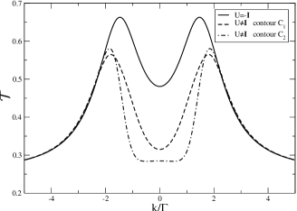
Figure 2: Total transmission through an interferometer for a non-Abelian gauge potential zhou1 , describing spin-flip scattering through a magnetic atom, calculated from Eq (6), for different choices of contours, with $J/\Gamma=1.5$. The solid line corresponds to the case when no geometric phase is present. The dashed lines gives typical results after inclusion of the geometric phase. There are two peaks at the resonances $k/\Gamma=\pm J/\Gamma$. Note that it is impossible to calculate the relative values of $t_{ref}$ and $t_{QD}$ theoretically, due to the nature of the interferometer. As a sample case we take the phase difference between $t_{ref}$ and $t_{QD}$ to be $\pi$, so that $t_{ref}=-{\mathbf{I}}$. The smaller contour chosen is $C_{1}(\theta_{1},\phi_{1},\theta_{2},\phi_{2})=[\pi/2,0,\pi/4,\pi/2]$ and the larger is $C_{2}(\theta_{1},\phi_{1},\theta_{2},\phi_{2})=[\pi/2,0,\pi/4,\pi]$ (in the same notation as Ref. zhou1 ).

- (1) R. Schuster et al., Nature 385, 420 (1997);
- (2) Y. Ji et al., Science 290, 779 (2000).
- (3) C. Bena, S. Vishveshwara, L. Balents, and M.P. Fisher, Phys. Rev. Lett. 89, 037901 (2002).
- (4) M.A. Kastner, Rev. Mod. Phys. 64, 849 (1992).
- (5) A. Yacoby, M. Heiblum, D. Mahalu, and H. Shtrikman, Phys. Rev. Lett. 74, 4047 (1995).
- (6) M.V. Berry, Proc. Roy. Soc. London, Ser. A 392, 45 (1984).
- (7) J. Jones, V. Vedral, A.K. Ekert, and C. Castagnoli, Nature 403, 869 (2000).
- (8) P. Zanardi, and M. Rasetti, Phys. Lett. A 264, 94 (1999).
- (9) L. I. Schiff, Quantum mechanics (McGraw-Hill, New York, 1955), p. 290.
- (10) Geometric Phases in Physics, edited by A. Shapere and F. Wilczek (World Scientific, Singapore, 1989).
- (11) G. Falci et al., Nature 407, 355 (2000).
- (12) H.-Q. Zhou, S.Y. Cho, and R.H. McKenzie, Phys. Rev. Lett. 91, 186803 (2003).
- (13) P.W. Brouwer, Phys. Rev. B 58, R10135 (1998); M. Büttiker, H. Thomas, and A. Prétre, Z. Phys. B 94, 133 (1994); M. Moskalets and M. Büttiker, Phys. Rev. B 66, 035306 (2002); F. Zhou, B. Spivak, and B. Altshuler, Phys. Rev. Lett. 82, 608 (1999); J.E. Avron, A. Elgart, G.M. Graf, and L. Sadun, Phys. Rev. Lett. 87, 236601 (2001); Y. Makhlin, and A.D. Mirlin, Phys. Rev. Lett. 87, 276803 (2001); A. Andreev and A. Kamenev, Phys. Rev. Lett. 85, 1294 (2000).
- (14) M. Switkes, C.M. Marcus, K. Campman, and A.C. Gossard, Science 283, 1905 (1999).
- (15) S.K. Watson, R.M. Potok, C.M. Marcus, and V. Umansky, cond-mat/0302492 (unpublished).
- (16) J. Moody, A. Shapere, and F. Wilczek, Phys. Rev. Lett. 56, 893 (1986).
- (17) H. Narnhofer and W. Thirring, Phys. Rev. A26, 3646 (1982).
- (18) J.E. Avron, A. Elgart, G.M. Graf, and L. Sadun, J. Math. Phys. 43, 3415 (2002).
- (19) A. Zee, Phys. Rev. A 38, 1 (1988).
- (20) N.E. Bralić, Phys. Rev. D 22, 3090 (1980); P. M. Fishbane, S. Gasiorowicz, and P. Kaus, Phys. Rev. D 24, 2324 (1981); L. Diósi, Phys. Rev. D 27, 2552 (1983).