A study of the static yield stress in a binary Lennard-Jones glass

Abstract

The stress-strain relations and the yield behavior of a model glass (a 80:20 binary Lennard-Jones mixtures Kob-Andersen ) is studied by means of molecular dynamics simulations. In a previous paper VBBB it was shown that, at temperatures below the glass transition temperature, $T_{\text{g}}$, the model exhibits shear banding under imposed shear. It was also suggested that this behavior is closely related to the existence of a (static) yield stress (under applied stress, the system does not flow until the stress $\sigma$ exceeds a threshold value $\sigma_{\text{y}}$). A thorough analysis of the static yield stress is presented via simulations under imposed stress. Furthermore, using steady shear simulations, the effect of physical aging, shear rate and temperature on the stress-strain relation is investigated. In particular, we find that the stress at the yield point (the “peak”-value of the stress-strain curve) exhibits a logarithmic dependence both on the imposed shear rate and on the “age” of the system in qualitative agreement with experiments on amorphous polymers Govaert ; vanAken and on metallic glasses HoHuu ; Johnson . In addition to the very observation of the yield stress which is an important feature seen in experiments on complex systems like pastes, dense colloidal suspensions DaCruz and foams Debregeas::PRL87 , further links between our model and soft glassy materials are found. An example are hysteresis loops in the system response to a varying imposed stress. Finally, we measure the static yield stress for our model and study its dependence on temperature. We find that for temperatures far below the mode coupling critical temperature of the model ($T_{\text{c}}\!=\!0.435$), $\sigma_{\text{y}}$ decreases slowly upon heating followed by a stronger decrease as $T_{\text{c}}$ is approached. We discuss the reliability of results on the static yield stress and give a criterion for its validity in terms of the time scales relevant to the problem.

I Introduction

Despite the large diversity of their microstructures, the so called soft glassy materials Sollich like pastes, dense colloidal suspensions, granular systems and foams exhibit many common rheological properties. Once in a glassy or “jammed” state, these systems do not flow, if a small shear stress is applied on them. For stresses slightly above a certain threshold value (the yield stress, $\sigma_{\text{y}}$), however, they no longer resist to the imposed stress and a flow pattern is formed Larson ; Coussot-Raynaud-et-al::PRL88::2002 ; Bonn2 ; DaCruz .

Let us illustrate this behavior using results of simulations to be described in more detail in later sections. Figure 1 shows $U_{\text{max}}$, the maximum velocity in the system measured close to the left wall during simulations of a 80:20 binary Lennard-Jones (LJ) mixture Kob-Andersen while applying a constant shear stress to the left wall (see section II for more details on the model). The applied stress is increased stepwise by an amount of $d\sigma\!=\!0.02$ every $4000$ LJ time units and $U_{\text{max}}$ is measured between two increments of the stress (note that, as seen from the inset of the same figure, this time is long enough in order to also determine the velocity profile, $u(z)$, accurately).

It is seen from Fig. 1 that, for stresses $\sigma\leq 0.6$, $U_{\text{max}}$ is hardly distinguishable from zero. In particular, it is much smaller than the thermal velocity of the wall, $U^{\text{thermal}}\!=\!\sqrt{T/M}\!\approx\!0.0236$ ($M\!=\!360$ is the mass of the wall and $T\!=\!0.2$ the temperature). Thus, at these stresses, the system remains in the jammed state and resists to the drag force transmitted to it by the left wall. However, as the stress is further increased, a remarquable change in the system mobility is observed. The system starts to flow and $U_{\text{max}}$ increases by more than two orders of magnitude.

An inspection of the corresponding velocity profiles illustrated in the inset of Fig. 1 reveals a further feature related to the yield stress, namely that, once the applied stress exceeds the yield value, the whole system fluidizes and the velocity profile is practically linear (velocity profiles corresponding to $\sigma\leq 0.6$ fluctuate around zero and are not shown in the inset).

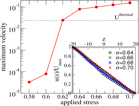
Figure 1: The maximum velocity in the system, $U_{\text{max}}$, measured in the layer of closest approach to the left wall during simulations of a binary Lennard-Jones glass [$T\!=\!0.2\;(<T_{\text{c}}\!=\!0.435)$] at imposed stress. The stress is increased by an amount of $d\sigma\!=\!0.02$ once in $4000$ LJ time units and $U_{\text{max}}$ is measured between two subsequent stress increments. The horizontal dotted line marks the thermal velocity of the wall. Note the sharp increase in $U_{\text{max}}$ when changing the stress from $\sigma\!=\!0.6$ to $0.62$. Inset: rescaled velocity profiles, $u(z)/U_{\text{max}}$, measured during the same simulations for stresses in the flow regime (for which $U_{\text{max}}\geq U^{\text{thermal}}$). Obviously, once the flow sets in, a linear velocity profile is formed across the system.

On the other hand, in experiments upon imposed shear rate, shear thinning is observed Larson ; Bonn . The apparent viscosity, defined as the average stress divided by the average overall shear rate, $\eta_{\text{app}}\!=\!\sigma/\dot{\gamma}_{\text{tot}}$, decreases with increasing $\dot{\gamma}_{\text{tot}}$ (in the case of a planar Couette-flow with wall velocity and separation $U_{\text{w}all}$ and $L_{z}$, for example, $\dot{\gamma}_{\text{tot}}\!=\!U_{\text{w}all}/L_{z}$). Furthermore, over some range of shear rates, the system separates into regions with different velocity gradients (shear bands) Bonn2 ; Coussot-Raynaud-et-al::PRL88::2002 ; Pignon::JRheo40::1996 .

Whereas the shear thinning is commonly attributed to the acceleration of the intrinsic slow dynamics by the external flow (the new time scale, $1/\dot{\gamma}_{\text{tot}}$, is much shorter than the typical structural relaxation time of the system) Sollich ; BB::PRE61::2000 ; BB2 ; Kurchan ; Lacks , the origin of the shear bands still remains to be clarified. In some cases, this shear-banding phenomenon can be understood in terms of underlying structural changes in the fluid, analogous to a first order phase transition. Examples are systems of rod like particles, entangled polymers or surfactant micelles where the constituents (rods, polymer or surfactant molecules) gradually align with increasing shear rate thus leading to a coupling between the local stress and the spatial variation of the velocity gradient olmsted ; Dhont . In the case of soft glassy materials, however, no such changes are evident, and coexistence appears between a completely steady region (zero shear rate) and a sheared, fluid region Chen ; Pignon::JRheo40::1996 ; Losert::PRL85::2000 ; Debregeas::PRL87 ; Coussot-Raynaud-et-al::PRL88::2002 .

It was shown in a previous work VBBB that a model of 80:20 binary Lennard-Jones glass Kob-Andersen also exhibits the shear banding phenomenon. Furthermore, a link was suggested between the occurence of shear bands and the existence of a static yield stress in the system. It was found that [see Fig. 2] the yield stress is larger than the steady state stress measured in a steady shear experiment in the limit of the zero shear rate, $\sigma_{\text{y}}>\lim_{\dot{\gamma}_{\text{tot}}\to 0}\sigma$. It was then suggested that, a shear-banding could be expected for shear rates, for which $\sigma(\dot{\gamma}_{\text{tot}})<\sigma_{\text{y}}$: as the flow is imposed externally (by moving, say, the left wall) the formation of a flow pattern is unavoidable. On the other hand, it follows from $\sigma(\dot{\gamma}_{\text{tot}})<\sigma_{\text{y}}$ that, some regions in the system are “rigid enough” to resist to the flow-induced stress whereas other regions undergo irreversible rearrangements more easily footnote1 . Hence, whereas the details of the “nucleation” and growth of a heterogeneous flow pattern may depend on the initial heterogeneity in the “degree of jamming” CoussotJRheh46 , “free volume” Lemaitre or “fluidity” Derec ; Picard at the beginning of the shear motion, its very origin lies in the possibility of resisting to the shear-induced stress, i.e. in the existence of a static yield stress.

Therefore, although it does not solve the problem of the selection between the two bands, the existence of a static yield stress is at least consistent with the coexistence of a jammed region and a fluidized band: once the yield stress $\sigma_{\text{y}}$ is added to the flow curve, the shear rate becomes multivalued in a range of shear stresses, a situation encountered in several complex fluids olmsted . This phenomenon should thus be generic for many soft glassy materials.

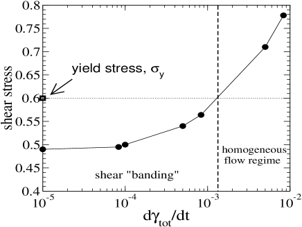
Figure 2: The shear stress versus imposed shear rate, $\dot{\gamma}_{\text{tot}}$, under homogeneous flow conditions at $T=0.2$. The square on the horizontal axis marks the yield stress measured in imposed stress simulations of a planar Couette cell [see the dramatic change in $U_{\text{max}}$ at $\sigma\!=\!0.6$ in Fig. 1, see also Fig. 17]. Under imposed shear, if the corresponding steady state stress falls below the horizontal dotted line, a heterogeneous flow can be expected, whereas in the opposite case the flow will be homogeneous. The vertical dashed line marks the shear rate on the boundary of these two flow regimes. Note that the yield stress shown here is a lower bound for $\sigma_{\text{y}}$ (see the solid line in Fig. 17) and thus is smaller than the value used in VBBB . However, as a comparison with Fig. 3 of Ref. VBBB shows, the estimated $\dot{\gamma}_{\text{tot}}$-range for heterogeneous and homogeneous flow regimes is hardly changed by this modification.

In this paper we present an extensive study of the stress-strain relations and yielding properties of the present model. The report is organized as follows. After the introduction of the model in the next section, results on the system response to an imposed overall shear rate are presented, and the effects of physical aging, shear rate and temperature on the stress-strain curves are investigated. In section IV, the response of the system to imposed stress is studied. The measurement of the static yield stress in the subject of section V. A summary compiles our results.

II Model

We performed molecular dynamics simulations of a generic glass forming system, consisting of a 80:20 binary mixture of Lennard-Jones particles (whose types we call A and B) at a total density of $\rho\!=\!\rho_{\text{A}}+\rho_{\text{B}}\!=\!1.2$. A and B particles interact via a Lennard-Jones potential, $U_{\text{LJ}}(r)\!=\!4\epsilon_{\alpha\beta}[(\sigma_{\alpha\beta}/r)^{12}-(\sigma_{\alpha\beta}/r)^{6}]$, with $\alpha,\beta\!=\!{\text{A,B}}$. The parameters $\epsilon_{\text{AA}}$, $\sigma_{\text{AA}}$ and $m_{\text{A}}$ define the units of energy, length and mass. The unit of time is then given by $\tau\!=\!\sigma_{\text{AA}}\sqrt{m_{\text{A}}/\epsilon_{\text{AA}}}$. Furthermore, we choose $\epsilon_{\text{AB}}\!=\!1.5\epsilon_{\text{AA}}$, $\epsilon_{\text{BB}}\!=\!0.5\epsilon_{\text{AA}}$, $\sigma_{\text{AB}}\!=\!0.8\sigma_{\text{AA}}$, $\sigma_{\text{BB}}\!=\!0.88\sigma_{\text{AA}}$ and $m_{\text{B}}\!=\!m_{\text{A}}$. The potential was truncated at twice the minimum position of the LJ potential, $r_{\text{c}}\!=\!2.245$. Note that the density is kept constant at the value of $1.2$ for all simulations whose results are reported here. This density is high enough so that the pressure in the system is positive at all studied temperatures. The present model system has been extensively studied in previous works BB::PRE61::2000 ; barratkob ; BB2 ; Kob-Andersen and exhibits, in the bulk state, a computer glass transition (in the sense that the relaxation time becomes larger than typical simulation times) at a temperature of $T_{\text{c}}\simeq 0.435$ Kob-Andersen . Since our aim is to study the interplay between the yield behavior and the possible flow heterogeneities, we do not impose a constant velocity gradient over the system as done in Ref. BB2 , where a homogeneous shear flow was imposed through the use of Lees-Edwards boundary conditions. Rather, we confine the system between two solid walls, which will be driven at constant velocity. By doing so, we mimic an experimental shear cell, without imposing a uniform velocity gradient.

We first equilibrate a large simulation box with periodic boundary conditions in all directions, at $T\!=\!0.5$. The system is then quenched to a temperature below $T_{\text{c}}$, where it falls out of equilibrium, in the sense that structural relaxation times are by orders of magnitude larger than the accessible simulation times. On the time scale of computer simulation, the system is in a glassy state, in which its properties slowly evolve with time towards the (unreachable) equilibrium values (aging, see Fig. 5). After a time of $t\!=\!4.10^{4}$ [$2.10^{6}$ MD steps], we create 2 parallel solid boundaries by freezing all the particles outside two parallel $xy$-planes at positions $z_{\text{wall}}\!=\!\pm L_{z}/2$ ($L_{z}\!=\!40$) [see Fig. 4]. For each computer experiment, 10 independent samples (each containing 4800 fluid particles) are prepared using this procedure. Note that the system is homogeneous in the $xy$-plane ($L_{x}\!=\!L_{y}\!=\!10$). We thus compute local quantities like the velocity profile, the temperature profile, etc. as an average over particles within thin layers parallel to the wall.

The amorphous character of our model is clearly seen by an analysis of the packing structure, i.e. the radial pair distribution function. Figure 3 shows the various kinds of radial pair distribution functions which can be defined for a binary mixture: $g_{\alpha\beta}$ is the probability (normalized to that of an ideal gas) of finding a particle of type $\alpha$ at a distance $r$ of a $\beta$-particle ($\alpha,\beta\in\{\text{A,B}\}$). In order to demonstrate that the system keeps its amorphous structure at temperatures far below the glass transition temperature of the model, we show the mentioned pair distribution functions at two characteristic temperatures, one in the supercooled state ($T\!=\!0.5>T_{\text{c}}\!=\!0.435$) and one at $T\!=\!0.2$. As seen from Fig. 3, the maxima of $g_{\alpha\beta}$ are more pronounced at lower $T$. However, no sign of crystallization or long range positional order is observed as the temperature is lowered through the glass transition.

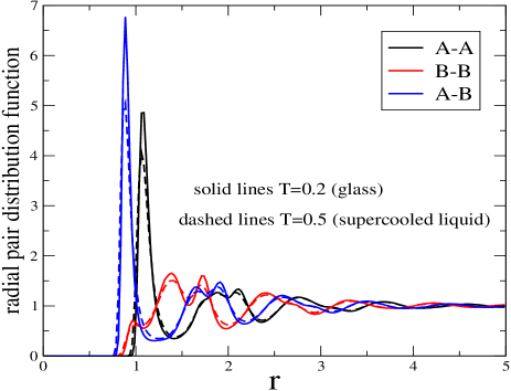
Figure 3: The radial pair distribution functions, $g_{\alpha\beta}$ ($\alpha,\beta\in\{\text{A,B}\}$) at two characteristic temperatures of $T\!=\!0.5$ (supercooled state) and $T\!=\!0.2$ (glassy state, note that the mode coupling critical temperature of the system is $T_{\text{c}}=0.435$). Note that curves belonging to $T\!=\!0.5$ and $T\!=\!0.2$ are qualitatively similar (no further peaks occur while cooling below $T_{\text{c}}$). Thus, the system maintains its liquid-like (amorphous) structure at temperatures far below $T_{\text{c}}$.

Figure 4: A snapshot of the system at a total density of $\rho=\rho_{\text{A}}+\rho_{\text{B}}=1.2$ ($\rho_{\text{A}}=0.96$ and $\rho_{\text{B}}=0.24$). The walls (darker particles) are made of the same types of particles as the fluid itself. They are distinguished from the inner particles in that either they have no thermal motion or they are coupled to equilibrium lattice sites by harmonic springs thus preventing their diffusion.

The mentioned insensitivity of the static structure to the glass transition must be contrasted to the fact that, at temperatures slightly above $T_{\text{c}}$, the system can be equilibrated within the time accessible to the simulation whereas this is no longer the case for temperatures significantly below $T_{\text{c}}$. At $T\!=\!0.5$, for example, the time necessary for an equilibration of the system is of order of a few hundred Lennard-Jones time units (not shown). For $T\!=\!0.45$, the equilibration time rises to a few thousands whereas at $T\!=\!0.2$ the system is not equilibrated even after $2\times 10^{5}$ LJ time units. At this temperature, time translation invariance does not hold and the dynamical quantities depend on two times: the actual time, $t$, and the waiting time $t_{\text{w}}$. Here, $t_{\text{w}}$ is the time elapsed after the temperature quench (from $T\!=\!0.5$ to $T\!=\!0.2$) and the beginning of the measurement.

This behavior is illustrated in Fig. 5, where the mean square displacement (MSD) of a tagged particle is shown at a temperature above $T_{\text{c}}$ ($T\!=\!0.45$) and at $T\!=\!0.2$ (far below $T_{\text{c}}$) for various waiting times. The figure nicely demonstrates the establishing of the time translation invariance (TTI) at $T\!=\!0.45$. Here, $t_{\text{w}}\!=\!0$ corresponds to a change of temperature from $T\!=\!0.5$ to $T\!=\!0.45$. As expected from the fact that $T\!=\!0.45$ belongs to the supercooled (liquid) state, with increasing waiting time, the MSD converges towards the equilibrium curve reaching it after about $4000$ Lennard-Jones time units. It is worth noting that the waiting time at which the TTI is recovered roughly corresponds to the time needed for the MSD to reach the size of a particle.

At $T\!=\!0.45$, the equilibrium curve for the MSD exhibits the well-known two step relaxation characteristic of supercooled liquid: for short times ($t\ll 1$), free particle motion with thermal velocity is observed ($[\bm{r}(t+t_{\text{w}})-\bm{r}(t_{\text{w}})]^{2}\!=\!(\bm{v}^{\text{t}h}t)^{2}\!=\!3k_{\text{B}}Tt^{2}$). The free (ballistic) motion ends up in a plateau thus indicating the (temporal) arrest of the tagged particle in the cage formed by its neighbours. Already after a few hundred LJ time units, the plateau is gradually left and the MSD crosses over towards a linear dependence on time (diffusive regime). This is indicative of cooperative relaxation processes leading to the final release of the tagged particle from the cage (cage relaxation).

At $T\!=\!0.2$, however, the situation is completely different. Here, TTI is not reached on the simulation time scale. Even after a waiting time of $10^{5}$ LJ time units, the MSD continues slowing down without reaching a steady state. The slowing down of the dynamics with $t_{\text{w}}$ also has a direct consequence on the life time of the cage. Figure 5 shows that, as $t_{\text{w}}$ increases, so also does the width of the plateau. Hence, the time necessary for the cage relaxation increases continuously with $t_{\text{w}}$. However, in the case of $t_{\text{w}}\!=\!3.9\times 10^{4}$, one can observe the very beginning of the cage relaxation around $t\!\approx\!2\times 10^{4}$. As will be discussed in section III, this has an important consequence for the shear rate dependence of $\sigma^{\text{peak}}$, the stress at the maximum of stress-strain curves.

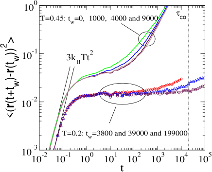
Figure 5: The mean squared displacement (MSD) versus time at temperatures $T\!=\!0.45$ (lines) and $T\!=\!0.2$ (symbols) for various waiting times, $t_{\text{w}}$ (increasing from top to bottom). $t_{\text{w}}\!=\!0$ corresponds to the time of temperature change from $T\!=\!0.5$ to the investigated temperature. While at $T\!=\!0.45$ the time translation invariance (TTI) is reached after a few thousand LJ time units, the data corresponding to $T\!=\!0.2$ indicate an endless evolution towards slower dynamics. The larger $t_{\text{w}}$, the wider the plateau and thus the longer the life time of the cage. The straight lines are fits to the short time behavior of the curves assuming free particle motion with thermal velocity. The vertical dotted line marks $\tau_{\text{c}o}\!=\!2\times 10^{4}$. This time is closely related to a change in the $\dot{\gamma}_{\text{tot}}$-dependence of $\sigma^{\text{peak}}$ [see the discussion of Fig. 8].

III Results at imposed shear rate

An overall shear rate is imposed by moving in the $x$-direction, say, the left wall ($z_{\text{wall}}\!=\!-20$) with a constant velocity of $U_{\text{wall}}$. This defines the total shear rate $\dot{\gamma}_{\text{tot}}\!=\!U_{\text{wall}}/L_{z}$. The motion of the wall is realized in two different ways. One method used in our simulations is to move all wall atoms with strictly the same velocity. In this case, wall atoms do not have any thermal motion. As a consequence, the only way to keep the system temperature constant, is to thermostat the fluid atoms directly. A different kind of wall motion is realized by coupling each wall atom to its equilibrium lattice position via a harmonic spring He-Robbins . In this case, the lattice sites are moved with a strictly constant velocity while each wall atom is allowed to move according to the forces acting upon it [the harmonic forces ensure that the wall atoms follow the motion of the equilibrium lattice sites]. In such a situation, we can thermostat the wall atoms while leaving the fluid particles unperturbed. The temperature of the inner part of the system is then a result of the heat exchange with the walls (which now act as a heat bath). This method has the advantage of leaving the fluid dynamics unperturbed by the thermostat.

The drawback of thermostating the system through the heat exchange with the walls is that, depending on the shear rate and the stiffness of the harmonic spring, measured by the spring constant $k_{\text{h}}$, a temperature profile can develop across the system. Note that the smaller the harmonic spring constant, the better the heat exchange with the walls and thus the more efficient the system is thermostated (the imposed shear rate having the opposite effect). On the other hand, if $k_{\text{h}}$ is too small, the fluid particles may penetrate the walls. We find that $k_{\text{h}}\!=\!25$ is a reasonable choice for our model. However, even with this value of the harmonic spring constant, we observe a temperature profile as the shear rate exceeds $\dot{\gamma}_{\text{tot}}\!=\!10^{-4}$. For $\dot{\gamma}_{\text{tot}}\!=\!10^{-3}$, for example, the maximum temperature in the fluid is by about $3\%$ higher than the prescribed value.

In order to prevent such uncontrolled temperature increases, we have therefore decided to apply direct thermostating to the inner particles at all shear rates, independently of the possibility of the heat exchange with the walls. For this purpose, we divide the system into parallel layers of thickness $dz=0.25$ and rescale (once every 10 integration steps) the $y$-component of the particle velocities within the layer, so as to impose the desired temperature $T$. Such a local treatment is necessary to keep a homogeneous temperature profile when flow profiles are heterogeneous. To check for a possible influence of the thermostat, we compared, for low shear rates ($\dot{\gamma}_{\text{tot}}\leq 10^{-4}$), these results with the output of a simulation where the inner part of the system was unperturbed and the walls were thermostatted instead. Both methods give identical results, indicating that the system properties are not affected by the thermostat.

However, for wall velocities close to $1$ or larger (corresponding to overall shear rates of $\dot{\gamma}_{\text{tot}}\geq 2.5\times 10^{-2}$), a non-uniform temperature profile develops across the system even if the velocities are rescaled extremely frequently footnote2 . This can be rationalized as follows. The heat created by the shear motion needs approximately $t_{c}\!=\!c/L_{z}$ to transverse the system ($c$ is the sound velocity). We can estimate the sound velocity from a knowledge of the shear modulus, $G$, and the density of the system, $c\!=\!\sqrt{G/\rho}$. At $T\!=\!0.2$ we find $G\!\approx\!15$ (see Fig. 6) thus obtaining $c\!\approx\!3.54$. A time of $t_{c}\approx 11.3$ is therefore needed for a signal to transverse the whole system. Note that the heat creation rate is given by $dQ/dt\!=\!\sigma\dot{\gamma}_{\text{tot}}$ (neglecting inhomogeneities in the local shear rate). An amount of energy equal to $k_{\text{B}}T$ is thus generated within $t_{Q}\!=\!k_{\text{B}}T/\dot{Q}$. The requirement $t_{Q}\geq t_{c}$ now means that the heat creation must be slow enough so that the created energy can be dissipated in the whole system efficiently. This gives $\dot{\gamma}_{\text{tot}}\leq k_{\text{B}}T/\sigma t_{c}$, which, after setting $T\!=\!0.2$ and $\sigma\!\approx\!0.6$, yields $\dot{\gamma}_{\text{tot}}\leq 3\times 10^{-2}$.

Figure 6 shows a typical set of (transient) stress-strain curves at a temperature of $T\!=\!0.2$ and for a waiting time of $t_{\text{w}}\!=\!4\times 10^{4}$ LJ time units. The varying parameter is the overall shear rate $\dot{\gamma}_{\text{tot}}\!=\!U_{\text{w}all}/L_{z}$ (the strain is simply computed as $\gamma\!=\!\dot{\gamma}_{\text{tot}}t$). First, an elastic regime is observed at small shear deformations ($\gamma\leq 0.02$). The stress then increases up to a maximum, $\sigma^{\text{peak}}$, before decreasing towards the steady state stress at large deformations. Therefore, this maximum is sometimes referred to as the yield point Utz or dynamical yield stress Khan . In the following, we will simply refer to this quantity as $\sigma^{\text{peak}}$, since plastic (irreversible) deformation actually sets in before the corresponding value of the strain is reached. Moreover, as will be seen below, $\sigma^{\text{peak}}$ depends on strain rate and waiting time in a nontrivial way, so that it is difficult, in our simulations, to define a yield stress value from such dynamical stress/strain curve.

As commonly observed in experiments on polymers Govaert and on metallic glasses vanAken ; Johnson , the stress overshoot $\sigma^{\text{peak}}$ decreases and is observed at smaller strains as the shear rate is lowered [see also Fig. 8]. Note also that all curves in Fig. 6 show the same elastic response at small strains. As also shown in the figure, a linear fit to $\sigma\!=\!G\gamma$ with a shear modulus of $G\!\approx\!15$ describes well the data at small deformations.

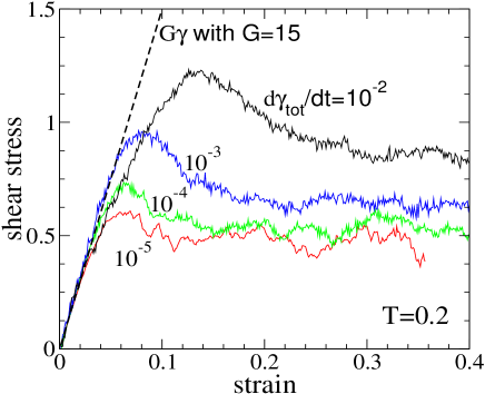
Figure 6: Stress response versus applied strain, $\gamma\!=\!\dot{\gamma}_{\text{tot}}t$, for the strain rates of $\dot{\gamma}_{\text{tot}}\!=\!10^{-5},\;10^{-4},\;10^{-3}$ and $10^{-2}$. Note that both the maximum and the steady state values of the stress decrease with decreasing shear rate. All stress-strain curves coincide with the straight line $\sigma\!=\!G\gamma$ ($G\!\approx\!15$ is the elastic shear modulus) at small deformations ($\gamma\leq 2\%$).

In order to understand the rather strong deviation from linearity at small strains in the case of $\dot{\gamma}_{\text{tot}}\!=\!10^{-2}$, we recall that, once the (left) wall starts its motion, a time of approximately $t_{c}\!=\!11.3$ must elapse before the deformation field comprises the whole system. This is nicely borne out in the inset of Fig. 7 where, for a wall velocity of $U_{\text{w}all}\!=\!0.1$, “snap shots” of the layer resolved displacement of center of mass (normalized to the displacement of the wall) are shown for $t\!=\!1,\;5$ and $11$. Indeed, the boundary of the deformed region reaches the immobile wall only after $t\!=\!11$ LJ time units. We have verified this behavior for other wall velocities and have found $t\!\approx\!11$ in all cases. However, as shown in the main part of Fig. 7, at higher wall velocities, the deformation field is no longer linear at the time it reaches the immobile wall. This can be rationalized as follows. The total strain at $t\!=\!t_{c}$ is given by $\gamma\!=\!\dot{\gamma}_{\text{tot}}t_{c}$ yielding $\gamma\!=\!11\%$ for $\dot{\gamma}_{\text{tot}}\!=\!0.4/40\!=\!10^{-2}$. Hence, the elastic regime is left already before the whole system is affected by the motion of the wall. Putting it the other way, one can estimate the time for which a locally elastic response can still be observed at a given wall velocity: $t_{\text{el.resp.}}\!=\!\gamma_{\text{el}}/\dot{\gamma}_{\text{tot}}$. Assuming an elastic response at a strain of a few percent one obtains for $t_{\text{el.resp.}}$ a time of a few Lennard-Jones units at $\dot{\gamma}_{\text{tot}}\!=\!10^{-2}$ [see the stars in the inset of Fig. 7].

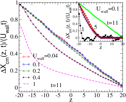
Figure 7: Short time behavior of the layer resolved displacements of the center of mass normalized to the displacement of the moving wall, $(X_{\text{cm}}(z;t)-X_{\text{cm}}(z;0))/(U_{\text{w}all}t)$ ($z$ denotes the position of the middle of the layer. The system is divided into layers of thickness $\Delta z\!=\!1$ and $X_{\text{cm}}$ is measured by averaging over the $x$-coordinates of all particles within the specified layer). The displacement field is shown at $t\!=\!11$ (note that the time needed by the sound to travel across the system is given by $t_{c}\!=\!L_{z}/c\!\approx\!11.3$) for various wall velocities as indicated in the figure. For $U_{\text{w}all}\leq 0.2$, a linear deformation profile is observed, whereas at higher wall velocities this is no longer the case. The inset shows, for a (low) wall velocity of $U_{\text{w}all}\!=\!0.1$, how the deformation field propagates towards the immobile wall (placed at $z\!=\!20$). The speed with which the boundary of the deformed region extends towards the immobile wall is found to be indeed very close to the estimated value of the sound velocity $c\!\approx\!3.54$. The stars in the inset correspond to $U_{\text{w}all}\!=\!0.4$ at $t\!=\!5$ demonstrating that, at a time corresponding to a smaller strain, the local response of the system is elastic [see also the text for more discussion].

The dependence of $\sigma^{\text{peak}}$ on $\dot{\gamma}_{\text{tot}}$ is depicted in Fig. 8 for temperatures of $T\!=\!0.2$ and $T\!=\!0.4$. For the lower temperature, data are shown for two system sizes $L_{x}\!=\!L_{y}\!=\!10,\;L_{z}\!=\!40$ (averaged over 10 independent runs) and $L_{x}\!=\!L_{y}\!=\!L_{z}\!=\!40$ (a sole run). As seen from Fig. 8, for both system sizes, results on $\sigma^{\text{peak}}$ are practically identical. Note that the computation of $\sigma^{\text{peak}}$ at $\dot{\gamma}_{\text{tot}}\!=\!2.5\times 10^{-6}$ for the large system required about 25 days of simulation on a 1.8GHz AMD-Athlon CPU. The data point corresponding to $\dot{\gamma}_{\text{tot}}\!=\!10^{-6}$ has therefore been computed using the average over many small systems only. As the results are not sensitive to the system size, we have used the smaller system size also in the case of $T\!=\!0.4$ (again averaging over $10$ independent runs).

For $T\!=\!0.2$, a change in the slope of $\sigma^{\text{peak}}$-$\dot{\gamma}_{\text{tot}}$-curve is observed at a shear rate of approximately $\dot{\gamma}_{\text{co}}\!=\!2.5\times 10^{-5}$. At shear rates smaller than $\dot{\gamma}_{\text{co}}$, the system seems to have enough time for a partial release of the stress through rearrangements of particles. Note that the stress overshoot $\sigma^{\text{peak}}$ is observed at strains smaller than $5\%$. Therefore, small rearrangements are sufficient in order to release the stress considerably. Indeed, an investigation of the mean squared displacement shown in Fig. 5 reveals that the MSD departs from the plateau for $\tau_{\text{c}o}\!=\!2\times 10^{4}$. This time is of the same order as the inverse of the cross over shear rate thus suggesting that the cross over in the $\dot{\gamma}_{\text{tot}}$-dependence of $\sigma^{\text{peak}}$ is related to the beginning of the cage relaxation. While at higher overall shear rates the response of the system is dominated by the (shorter) time scale imposed by the shear motion, it is no longer the case at $\dot{\gamma}_{\text{tot}}<\dot{\gamma}_{\text{co}}$, where the inherent system dynamics come into play. Although not so pronounced, a similar cross over is seen also in the case of $T\!=\!0.4$ at a larger shear rate in agreement with the observation that, compared to $T\!=\!0.2$, the MSD at $T\!=\!0.4$ leaves the plateau at a shorter time [see the MSD($T\!=\!0.4$) in Fig. 18]. Note that, as the structural relaxation time is approximately proportional to the age of the system barratkob , $\tau_{\text{c}o}$ is of the order of $t_{\text{w}}$. The system response below the crossover is in fact a complex combination of aging dynamics and stress induced relaxation. The aging dynamics tends to make the system stiffer (see below), so that the observed $\sigma^{\text{peak}}$ is higher than the value one would extrapolate from high shear rates.

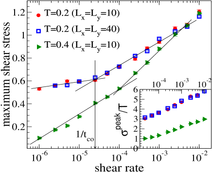
Figure 8: The maximum of the stress-strain curve, $\sigma^{\text{peak}}$, versus strain rate. Data for $T\!=\!0.2$ correspond to two different system sizes: $L_{x}\!=\!L_{y}\!=\!10,\;L_{z}\!=\!40$ (averaged over 10 independent runs) and $L_{x}\!=\!L_{y}\!=\!L_{z}\!=\!40$ (a sole run). Apparently, results on $\sigma^{\text{peak}}$ do not depend much on the system size. At the higher temperature ($T\!=\!0.4$), only the smaller system size (again averaged over 10 independent runs) is used. At approximately $\dot{\gamma}_{\text{tot}}\!=\!2.5\times 10^{-5}$, the slope of $\sigma^{\text{peak}}$ changes significantly at $T\!=\!0.2$. For $T\!=\!0.4$, a similar (albeit not so strong) change in slope occurs at a higher shear rate. Solid lines are guides for the eye. The inset shows the same data, where $\sigma^{\text{peak}}$ divided by temperature is shown versus $\dot{\gamma}_{\text{tot}}$.

The dependence of the stress overshoot $\sigma^{\text{peak}}$ on the imposed shear rate is often expressed with a simple formula which goes back to the Ree-Eyring’s viscosity theory Eyring ; Larson ,

$$\sigma^{\text{peak}}\!=\!\sigma_{0}+k_{\text{B}}T/v^{*}\ln(\dot{\gamma}_{\text{tot}}/\nu_{0}).$$ (1)

Here, the activation volume, $v^{*}$, is interpreted as the characteristic volume of a region involved in an elementary shear motion (hopping) and $\nu_{0}$ is the attempt frequency of hopping. Obviously, Eq. (1) makes sense only at high enough shear rates, for in the case of $\dot{\gamma}_{\text{tot}}<\nu_{0}$, the second term on the right hand side of Eq. (1) becomes negative. Fitting the data of Fig. 8 to Eq. (1), we obtain $v^{*}\!\approx\!2.3$ at $T\!=\!0.2$ and $v^{*}\!\approx\!3.0$ at $T\!=\!0.4$. This result is comparable to the estimates of the free volume from experiments on polycarbonate, where a value of $v^{*}\!\approx\!3.5\text{nm}^{3}$ per segment is reported HoHuu .

Ho Huu and Vu-Khanh HoHuu have extensively studied the effects of physical aging and strain rate on yielding kinetics of polycarbonate(PC) for temperatures ranging from $-80^{\circ}{\text{C}}$ to $60^{\circ}{\text{C}}$ [note that $T_{\text{g}}(\text{PC})\!\approx\!140^{\circ}{\text{C}}$]. In particular, they have measured the tensile stress at yield point, $\sigma^{\text{yt}}$, as a function of strain rate, $\dot{\epsilon}$, for various temperatures and different ages of the sample. As for the effect of temperature, they find that the slope of $\sigma^{\text{yt}}(\ln\dot{\epsilon})/T$ (i.e. the activation volume) is practically independent of $T$. Our data also show only a weak dependence of $v^{*}$ on temperature, as illustrated in the inset of Fig. 8. Note that we have also restricted the data-range to higher shear rates where Eq. (1) is expected to hold better.

The above qualitative agreement on the strain rate dependence of the stress at yield point for our molecular model glass and polycarbonate suggests that, for strains smaller than, say $10\%$, the relevant length scale is that of a segment. In other words, the chain connectivity has a rather subordinate effect on the stress at the yield point (in fact, the connectivity becomes important for larger strains, where the well-known strain hardening sets in Govaert ; Johnson ).

For the same binary mixture of Lennard-Jones particles as in the present work, Rottler and Robbins Rottler studied the dependence of $\tau^{\text{y}}_{\text{dev}}$, the maximum of the deviatoric stress, on the shear rate. In contrast to our results, no crossover similar to that shown in Fig. 8 was observed in this reference. Furthermore, by varying the temperature in the range of $T\in[0.01\;0.3]$ (by a factor of 30), they found that the slope of the $\tau^{\text{y}}_{\text{dev}}$-$\ln\dot{\gamma}_{\text{tot}}$ data did practically not change with temperature, whereas in our case, as discussed above, the slope of $\sigma^{\text{peak}}$-$\ln\dot{\gamma}_{\text{tot}}$ approximately scales with $T$ (see the inset of Fig. 8). Note, however, that in Ref. Rottler a smaller cutoff radius of $r_{\text{c}}\!=\!1.5$ for the Lennard-Jones potential is used, whereas $r_{\text{c}}\!=\!2.45$ in our model. Furthermore, the pressure in Rottler is kept at zero at all temperatures, whereas it is always positive in our simulations. These differences enhance the repulsive (and therefore athermal) character of the system simulated by Rottler and Robbins compared to our model. This also explains why the shear banding is observed at a temperature as low as $T\!=\!0.01$ in Rottler , whereas we observe it at $T\!=\!0.2$ and even higher temperatures VBBB . It is also worth mentioning that the uniaxial strain in Ref. Rottler was imposed by a simple instantaneous rescaling of the box dimension and the positions of all particles, whereas in our case a more realistic situation is considered: The shear strain in the fluid is induced through interactions with a moving atomistic wall. We must however emphasize that, at the present moment, it is not clear how the above differences in details of the model and in the applied simulation techniques may lead to the observed discrepancies in the behavior of the $\sigma^{\text{peak}}$-$\ln\dot{\gamma}_{\text{tot}}$ curve.

As an inspection of Fig. 6 reveals, the difference between the peak and the steady state stresses decreases as $\dot{\gamma}_{\text{tot}}$ is reduced thus suggesting that, in the limit of vanishing shear rate, $\sigma^{\text{peak}}$ converges towards the steady state stress (and therefore coincides with the yield stress that could be extracted from homogeneous flow experiments). Figure 9 compares these two quantities, underlining this expectation further.

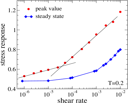
Figure 9: The maximum of the stress-strain curves as shown in Fig. 6, $\sigma^{\text{peak}}$, and the steady state stress versus strain rate for a temperature of $T\!=\!0.2$. For $\sigma^{\text{peak}}$, we average the results for both system sizes shown in Fig. 8.

It has been shown in experiments on amorphous polymers like poly(styrene) and polycarbonate Govaert ; HoHuu that aging strongly alters the response of the system to an applied strain. At small deformations (below, say $5\%$) the slope of the stress-strain curve (elastic shear modulus) increases with progressive aging. Furthermore, the maximum of the stress-strain curve, $\sigma^{\text{peak}}$, is larger for “older” systems and the subsequent decrease of the stress (“strain softening” Govaert ) is more pronounced. Similar observations are also made in experiments on metallic glasses vanAken . Interestingly, Fig. 10 shows that these features are not limited to polymers or metallic glasses but can also occur in simpler models. In Fig. 10 the stress is depicted versus applied strain (defined as $\gamma\!=\!t\dot{\gamma}_{\text{tot}}\!=\!tU_{\text{w}all}/L_{z}$). Before shearing, the system is first equilibrated at a temperature of $T\!=\!0.5$. The motion of the (left) wall is then started at a time $t_{\text{w}}$ after the temperature quench. Varying $t_{\text{w}}$, we observe similar effects on the stress response as described above. It is also observed that, whereas the maximum stress $\sigma^{\text{peak}}$ increases with $t_{\text{w}}$, the elastic shear modulus (slope of the stress-strain curve) seems to saturate already for $t_{\text{w}}\geq 2000$ (this is, however, hardly distinguishable in the scale of the figure).

On the other hand, at large deformations, the stress response does not show any systematic dependence on the age of the system thus indicating a recovery of the time translation invariance: steady shear “stops aging” Kurchan . In fact, it is well known that the shear motion promotes structural relaxation and sets an upper bound ($\sim 1/\dot{\gamma}_{\text{tot}}$) to the corresponding time scale. Once the steady shear state is reached (which is the case at deformations comparable to unity), no dependence on the system age is expected. Results shown in Fig. 10 are also in qualitative agreement with data reported in Ref. Utz , where the system response to a homogeneous shear was studied via Monte Carlo simulations of a binary Lennard-Jones mixture (very close to the present model). Note that, in Ref. Utz , only the contribution to the system response of the so called inherent structure (configurations corresponding to the minima of the energy landscape) has been considered and the effect of aging is investigated by applying different cooling rates (not by “quenching and waiting” as is the case in our work). Despite these differences in details, results reported in Ref. Utz and our observations are quite similar. More quantitative data on the effect of physical aging on the stress at the yield point is shown in the inset of Fig. 10. Here, $\sigma^{\text{peak}}$ is depicted as a function of the waiting time, where $t_{\text{w}}$ is varied by more than four decades. A logarithmic dependence of $\sigma^{\text{peak}}$ on $t_{\text{w}}$ is clearly seen for waiting times larger than a few hundred LJ time units thus covering about three decades in $t_{\text{w}}$. Such an increase in $\sigma^{\text{peak}}$ is consistent with the qualitative idea that the system visits deeper energy minima as aging time increases. A stronger stress is therefore necessary to overcome the energy barriers towards steady flow. It is interesting to note that such a $t_{w}$ dependence of the stress overshoot is also observed in the SGR model Sollich .

As indicated above, simultaneous consideration of figures 8 and 10 indicates a rather complex behaviour of $\sigma^{\text{peak}}$ as a function of $t_{w}$ and $\dot{\gamma}_{\text{tot}}$. Considering the similarity in dependence for large $\dot{\gamma}_{\text{tot}}$ or large $t_{\text{w}}$, it is tempting to suggest a rewriting of equation 1 in the form $\sigma^{\text{peak}}\!=\!\sigma_{0}+k_{\text{B}}T/v^{*}\ln(\dot{\gamma}_{\text{tot}}t_{\text{w}})$. This modified version of Eq. 1 does, however, not describe our data consistently. At $T\!=\!0.2$, for example, the $\sigma^{\text{peak}}/T$ versus $\ln(\dot{\gamma}_{\text{tot}}t_{\text{w}})$ curve exhibits different slopes for the data obtained by varying the imposed shear rate (Fig. 8) as compared to the simulation results where $t_{\text{w}}$ is the adjustable parameter (corresponding to the data shown in the inset of Fig. 10).

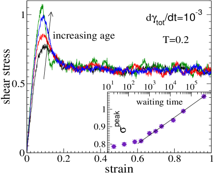
Figure 10: Aging effects on the stress response to an applied strain. $\sigma(\gamma)$ is shown for a strain rate of $\dot{\gamma}_{\text{tot}}\!=\!10^{-3}$ at $t_{\text{w}}\!=\!20,\;2\times 10^{3},\;4.18\times 10^{4}$ and $3.99\times 10^{5}$ LJ time units. At small deformations, the stress increases faster with progressive aging. The maximum observed stress, $\sigma^{\text{peak}}$, is reached at smaller strains and is higher for “older” samples. At large deformations, however, the stress converges towards the same average value regardless of the age of he system. This is a signature of the recovery of time translation invariance, or, equivalently, the erasure of the memory effects due to shear induced structural relaxation. The inset shows the variation of the maximum stress with the waiting time. Note that, here, $t_{\text{w}}$ is varied by more than $4$ orders of magnitude, i.e from $t_{\text{w}}\!=\!20$ to $t_{\text{w}}\!=\!3.99\times 10^{5}$. The solid line is a guide for the eye. The data correspond to a system size of $L_{x}\!=\!L_{y}\!=\!L_{z}\!=\!40$ (a sole run). For the largest waiting time [$t_{\text{w}}\!=\!3.99\times 10^{5}$ ($\!=\!2\times 10^{7}$ MD steps)], however, average over $10$ independent runs of a smaller system size is used ($L_{x}\!=\!L_{y}\!=\!10$, $L_{z}\!=\!40$). Note that already at this (smaller) system size, the size effects are practically negligible [see also Fig. 8].

As for the effect of the temperature on the (transient) stress response, it is generally known that, due to faster structural relaxation at higher $T$, the shear stress decreases at higher temperatures. This is verified in Fig. 11 where stress-strain curves are shown at $T\!=\!0.2,\;0.4,\;0.43$ and $0.5$ for a strain rate of $\dot{\gamma}_{\text{tot}}\!=\!10^{-3}$. Similar to the effect of a decreasing shear rate, both the maximum and the steady state values of the stress decrease with increasing temperature. Furthermore, the slope of stress-strain curves decreases (the system structure “softens”) at higher $T$. Qualitatively similar observations are also made on experimental systems (see, for example, figure 1.20 in Larson , or Refs. Johnson ; Govaert ; vanAken ; HoHuu ). It is also seen from Fig. 11 that a change of temperature by a factor of two in the glassy state (from $T\!=\!0.2$ to $T\!=\!0.4$) has less impact on the maximum stress, $\sigma^{\text{peak}}$, than a smaller $T$-variation close to $T_{\text{c}}$ (from $T\!=\!0.4$ to $T\!=\!0.43$). This illustrates the sensitivity of the yield point to a temperature change in the vicinity of $T_{\text{c}}$. Already from this observation, we can expect a similar impact on the $T$-dependence of the static yield stress (see below) close to the mode coupling critical temperature of the system.

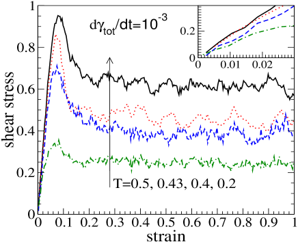
Figure 11: Effect of temperature on the stress response to an applied strain. $\sigma(\gamma)$ is shown for a strain rate of $\dot{\gamma}_{\text{tot}}\!=\!10^{-3}$ at $T\!=\!0.2,\;0.4,\;0.43$ and $0.5$ (note that the mode coupling critical temperature of the system is $T_{\text{c}}\!=\!0.435$). For temperatures below $T_{\text{c}}$ the system was first aged during $t_{\text{w}}\!=\!4\times 10^{4}$ LJ time units before the beginning of the measurement. Similar to the effect of a decreasing shear rate, both the maximum and the steady state values of the stress decrease with increasing temperature. Furthermore, at small strains, the slope of stress-strain curves (elastic shear modulus) decreases increasing temperature (see the inset) thus indicating a softening of the system structure at higher $T$ [compare to Fig. 6]. Note, however, that these changes are much more pronounced in a narrow temperature interval around $T_{\text{c}}$. Results here correspond to averages over $10$ independent runs. The system size was $L_{x}\!=\!L_{y}\!=\!10$ and $L_{z}\!=\!40$. The inset shows a magnification of the small strain region of the same data.

IV Results at imposed stress

In this section we study the response of the system to imposed shear stress. The system is prepared in a similar way as described in previous sections so that, at the beginning of the measurement, the structural relaxation times of the system are much larger than the time scale of the simulation. Starting with $\sigma(t\!=\!0)\!=\!0$, we gradually increase the external stress (i.e. the force acting on the atoms of the left wall) and record quantities of interest, such as the internal energy, the stress across the system, the center of mass velocity of the walls and of the fluid, etc…

It is generally accepted that imposing an external stress leads to a shift in the density of accessible states towards higher energy configurations. For the binary Lennard-Jones model of the present work, Fig. 12 shows the potential energy per particle, $e_{\text{pot}}$, as measured in simulations where the imposed stress is periodically varied the range $\sigma\in[-0.8\;0.8]$ (see the zigzag line in Fig. 12. Similar stress ramps were also used by He and Robbins He-Robbins in order to determine the static friction between two solid bodies mediated by a layer of adsorbed molecules).

Note that the maxima and minima of the potential energy correspond to $|\sigma|\!=\!0.8$ and $\sigma\!=\!0$ respectively. Starting at a minimum of $e_{\text{pot}}$ ($\sigma\!=\!0$), the potential energy fluctuates for a while around this minimum before increasing sharply towards a maximal value. This corresponds to a branch where $|\sigma|$ increases from $0$ to $0.8$. The descent from this maximum towards the subsequent minimum ($|\sigma|$ decreases from $0.8$ to $0$) is, however, more gradual and indicates a dependence of $e_{\text{pot}}$ on the stress history. Finally, we also observe that, at high $\dot{\sigma}$, the quiescent energy distribution observed at small stresses at the very beginning of the stress ramp simulation, is never reached again whereas the stress itself passes through zero periodically. This dependence on $\dot{\sigma}$, however, is considerably weakened as the stress increase rate reaches values below $5\times 10^{-5}$.

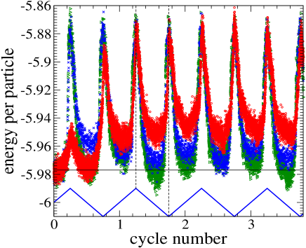
Figure 12: Effect of the rate of stress increase on potential energy per particle. $e_{\text{pot}}$ is measured during cyclic variations of the imposed stress as sketched by the zigzag line (note that $\sigma$ varies in the range $[-0.8\;0.8]$). The horizontal axis counts the number of cycles. Three rates of stress variation are shown here, $\dot{\sigma}\!=\!5\times 10^{-4},\;5\times 10^{-5}$ and $10^{-5}$. T he higher $\dot{\sigma}$, the higher the potential energy per particle at small stresses (minimum of $e_{\text{pot}}$). The vertical dashed lines mark simultaneously the maxima of $e_{\text{pot}}$ and $|\sigma|$. They serve to better recognize the asymmetry of $e_{\text{pot}}$ on both sides of the stress maximum and recall the presence of a hysteresis effect.

While the potential energy per particle is easily measured in a simulation, this is not the case in real experiments. The velocity of the solid boundary (upon which the stress acts), however, is experimentally accessible. Figure 13 depicts the wall velocity measured in simulations at $\dot{\sigma}\!=\!5\times 10^{-5}$. Following the convention, the applied stress is shown on the vertical axis, whereas on the horizontal axis the system response is depicted. We first note that, at small stresses, the system resists to the imposed stress and thus prevents the wall from moving. Only when the magnitude of the stress exceeds a certain (yield) value, a non-vanishing wall velocity is observed. Furthermore, after a cross over regime around the threshold value of the stress, the wall velocity increases almost linearly with stress increment.

On the other hand, as the magnitude of the stress is decreased again, the wall motion first slows down along the same line as in the stress increase case but then departs towards higher wall velocities. A hysteresis loop is thus formed as expected from an analysis of the asymmetry of $e_{\text{pot}}$ around the stress maximum [see Fig. 12]. Similar observations are made in experiments on pastes, glass beads, dense colloidal suspensions DaCruz and foams Debregeas::PRL87 . Note also that, as expected from the symmetry of the system response with respect to positive and negative stresses, the shape of the observed hysteresis loop is identical for both directions (signs) of the applied stress.

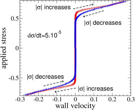
Figure 13: The applied shear stress (vertical axis) and the resulting wall velocity (horizontal axis) measured during stress ramps with a rate of $\dot{\sigma}\!=\!5\times 10^{-5}$. The result shown here is an average over two independent runs each containing 15 full cycles of stress variation [see the zigzag line in Fig. 12].

Next, we investigate the dependence of the system response to an applied stress on the rate of stress variation. For this purpose, $\dot{\sigma}$ is varied by two orders of magnitude, from $5\times 10^{-4}$ to $5\times 10^{-6}$. Figure 14 depicts stress ramp data now averaged using the symmetry with respect to negative and positive stresses. Again, for all values of $\dot{\sigma}$ shown in this figure, no flow is observed for too small stresses (below, say $0.4$). However, for a given stress above, say, $\sigma\!=\!0.7$, the wall velocity is lower at higher $\dot{\sigma}$. To put it the other way, when $|\sigma|$ is increased faster, a given wall velocity is reached at a higher $|\sigma|$, i.e. on a later time. This may be rationalized by noting that, at a higher stress increase rate, the system has less time to develop a response corresponding to the actual (instantaneous) stress. Therefore, the mobility increase corresponding to an increase of the stress is retarded and is observed later, i.e. at higher stress.

However, it is also seen from Fig. 14 that, already at $\dot{\sigma}\leq 2\times 10^{-5}$, the effect of $\dot{\sigma}$ on the system response is of order of the measurement uncertainty, so that no systematic dependence on $\dot{\sigma}$ can be seen for $\dot{\sigma}\leq 2\times 10^{-5}$. This is consistent with the behavior of the potential energy per particle which becomes practically independent of $\dot{\sigma}$ in the same $\dot{\sigma}$-range [see Fig. 12]. Therefore, we may describe this regime of slow variation of $\sigma$ as quasistatic.

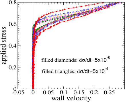
Figure 14: The hysteresis loops as measured during stress ramps with rates of stress variation of $\dot{\sigma}\!=\!5\times 10^{-6}$ (filled diamonds), $2\times 10^{-5},\;5\times 10^{-5},\;10^{-4},\;2\times 10^{-4}$ and $5\times 10^{-4}$ (filled triangles). The $\dot{\sigma}\!=\!5\times 10^{-6}$-curve is an average over $10$ independent runs with a unique variation of the stress from $0$ to $0.76$. The remaining curves correspond to averages over two independent runs each containing many full cycles of stress variation in the intervall $[-0.8\;\;0.8]$. The innermost loop (filled diamonds) corresponds to the smallest $\dot{\sigma}$. Note that the surface of the hysteresis loop increases at higher stress variation rates thus indicating stronger retardation effects. Note also that, for the two highest $\dot{\sigma}$, the loop does not close within the simulated stress range. It would close at much higher stresses than shown in the figure.

Results presented above and in previous works BB::PRE61::2000 ; BB2 show that our model system shares many features of the so called soft glassy materials. In particular, the existence of a yield stress is suggested in Figs. 13 and 14. Figure 15 displays further evidence of the existence of a yield stress still as the dramatic change in the wall velocity at a threshold stress value is emphasized using a logarithmic scale for the horizontal axis. In a narrow stress range around $\sigma\!=\!0.6$, the wall velocity and thus the overall shear rate increases approximately by three orders of magnitude [see also Fig. 1]. Again, a linear regime is observed at high stresses DaCruz . Besides the hysteresis already discussed above, an investigation of the decreasing branch on the stress-wall velocity curve in Fig. 15 reveals that, as $\sigma$ falls below a certain value, the wall velocity becomes even negative [see the inset]. This clearly illustrates the presence of attractive forces which, now, are stronger than the imposed stress and thus capable of reducing the amount of strain. Indeed, an inspection of the center of mass position of the wall and of the fluid shows that both these quantities exhibit a maximum at the place where the velocity passed through zero (as the stress is further reduced, $X_{\text{cm}}$ decreases in accordance with the observation of a negative velocity). Very similar observations are also reported on the experimental side DaCruz .

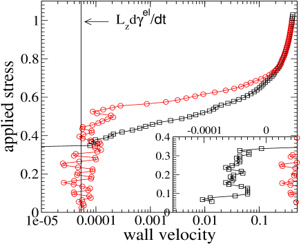
Figure 15: The applied shear stress (vertical axis) and the resulting wall velocity (horizontal axis) measured during stress ramps with a rate of $\dot{\sigma}\!=\!2\times 10^{-5}$. The vertical solid line roughly marks the elastic contribution to the strain rate ($\dot{\gamma}^{\text{el}}\!\approx\!\dot{\sigma}/G$. Elastic deformation gives rise to a non vanishing wall velocity even at the smallest imposed stress. See also Fig. 6 for an estimation of the shear modulus $G$). The inset shows that, as the stress is decreased, the wall velocity changes its sign thus indicating that the attractive forces are stronger than the imposed stress so that the direction of deformation is reversed in order to reduce the amount of the accumulated strain.

V Measurement of the yield stress

As discussed in section I, there seems to be a close connection between the existence of a yield stress and the observation of the shear banding phenomenon in many soft glassy materials CoussotJRheh46 ; DaCruz ; VBBB . In particular, it is commonly expected that, in a state where the yield stress vanishes (at high temperatures, for example) the shear bands should also disappear, i.e. the whole system should flow. In addition to this experimental aspect, a study of the yield stress is also motivated from the theoretical point of view. For example, the so called soft glassy rheology model (SGR) of Sollich Sollich2 (an extension of the trap model Bouchaud taking into account yielding effects due to an external flow) predicts a linear onset of the dynamic yield stress as the glass transition is approached, $\sigma(\dot{\gamma}_{\text{tot}}\to 0)\sim 1-x$. Here, $x$ is a noise temperature, $x\!=\!1$ corresponds to the glass transition (or “jamming”) temperature, and $x<1$ characterizes the glassy or “jammed” phase. On the other hand, numerical studies of a $p$-spin mean field Hamiltonian BB::PRE61::2000 predict that the dynamic yield stress vanishes at all temperatures. There has recently been a more microscopic approach based on an extension to non equilibrium situation FuchsCates of the mode coupling theory of the glass transition (MCT) MCTRefs . An analysis of schematic models within this approach shows a rather discontinuous change in the dynamic yield stress at the mode coupling critical temperature, $T_{\text{c}}$.

The reader may have noticed that the above mentioned theories make predictions on the dynamic yield stress [defined as $\sigma(\dot{\gamma}_{\text{tot}}\to 0)$]. Our interpretation of the shear banding, however, makes use of the idea of resistance to an applied stress which is related to the presence of a static yield stress. Similar to the difference between the dynamic and static friction RobbinsMueser , the static and the dynamic yield stresses are not necessarily identical. Indeed, for our model glass, we find that $\sigma_{\text{y}}>\sigma(\dot{\gamma}_{\text{tot}}\to 0)$ [see Fig. 2]. Therefore, a measurement of the static yield stress gives at least an upper bound for the dynamic counterpart. As we will see below, the static yield stress decreases rather sharply as the mode coupling critical temperature of the model ($T_{\text{c}}\!=\!0.435$) is approached. Unfortunately, when measuring $\sigma_{\text{y}}$ at temperatures close to $T_{\text{c}}$, one is faced with the problem that the time scale imposed by the external force (which if of order of the inverse stress variation rate, i.e. $t_{\dot{\sigma}}\!=\!\sigma/\dot{\sigma}$) and that of the (inherent) structural relaxation, $\tau_{\text{relax}}$, are not well separated. In particular, the condition $t_{\dot{\sigma}}\ll\tau_{\text{relax}}$ is not valid at temperatures close to $T_{\text{c}}$. Therefore, as will be discussed below in more details, a conclusive statement on the interesting limit of $\sigma_{\text{y}}(T\to T_{\text{c}})$ can still not be made.

Preliminary results on the static yield stress have been recently obtained within the driven mean field $p$-spin models Berthier . Using the fact that the free energy barriers are finite at finite system size, the model has been investigated by Monte Carlo simulations in the case of $p\!=\!3$ for a finite number of spins, thus allowing the thermal activations to play a role which they could not play in the case of an infinite system size. Results of these simulations support the existence of a critical driving force below which the system is trapped (’solid’) and above which it is not (’liquid’) Berthier . Results based on this new approach on the temperature dependence of the yield stress and, in particular, on its behavior close to $T_{\text{c}}$ are, however, lacking at the moment.

Here, we adopt a method very close to a determination of the (static) yield stress in experiments, i.e. we use the definition of $\sigma_{\text{y}}$ as the smallest stress at which a flow in the system is observed. As we are interested in a study of the temperature dependence of $\sigma_{\text{y}}$ and, in particular, in $\sigma_{\text{y}}(T)$ close to the mode coupling critical temperature, we have varied the temperature in the range of $T\in[0.1\;0.44]$ (recall that $T_{\text{c}}\!=\!0.435$). For each temperature, $\sigma$ was increased stepwise by an amount of $d\sigma\!=\!0.02$ once in each $1000$ LJ time units during which the velocity profile corresponding to the imposed stress is measured. Among other quantities, we also monitor the motion of the center of mass of the wall and also of the fluid itself. Note that the overall stress increase rate in these simulations is $\dot{\sigma}\!=\!2\times 10^{-5}$, and thus corresponds to a quasi static variation of the stress [see the discussion of Figs. 12 and 14]. For each temperature, the simulation was performed using 10 independent initial configurations.

Recall that there is always an elastic contribution to the system response to an applied stress. The corresponding center of mass velocity can simply be estimated as $V^{\text{el}}_{\text{cm}}\!=\!\dot{\sigma}/G$. This contribution is negligible at lower $T$ for two reasons: (i) due to the high stiffness of the system (large $G$), $V^{\text{el}}_{\text{cm}}$ is relatively small and (ii) the onset of the shear motion is quite sharp at low $T$ thus leading to much higher velocities (compared to $V^{\text{el}}_{\text{cm}}$) as soon as the applied stress exceeds $\sigma_{\text{y}}$. In contrast, close to $T_{\text{c}}$, the shear modulus is quite small [see, for example, the slope of the stress-strain curve at $T\!=\!0.43$ in Fig. 11] thus leading to a larger $V^{\text{el}}_{\text{cm}}$. Furthermore, there is no sharp variation in $V_{\text{cm}}$ as a function of applied stress. For a measurement of $\sigma_{\text{y}}$ close to $T_{\text{c}}$, it is therefore important to correct for the elastic contribution to the system response. For this purpose, we have determined the $T$-dependence of the shear modulus. The center of mass velocity of the fluid has then been corrected subtracting, for each temperature, the corresponding $V^{\text{el}}_{\text{cm}}\!=\!\dot{\sigma}/G$.

Figure 16 depicts the applied stress (vertical axis) and the resulting (corrected) center of mass velocity of the fluid, $V_{\text{cm}}$, averaged over all independent runs (horizontal axis). A log-log plot is used in order to emphasize the continuous variation of $V_{\text{cm}}$ with decreasing stress at high temperatures. Contrary to low temperatures ($T\leq 0.35$) where a plateau followed by a sharp drop towards zero in $V_{\text{cm}}$ is observed, the center of mass velocity of the fluid at high temperatures decreases rather continuously for small stresses.

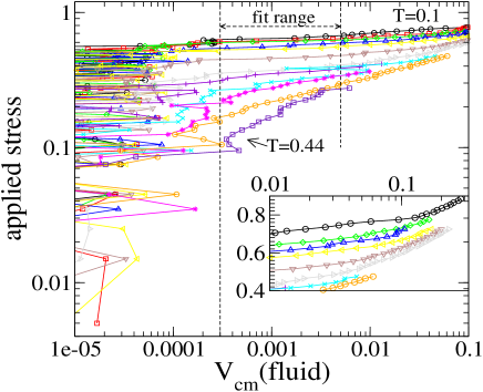
Figure 16: Effect of the temperature on the response of the system to imposed shear stress. The imposed stress is shown on the vertical axis while the center of mass velocity of the fluid (inner part of the system) is depicted as horizontal axis. Each curve corresponds to an average over 10 independent runs. The stress was increased stepwise by an amount of $d\sigma\!=\!0.02$ once in each $dt\!=\!1000$ LJ time units ($\dot{\sigma}\!=\!2\times 10^{-5}$). Note that the contribution of the elastic deformation to the center of mass velocity ($V^{\text{el}}_{\text{cm}}\!\approx\!L_{z}\dot{\sigma}/(2G)$, using the value of $G\!\approx\!15$ at $T\!=\!0.2$) has already been subtracted from the data. Note also that the statistical uncertainty of $V_{\text{cm}}$ is approximately of order of $10^{-4}$. The vertical dashed lines show the limits of the $V_{\text{cm}}$-range used in the fit to $\sigma\!=\!\sigma_{\text{y}}+aV_{\text{cm}}$. The inset is a magnification of the high stress regime.

As a first attempt to determine the yield stress, we apply linear fits to the data shown in Fig. 16. As shown in the same figure, the chosen fit range roughly corresponds to the plateau region at low temperatures. For $T\leq 0.35$, we thus expect the fit result not to be significantly different from the “real” value of $\sigma_{\text{y}}$. However, as an investigation of the high-$T$ behavior of $V_{\text{cm}}$ in Fig. 16 suggests, this method is not expected to give accurate results for $\sigma_{\text{y}}$ at high temperatures ($T\geq 0.38$, say).

A slightly different approach in determining $\sigma_{\text{y}}$ is to find the smallest stress for which the center of mass velocity exceeds a certain, small value, $V^{\text{min}}_{\text{cm}}$. Here, we further require that $V_{\text{cm}}$ must remain larger than $V^{\text{min}}_{\text{cm}}$ for all subsequent stresses. This last condition serves to reduce errors due to fluctuations of $V_{\text{cm}}$. In applying this definition, we use the result of each independent run on $V_{\text{cm}}$ separately and thus obtain, for each $V^{\text{min}}_{\text{cm}}$, a set of yield stress values. This allows an estimate of the statistical error. Figure 17 compares the yield stress obtained via the linear fit to $V_{\text{cm}}$ with results of the second approach for $V^{\text{min}}_{\text{cm}}\!=\!10^{-4},\;10^{-3}$ and $10^{-2}$. Not unexpectedly, it is seen from Fig. 17 that the quality of results on $\sigma_{\text{y}}$ strongly depends on temperature. At temperature far enough from $T_{\text{c}}$, say, for $T<0.35$, $\sigma_{\text{y}}$ is rather insensitive to a change of $V^{\text{min}}_{\text{cm}}$ (differences caused by various choices of $V^{\text{min}}_{\text{cm}}$ are of order of the statistical error). At higher temperatures, however, the variation of $\sigma_{\text{y}}$ with the choice of $V^{\text{min}}_{\text{cm}}$ is remarquable: At $T\!=\!0.43$ it varies between $0.14$, $0.22$ and $0.33$ for $V^{\text{min}}_{\text{cm}}\!=\!10^{-4},\;10^{-3}$ and $10^{-2}$. Therefore, result on $\sigma_{\text{y}}$ at temperatures close to $T_{\text{c}}$ should be considered as rough estimates only.

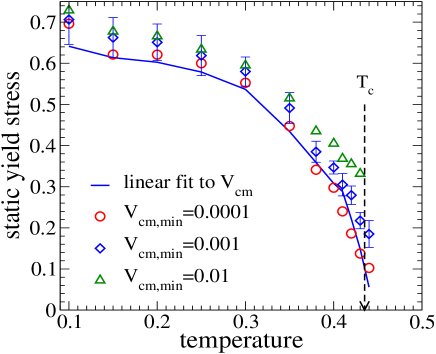
Figure 17: The effect of the temperature on the static yield stress, $\sigma_{\text{y}}$. The solid line shows $\sigma_{\text{y}}$ obtained from fits to $\sigma\!=\!\sigma_{\text{y}}+aV_{\text{cm}}$ ($a$ and $\sigma_{\text{y}}$ are fit parameters) using the fit range $V_{\text{cm}}\in[0.0003\;0.005]$ [see Fig. 16]. The symbols correspond to $\sigma_{\text{y}}$ defined as the smallest stress for which (and for all subsequent higher stresses) the wall velocity exceeds a certain minimum value, $V^{\text{min}}_{\text{cm}}$. Three choices of $V^{\text{min}}_{\text{cm}}$ are compared: $10^{-4}$ (circles), $10^{-3}$ (diamonds) and $10^{-2}$ (triangles). While $\sigma_{\text{y}}$ is relatively insensitive to a choice of $V^{\text{min}}_{\text{cm}}$ at low temperatures, it is not the case for temperatures close to $T_{\text{c}}$, where it continuously decreases as the $V^{\text{min}}_{\text{cm}}$ is reduced. The vertical arrow marks the mode coupling critical temperature $T_{\text{c}}\!=\!0.435$. For clarity, error bars are shown for the case of $V^{\text{min}}_{\text{cm}}\!=\!10^{-3}$ only.

The origin of the difficulty in estimating the static yield stress of the system at temperatures close to $T_{\text{c}}$, can be understood by comparing the time scales relevant to the problem. First, there is a time scale related to the imposed stress $t_{\dot{\sigma}}\!=\!\sigma/\dot{\sigma}$. The second relevant time scale is that of the structural relaxation, $\tau_{\text{relax}}$. The static yield stress is well defined in the limit of a quasi static variation of stress, i.e. $\dot{\sigma}\to 0$ ($t_{\dot{\sigma}}\to\infty$) while at the same time keeping $\tau_{\text{relax}}\gg t_{\dot{\sigma}}$. Using $\sigma\!\approx\!0.5$ and $\dot{\sigma}\!=\!2\times 10^{-5}$ (note that this value of $\dot{\sigma}$ was used at all temperatures in order to determine the yield stress) we obtain $t_{\dot{\sigma}}\!\approx\!2\times 10^{4}$. We are therefore led to verify if the condition $\tau_{\text{relax}}\gg 2\times 10^{4}$ is satisfied at all temperatures. For this purpose, we define $\tau_{\text{relax}}$ as the time needed by the mean square displacement of a tagged particle to reach the particle size. Figure 18 shows the mean square displacement of the unsheared system for $T\in[0.1\;0.44]$ (recall that $T_{\text{c}}\!=\!0.435$). For all these temperatures, the waiting time between the temperature quench (from an initial temperature of $T\!=\!0.5$ to the actual temperature) and the beginning of the measurement was $t_{\text{w}}\!=\!1.8\times 10^{4}$. At low temperatures, the MSD practically remains on a plateau for the whole duration of the simulation indicating that $\tau_{\text{relax}}$ is much larger than the simulated time of $2\times 10^{4}$ LJ time units. At higher temperatures ($T\geq 0.41$), however, after a long plateau, the MSD eventually enters the diffusive regime and reaches a value comparable to unity within the simulated time window. Obviously the condition $\tau_{\text{relax}}\gg t_{\dot{\sigma}}$ is violated at these temperatures. Hence at least for a waiting time of $t_{\text{w}}\!=\!4\times 10^{4}$ and for the choice of $\dot{\sigma}\!=\!2\times 10^{-5}$, the computed static yield stress is not well defined close to $T_{\text{c}}$.

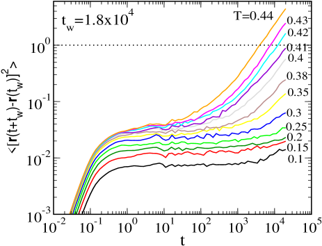
Figure 18: The mean square displacement (MSD) of a tagged particle averaged over all three spatial directions at various temperatures ranging from the supercooled state ($T\!=\!0.44>T_{\text{c}}\!=\!0.435$) down to the frozen state $T\!=\!0.1$. The time $t_{\text{w}}$ indicates the time elapsed between the temperature quench and the beginning of the measurement. At a time of $t\!=\!2\times 10^{4}$, the MSD hardly leaves the plateau at low temperatures. For temperatures $T\geq 0.41$, however, it approximately reaches the size of a particle within the same time interval indicating that a complete structural relaxation has taken place. The horizontal dotted line marks $\text{MSD}\!=\!1$.

VI Conclusion

Results on the yield behavior of a model glass (a 80:20 binary Lennard-Jones mixtures Kob-Andersen ), studied by means of molecular dynamics simulations, have been reported. One of the major motivations of the present work is the observation of shear localization (below the glass transition temperature and at low shear rates) in the present model and the suggestion of a link between this phenomenon and the existence of a static yield stress VBBB (under applied stress, the system does not flow until the stress exceeds a threshold value). A particular emphasis thus lies on the yield stress and its dependence on temperature.

First, the system stress-strain curve under startup of steady shear has been studied. The effect of physical aging (characterized by the waiting time, $t_{\text{w}}$), shear rate ($\dot{\gamma}_{\text{tot}}$), and temperature on the stress-strain relation has been investigated. Regardless of these parameteres, all observed stress-strain curves first exhibit an elastic regime at small shear deformations ($\gamma\leq 0.02$). The stress then increases up to a maximum, $\sigma^{\text{peak}}$, before decreasing towards the steady state stress at large deformations. The steady state stress (corresponding to large deformations) shows a dependence on temperature and on the applied shear rate, but is independent of the system history, indicating a recovery of the time translation invariance due to shear induced structural relaxation BB::PRE61::2000 . In contrast, the stress overshoot $\sigma^{\text{peak}}$, (the first maximum of the stress-strain curves, spmetimes described as a dynamical yield stress) depends on the imposed shear rate and on the waiting time (physical aging). It is observed that, at relatively high shear rates or for large waiting times, the maximum stress increases with $\ln(\dot{\gamma}_{\text{tot}})$ or with $\ln(t_{\text{w}})$, respectively. These observations are consistent with experiments on amorphous polymers Govaert ; vanAken and on metallic glasses HoHuu ; Johnson , and also correspond to the behaviour predicted using the soft glassy rheology model Sollich .

For shear rates below a certain, cross over shear rate, $\dot{\gamma}_{\text{co}}$, however, a decrease in the slope of $\sigma^{\text{peak}}$-$\dot{\gamma}_{\text{tot}}$ curve is seen. A comparison with the steady state shear stress suggests that $\sigma^{\text{peak}}$ saturates at the steady state stress level as the imposed shear rate approaches zero. Moreover, an analysis of the mean square displacements of the unsheared system reveals that the cross over shear rate, $\dot{\gamma}_{\text{co}}$, is very close to $1/\tau_{\text{c}o}$, where $\tau_{\text{c}o}$ marks the time for which the mean square displacement gradually departs from the plateau-regime [see Fig. 5]. We therefore associate this crossover with the beginning of the cage relaxation, which leads to the possibility of small (compared to the size of a particle) rearrangements thus allowing at least a partial release of the stress. $gammadotco$ is also comparable to the inverse of the waiting time: for $gammadottot<gammadotco$, the response of the system is directly influenced by the aging dynamics.

In order to build a closer connection between our studies and typical rheological experiments, stress ramp simulations are performed and the system response is analyzed for stress increase rates ranging from $\dot{\sigma}\!=\!5\times 10^{-4}$ to $\dot{\sigma}\!=\!5\times 10^{-6}$. In agreement with experiments on complex systems like pastes, dense colloidal suspensions DaCruz and foams Debregeas::PRL87 , hysteresis loops in the system response are observed. These loops become wider as $\dot{\sigma}$ increases. An analysis of the potential energy per particle for different $\dot{\sigma}$ nicely shows how high energy configurations are favored by the faster stress variations. This also yields an estimate of quasi static stress application. We find that, for our model, $\dot{\sigma}\!=\!2\times 10^{-5}$ is slow enough so that simulations with this stress variation rate can be used in order to obtain a reliable estimate of the static yield stress.

Finally, the static yield stress, $\sigma_{\text{y}}$, is determined and its reliability is discussed. Our numerical results confirm the observation of reference VBBB , that the static yield stress is higher than the low shear rate limit $\sigma(\dot{\gamma}\rightarrow 0)$ observed in steady shear experiments. The system can therefore produce shear bands for stresses in the range [$\sigma(\dot{\gamma}\rightarrow 0)$,$\sigma_{\text{y}}$].

At temperatures far below the mode coupling critical temperature of the model ($T_{\text{c}}\!=\!0.435$), a slight increase of $\sigma_{\text{y}}$ with further cooling is observed. At temperatures close to $T_{\text{c}}$, however, the static yield stress strongly decreases as $T$ is increased towards $T_{\text{c}}$. As to the reliability of the data, relatively accurate estimate of $\sigma_{\text{y}}$ is obtained at low temperatures (for $T\leq 0.35$). Results on the yield stress at temperatures close to $T_{\text{c}}$, however, are very sensitive to the applied criterion. An investigation of the dynamics of the unperturbed system reveals that, for $T$ close to $T_{\text{c}}$, the structural relaxation times are far from being large compared to the time scale imposed by the external force (the inverse of the stress increase rate, $\sigma/\dot{\sigma}$). Therefore, for the simulated waiting time of $4\times 10^{4}$, the static yield stress is no longer well defined at these high temperatures. This underlines the fact that a very good separation of time scales between the experimental and intrinsic time scales is necessary in order to properly define a static yield stress.

It must, however, be emphasized that, even though an increase of $\dot{\sigma}$ apparently leads to a validity of $\tau_{\text{relax}}\gg t_{\dot{\sigma}}$, this would violate the condition of a quasi static variation of the stress. A more physical way to improve the accuracy of results on $\sigma_{\text{y}}$ is to increase the waiting time, in order to allow $\tau_{\text{relax}}$ to grow beyond $t_{\dot{\sigma}}$. Noting that, at higher temperatures (but still below $T_{\text{c}}$), $\tau_{\text{relax}}$ increases less strongly with $t_{\text{w}}$ (interrupted aging), the limit of large $\tau_{\text{relax}}$ becomes progressively more time consuming in terms of computation time.

Our numerical study shows that a very simple model, studied numerically on relatively short time scales, can exhibit most of the complex rheological behaviour of soft glassy systems, but also of ”hard” (metallic) glasses (it is interesting in this respect to note that the simulated system was originally intended to mimic a NiPd metallic glass). This suggests that these features are generic to most glassy systems, although in practice the values of the parameters may considerably vary from system to system.

References

- (1) W. Kob and H.C. Andersen, Phys. Rev. E 52, 4134 (1995); W. Kob, J. Phys.: Condens. Matter 11, R85 (1999), and references therein. Our unit of time is , differing by a factor from the one used in this reference. Note also that confinement effects can modify the time scale for structural relaxation, and therefore the glass transition temperature as discussed by P. Scheidler et al., Europhys. Lett., in press (2002) for the present model and by F. Varnik et al., Phys. Rev. E 65, 021507 (2002) for a confined polymer melt. The temperatures we consider are low enough that this effect can be ignored for layers not too close to the walls (typically at distances from the wall).
- (2) F. Varnik, L. Bocquet, J.-L. Barrat, L. Berthier Phys. Rev. Lett. 90, 095702 (2003).
- (3) E.M. Arruda, M.C. Boyce and R. Jayachandran, Mechanics of Materials 19, 193 (1995); L.E. Govaert, H.G.H. van Melick and H.E.H. Meijer, polymer 42, 1271 (2001); H.G.H. van Melick, L.E. Govaert and H.E.H. Meijer, polymer 44, 3579 (2003).
- (4) B. van Aken, P. de Hey and J. Sietsma, Materials Science & Engineering A 278, 247 (2000).
- (5) C. Ho Huu and T. Vu-Khanh, Theoretical and Applied Fracture Mechanics 40, 75 (2003).
- (6) W.L. Johnson, J. Lu and M.D. Demetriou, Intermetallics 10, 1039 (2002).
- (7) F. Da Cruz, F. Chevoir, D. Bonn, P. Coussot Phys. Rev. E 66 051305 (2002).
- (8) G. Debrégeas, H. Tabuteau, and J.-M. di Meglio, Phys. Rev. Lett. 87, 178305 (2001).
- (9) P. Sollich, F. Lequeux, P. Hébraud, M.E. Cates, Phys. Rev. Lett. 78, 2020 (1997); S. M. Fielding, P. Sollich, M. E. Cates, J. Rheol., 44, 323 (2000).
- (10) D. Bonn, P. Coussot, H.T. Huynh and F. Bertrand, Europhys. Lett. 59, 786 (2002).
- (11) P. Coussot et al, Phys. Rev. Lett. 88, 218301 (2002).
- (12) R.G. Larson, The structure and Rheology of Complex Fluids (Oxford University Press, New York) 1999.
- (13) D. Bonn, S. Tanase, B. Abou, H. Tanaka and J. Meunier, Phys. Rev. Lett. 89, 015701 (2002).
- (14) F. Pignon, A. Magnin, and J.-M. Piau, J. Rheol., 40, 573 (1996).
- (15) W. Kob and J.-L. Barrat, Phys. Rev. Lett. 78, 4581 (1997); Europhys. Lett. 46, 637 (1999); Eur. Phys. J. B 13, 319 (2000).
- (16) L. Berthier, J.-L. Barrat and J. Kurchan, Phys. Rev. E 61, 5464 (2000); J.-L. Barrat and L. Berthier, Phys. Rev. E 63, 012503 (2000).
- (17) J. Kurchan cond-mat/9812347 (1998), cond-mat/0011110 (2000);
- (18) L. Berthier and J.-L. Barrat, J. Chem. Phys. 116, 6228 (2002); Phys. Rev. Lett. 89, 095702 (2002).
- (19) See, however, D.J. Lacks, Phys. Rev. Lett. 87, 225502 (2001), for an investigation of shear thinning in terms of potential energy landscape.
- (20) See e.g. C.-Y.David Lu, P.D. Olmsted, R.C. Ball, Phys. Rev. Lett. 84, 642 (2000) which also contains many references to relevant experimental work.
- (21) J.K.G. Dhont, Phys. Rev. E 60, 4534 (1999); X.F. Yuan, Europhys. Lett. 46, 542 (1999).
- (22) L.J. Chen, B.J. Ackerson, C.F. Zulowski, J. Rheol, 38, 193 (1993).
- (23) W. Losert, L. Bocquet, T.C. Lubensky and J.P. Gollub, Phys. Rev. Lett. 85, 1428 (2000).
- (24) If there is no such region, the yield stress is necessarily smaller than the steady state stress at the imposed shear rate. This, however, is impossible, for the startup of the shear motion in response to an imposed stress leads to at least a partial release of the stress.
- (25) P. Coussot, Q.D. Nguyen H.T. Huynh and D. Bonn, J. Rheol. 46, 573 (2002).
- (26) A. Lemaitre, preprint cond-mat/0206417.
- (27) C. Dérec, A. Ajdari, G. Ducouret and F. Lequeux, C.R. Acad. Sci. Paris IV 1 1115 (2000); C. Dérec, A. Ajdari and F. Lequeux Eur. Phys. J. E 4 355 (2001).
- (28) G. Picard, A. Ajdari, L. Bocquet, F. Lequeux, Phys. Rev. E 66, 051501 ( 2002).
- (29) G. He and M.O. Robbins Phys. Rev. B. 64 035413 (2001).
- (30) Note that, by choosing a smaller integration time step and applying the rescaling procedure more frequently, one can increase the effective thermostating rate. However, a thermostating rate larger than , ( is the decay time of the velocity auto correlation function) does not make much sense as the heat transferred to the -component of the particle velocities must be first dissipated to the other directions before it can be removed by a rescaling of, say -component of the particle velocities.
- (31) M. Utz, P.G. Debenedetti and F.H. Stillinger, Phys. Rev. Lett. 84 1471.
- (32) H.J. Walls, S.B. Caines, A.M. Sanchez and S.A. Khan, Journal of Rheology, 47, 847 (203) and references therein.
- (33) Jörg Rottler and Mark O. Robbins, cond-mat/0303276.
- (34) H. Eyring, J. Chem. Phys. 4, 283 (1936); T. Ree and H. Eyring in: F.R. Eirich(Ed.), Rheology, vol. II, (Academic Press, New York, 1958), pp. 83-144 (Chapter III).
- (35) P. Sollich, Phys. Rev. E 58, 738 (1998).
- (36) J.P. Bouchaud, J. Phys. I 2, 1705 (1992); C. Monthus and J.P. Bouchaud, J. Phys. A 29, 3847 (1996).
- (37) M. Fuchs and M.E. Cates, Phys. Rev. Lett. 89, 248304 (2002); M. Fuchs and M.E. Cates, Faraday Discuss. 123, 267-286 (2003) [see also cond-mat/0210321 and cond-mat/0207530].
- (38) U. Bengtzelius, W. Götze, and A. Sjölander, J. Phys. C 17, 59115 (1984); E. Leutheusser, Phys. Rev. A, 29, 2765 (1984). W. Götze, in Les Houches 1989, Session LI, edited by J. P. Hansen, D. Levesque, and J. Zinn-Justin (North-Holland, Amsterdam, 1989).
- (39) M. O. Robbins and M. H. Müser, in Modern Tribology Handbook, Edited by B. Bhushan (CRC Press, Boca Raton, 2001) (cond-mat/0001056).
- (40) L. Berthier, J. Phys. C 15, S933 (2003).