UNIVERSITÀ DEGLI STUDI ROMA TRE
Dipartimento di Fisica “Edoardo Amaldi”
Dottorato di Ricerca in Fisica - XV Ciclo

Electrical transport properties of
bidimensional electron liquids in
the presence of a high magnetic field
Roberto D’Agosta

Coordinatore		Tutore
prof. Filippo Ceradini		dr. Roberto Raimondi

Aprile 2003

Contents

1. 1 Classical and Quantum Hall Effect
   1. 1.1 The Classical Hall effect
   2. 1.2 A first glance to the Quantum Hall Effect
   3. 1.3 The Integer Quantum Hall Effect
   4. 1.4 The Fractional Quantum Hall Effect
   5. 1.5 Edge dynamics
   6. 1.6 Transport through a constriction
2. 2 The model for the Quantum Hall bar
   1. 2.1 The Luttinger Liquid model
   2. 2.2 Lowest Landau level projection and the hydrodynamical approximation
   3. 2.3 The equation of motion
   4. 2.4 Solutions of the equation of motion in simple cases
      1. 2.4.1 Translationally invariant case
      2. 2.4.2 A conservation law
      3. 2.4.3 Non-translationally invariant case
   5. 2.5 The tunneling Hamiltonian
   6. 2.6 The multi-probe setup
3. 3 The formulation of the transport
   1. 3.1 The conductance matrix
   2. 3.2 The tunneling conductance
   3. 3.3 The tunneling amplitude
4. 4 The transport properties in the presence of the constriction
   1. 4.1 General results
   2. 4.2 The translationally invariant system
   3. 4.3 The effect of the constriction
5. 5 Conclusions
   1. 5.1 Comparison with the experiments
   2. 5.2 Perspectives
   3. 5.3 Conclusions
6. A Proof of the commutation relations
   1. A.1 Sharp edge case
   2. A.2 Smooth edge case
7. B Properties of the eigenvalues problem
8. C Landauer-Büttiker transport formalism
9. D Evaluation of integrals

Chapter 1 Classical and Quantum Hall Effect

The research in condensed matter physics is very often closely related to advances in material science. The improvement of the experimental techniques to fabricate novel devices and the achievement of very low temperatures have opened new extraordinarily opportunities to investigate the physics of the electron systems. One of the most impressive result in the last twenty years is the discovery of high nonlinearities in the conductance of a two-dimensional electron liquid in the presence of a high magnetic field [1, 2, 3]. The name of Quantum Hall Effect (QHE) was assigned to this phenomenon because it recalls, as we will briefly discuss later, the classical Hall effect in metals. This discovery has started a very productive research field where new concepts as Landau Levels, Incompressible Electron Liquid, Composite Fermions and Edge States were introduced and proved to be very useful [4, 5, 6, 7, 8, 9]. Also new experimental ideas were developed and nowdays the Quantum Hall Effect is used as a standard to define some physical constants.

The experimental results for the transversal $\rho_{xx}$ and longitudinal $\rho_{xy}$ resistance are summarized in Fig. 1.1 (data from [10]).

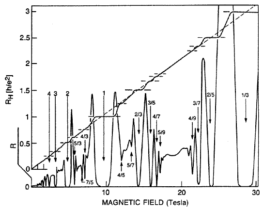
Figure 1.1: The longitudinal and transversal resistance in Hall bar as functions of the magnetic field. In the transversal resistance the plateaus of quantized values are evident. From [10].

The transversal resistance $\rho_{xy}$ of this system shows an exact quantization in its dependence on the magnetic field, $\rho_{xy}=h/e^{2}\nu$ with $\nu$ an integer or rational. The longitudinal resistance $\rho_{xx}$, on the other hand, shows a very non trivial behavior, vanishing or having a delta-like behavior when the transversal conductance resides on a plateau or passes through two distinct plateaus, respectively, (see for reference Fig. 1.1). The QHE can be expressed hence by the relations

$$\begin{split}{\bf j}=&\hat{\sigma}{\bf E},\\ \hat{\sigma}=&\frac{e^{2}\nu}{h}\left(\begin{array}[]{cc}0&1\\ -1&0\end{array}\right).\end{split}$$ (1.1)

The first equation is the Ohm’s law in matrix form and relates the current density to the electric field in the material. In the plateau regions the conductivity matrix becomes purely off-diagonal and is expressed in terms of a universal conductance quantum ($e^{2}/h$) and of a number $\nu$. From the experiments we know that $\nu$, which takes the name of filling fraction, assumes only integer and fractional values. We separate the case when $\nu$ is an integer, and call this phase Integer Quantum Hall Effect (IQHE), or a fractional number, namely the Fractional Quantum Hall Effect (FQHE).

It is widely believed that the IQHE and FQHE have a very different physical origin. IQHE is thought to come from the interplay between the Landau Levels quantization of the motion of a charged particle in a magnetic field, and the disorder. FQHE cannot be explained without taking into account the electron-electron interaction. This leads to a new state of matter in which one may have a new kind of quasi-particles carring a fractional charge [3]. A hierarchy of fractional filling fractions was justified theoretically by assuming that in the FQHE the quasi-particles which consistute the excitation of the system can undergo a IQHE. The idea is that every quasi-particle carries a number of magnetic flux quanta which partially compensates for the external magnetic field. Hence the quasi-particles may give rise to a IQHE phase when the effective magnetic field, obtained as the difference of the external applied field and the sum of the magnetic fields attached to the quasi-particles, assumes certain values [8].

The quasi-particles defined in these theoretical approaches belong to the bulk of the system. However it was showed that the current in the QHE is concentrated on the edges of the system [11]. This can be justified by a semiclassical approach. The finite size of the sample can be taken into account by an external potential which bends up near the physical edges. The electrons that are well inside the system bulk move on circular orbits whose radius is determined by the magnetic field. Hence they are fully localized and cannot contribute to the transport. However the orbit of the electrons which reside near one edge is not fully contained in the system. From a classical point of view these electrons are reflected by the barrier generated by the confining potential and they propagate all in the same direction because the magnetic field fixes the sign of the circulation. Then there is the possibility of the formation of ‘skipping orbits’ which can travel through the system. From a quantal point of view the electrons localized near the edge of the system reside in the ‘edge states’ whose properties we will discuss in the following.

In this thesis we will be concerned with transport properties and edge dynamics in the FQHE regime. We will show that the charged excitations of a two-dimensional electron liquid are concentrated in the edges of the systems thereby forming a one-dimensional system. Hence we can study the transport properties of the whole system by studying the interaction beetween two one-dimensional systems. It is believed that the edges of a system in the FQHE regime are a nearly perfect realization of the (Chiral) Luttinger Liquid ($\chi$LL)[12, 13]. The Luttinger Liquid model describes one-dimensional electron liquid with linear energy dispersion. It is an exactly solvable model and it will be a fundamental tool in this thesis. We will describe its basic properties in the following chapter.

Starting from some physical reasonable assumptions we will show that the localization of the density excitations in the region of the edges is independent of the presence of a developed QH phase. We will derive an equation of motion for such excitations and then use the solutions of this equation to calculate the electrical transport properties.

This research was stimulated by a collaboration with an experimental group. The main experimental aim was the realization of new electronic devices able to detect the fractionally charged quasi-particles. To this end, it was planned to study the transport through a constriction in the two-dimensional electron liquid. This kind of problems have been treated theoretically in the past by considering the constriction as a quantum point contact in the sense that in a very narrow region the edges of the Hall liquid come almost in contact so enhancing the probability of the tunneling of excitations between the edges [14, 15, 16]. In this thesis we will drop the assumption that the constriction has zero extension, and we will show that, by taking into account a finite size of the constriction, one obtains different results for the tunneling current. In particular, we may obtain a better qualitative agreement with the experimental results in certain ranges of temperature.

1.1 The Classical Hall effect

We will start our discussion of the QHE by recalling the Classical effect. The Classical Hall effect occurs when a current flows in a metal in the presence of a uniform magnetic field. The motion of a charged particle in a magnetic field can be separated in the motion parallel to the direction of the magnetic field and in the motion perpendicular to such direction. We assume that the magnetic field is parallel to the direction of the $\hat{z}$ axis

$${\vec{B}}=-B\hat{z}$$ (1.2)

and we choose a right handed set of orthogonal axis $(x,y,z)$. The equation of motion projected in the $\hat{z}$ direction is given by

$$\ddot{z}=-eE_{z}$$ (1.3)

hence the particle is uniformly accelerated in this direction.

We neglect in the following such motion and consider the particle confined in a two-dimensional plane $(x,y)$. The equation of motion can be written as

$$m\ddot{\bf r}=-e{\bf E}-e{\bf v}\times{\bf B}.$$ (1.4)

When we consider the equilibrium situation we have that the acceleration must be zero and we obtain

$${\bf J}=\hat{\sigma}{\bf E}$$ (1.5)

where we have defined the current density

$${\bf J}=-ne{\bf v},$$ (1.6)

and the conductivity matrix

$$\hat{\sigma}=\left(\begin{array}[]{cc}0&-\sigma_{H}\\ \sigma_{H}&0\end{array}\right).$$ (1.7)

The classical Hall resistance ($R_{H}$), defined by

$$\sigma_{H}=R_{H}^{-1}=\frac{ne}{B},$$ (1.8)

where $n$ is the electron number density, is then linearly dependent on the magnetic field.

The measure of the Hall resistance as a function of the magnetic field gives information on the electron density in metals. Notice that the Hall resistance is measured in the transversal direction with respect to the direction of the current. The conductivity matrix however is not complete. Indeed the Eqs. (1.5) and (1.7) imply that the longitudinal conductivity is zero. Hence the current in that direction will flow without dissipation. In fact the classical Hall effect and the usual metal dissipation must be considered together then giving the conductivity matrix for a metal in a magnetic field

$$\hat{\sigma}=\left(\begin{array}[]{cc}\sigma_{D}&-\sigma_{H}\\ \sigma_{H}&\sigma_{D}\end{array}\right)$$ (1.9)

where $\sigma_{D}$ is the Drude conductivity.

We can understand the classical Hall effect in the following way. When the magnetic field is zero the electron current flows following the gradient of the electric potential. If one turns on the magnetic field the motion of the particle becomes circular as one can easily verify be solving the equations of motion. The important point to stress is that the circulation is determined by the sign of the magnetic field and hence all the particles, which run in the same direction, turn in the same way. This effect creates a mean transversal current and a charge accumulation at one edge of the metal. To maintain the electrical neutrality an equal amount of opposite charges must accumulate at the other edge. This creates a transversal electrical field which will equilibrate the transversal current and establishes a dynamical equilibrium. The measure of the transversal electric field constitutes a way to measure the magnetic field.

We introduce now a relativistic notation which will become useful in the following. The electromagnetic field can be defined by using the vectorial and electric potentials $\vec{A}$ and $V$. In terms of these potentials the electric and magnetic fields are defined as

$$\begin{split}\vec{E}&=-\partial_{t}\vec{A}-\vec{\nabla}V,\\ \vec{B}&=\vec{\nabla}\times\vec{A}.\end{split}$$ (1.10)

We deal with only two spatial dimensions because, as we have seen, the problem can be separated and in the direction of the magnetic field the equation of motion is easily solved. On the other hand when we will address the quantum problem we will see that the particles are strongly confinated in the direction of the magnetic field and the problem can again be separated. We introduce the covariant “tri-vector” potential

$$A_{\mu}=(V,{\bf A})$$ (1.11)

where the index $\mu$ will run over $0,1,2$ with the convention that $0$ will coincide with the temporal part of the tri-vectors, $1$ coincides with the $x$ variable and $2$ with $y$. As an example the tri-derivative is

$$\partial_{\mu}=(\partial_{ct},-\partial_{x},-\partial_{y})=(\partial_{ct},-{\bf\nabla}).$$ (1.12)

We need to introduce also the metric

$$g_{\mu\nu}=\left(\begin{array}[]{ccc}1&0&0\\ 0&-1&0\\ 0&0&-1\end{array}\right),$$ (1.13)

and the totally antisymmetric Levi-Civita tensor $\epsilon_{\mu\nu}$. With these definitions, we may rewrite the magnetic and electric field in the form

$$\begin{split}E_{i}&=-\partial_{0}A_{i}+\partial_{i}A_{0}\\ B&=\epsilon_{jk}\partial^{j}A^{k}\end{split}$$ (1.14)

where, as usual in the relativistic notation, repeated indices are summed over. We can combine the equation (1.5) and the definition (1.8) in the compact form

$$J^{\mu}=\sigma_{H}\epsilon^{\mu}_{\phantom{\nu}\nu\lambda}\partial^{\nu}A^{\lambda}$$ (1.15)

where $J^{0}=c\rho=-ecn$. This equation is the phenonemological representantion of the Hall effect and it can be extended to the QHE because it comes directly from a Lorentz transformation which is valid if the system is translationally invariant. Its quantum counterpart constitutes the starting point for the seminal papers of Wen [14, 13, 17, 18] for the derivation of the properties of the FQHE. The main task of a microscopic theory of the QHE must be to derive this equation starting from a microscopic electron Hamiltonian.

1.2 A first glance to the Quantum Hall Effect

The classical theory of the Hall effect was well understood and proved very useful in the experimental characterization of the properties of non-magnetic metals. Hence the experimental result of von Klitzing et. al. [1], reported in Fig. 1.1, was totally unexpected.

Before discussing the features of this experimental result, let us consider briefly the experimental setup. The devices used in this type of experiments are semiconductor heterostructures or heterojunctions where the electron gas resides at the interface between two different semiconductor species. The polarization of the different semiconductors generates a uniform electric field which confines the electrons in a small region localized around the interface as it is indicated in Fig. 1.2.

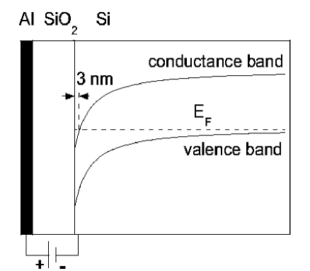
Figure 1.2: A simple scheme of the electron confinement around an interface between two different semiconductors.

Hence the electron gas can be considered as two-dimensional. This introduces a great simplification. Indeed it is well known that the resistivity $\rho$, and the resistance $R$ are related by

$$R=\rho L^{(2-d)}$$ (1.16)

where $d$ is the dimension of the system and in two dimensions these two quantities coincide.

We choose the direction of the electric field as the $\hat{z}$ axis. In this direction a magnetic field will be also applied. To reduce the thermal effects the device is maintained at temperatures below $1$ K (the newest experimental setups can reach about $10$ mK). The electron gas is contacted with a multiprobe setup. Two of these contacts are used to inject a steady-state current and two other contacts are used to measure the potential drop in the system. A six-probe setup is shown in Fig. 1.3.

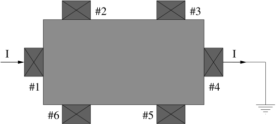
Figure 1.3: a) A schematic of the device used in the experiment on the Quantum Hall effect. The source ($\#1$) and drain ($\#4$) contacts are used to inject in the system a steady-state current $I$. The other probes ($\#2,\#3,\#5,\#6$) are used to measure the potential drop in the system to obtain the curves in Fig. 1.1.

Once the current is fixed we can measure the Hall resistance by measuring the voltage drop, as for instance, on the probe $4$ and $1$ or the longitudinal resistance by measuring the potential of the contacts $4$ and $3$ of the device in Fig 1.3. The results of these measurements at very high magnetic field and very low temperature are shown in Fig. 1.1. In that figure the longitudinal and transversal resistances are reported. By using the Eq. (1.8) for the Hall resistance and the Drude part for the longitudinal resistance one expects that the longitudinal resistance is a constant and the transversal is linearly dependent on the magnetic field intensity.

From the experimental data we see that this is not true (see Fig. 1.1). The transversal resistance shows clear and large plateaus. In these plateaus the resistance has a fixed value which is proportional to the quantum of conductance $e^{2}/h$ and the constant of proportionality is a integer or rational number. Outside the plateaus its relation with ${\bf B}$ becomes linear. More strange is the behavior of the longitudinal resistance. For small value of the magnetic field the Shubnikov-DeHaas oscillations are seen. However when the amplitude of these oscillations increases the longitudinal resistance shows an alternation of high maxima and flat regions where its value is zero. The plot shown in Fig. 1.1 is a more recent version of the combined result of von Klitzing [1] on IQHE and Stormer, Gossard and Tsui [2] on FQHE.

What is paradoxical in these results is that the electron-electron interactions and the disorder play a fundamental role to obtain it rather than destroy it. Indeed the results for the conductances in the previous section can be derived by using only the relativistic invariance [19], hence it does not matter if the system is classical or quantum and the electrons form a gas or a solid just maintaining the translational invariance.

Let us notice another peculiar aspect of this effect. In the region where the longitudinal resistivity is nearly zero and the transversal one is quantized, the system behaves like a superconductor ($\rho_{xx}=0$) and like an insulator ($\sigma_{xx}=0$). The reason for that is the presence of the finite off-diagonal terms, $\sigma_{xy}$, which assures the existence of the inverse of the matrix $\hat{\sigma}$ and the finite value of the $\rho_{xy}$ resistivity.

1.3 The Integer Quantum Hall Effect

Let us start the theoretical study of the QHE from the Integer Quantum Hall Effect, this being the first experimentally observed [1] and the more theoretically understood. In this effect the resistivity $\rho_{xy}$ is quantized in terms of the quantum $h/e^{2}$ and the costant of proportionality is an integer (measured with a precision of a part over $10^{8}$).

The very starting point is the quantum motion of a charged particle in a magnetic field. As it is well known, the motion of a charged particle in a magnetic field is obtained from the free Hamiltonian with the “minimal substitution”

$${\bf p}\to{\bf p}+e{\bf A}$$ (1.17)

where ${\bf A}$ is the vector potential. The presence of an electric potential does not affect such transformation and the Hamiltonian then reads

$$H=\frac{1}{2m}\left({\bf p}+e{\bf A}\right)^{2}-e\Phi.$$ (1.18)

We consider the simplest case of $\Phi\equiv 0$. There are many ways to solve the Schrödinger equation for a single particle. We consider here a field-theoretical inclined approach that will provide some useful relations to understand the modern literature. The position and momentum operators follow the usual commutation relations

$$\begin{split}&[x,p_{x}]=[y,p_{y}]=i\hbar,\\ &\mbox{others}=0.\end{split}$$ (1.19)

We define the new operators

$$\begin{split}&\xi=\frac{1}{eB}\left(p_{y}+eA_{y}\right),\\ &\eta=-\frac{1}{eB}\left(p_{x}+eA_{x}\right),\\ &X=x-\xi,\\ &Y=y-\eta,\end{split}$$ (1.20)

which follow the commutation relations

$$\begin{split}&[X,Y]=-[\eta,\xi]=-i\ell^{2},\\ &\mbox{others}=0,\end{split}$$ (1.21)

where we have introduced the magnetic length $\ell^{2}=\hbar/eB$. To obtain these commutation relations we must remember that $A_{x}$ and $A_{y}$ are in general function of both the operators $x$ and $y$. On the other hand, the rotor of ${\bf A}$ is independent from $x$ and $y$ and hence the vector potential must be a linear function of these operators and the commutators turn out to be c-numbers.

In terms of these new operators the Hamiltonian takes the simple form

$$H=\frac{m}{2}\omega_{c}^{2}(\xi^{2}+\eta^{2})$$ (1.22)

where we are faced with the problem of a one dimensional harmonic oscillator in the variables $\eta$ and $\xi$ so that the energy spectrum is written immediately as

$$E_{n}=\left(n+\frac{1}{2}\right)\hbar\omega_{c}$$ (1.23)

where we have introduced the ciclotron frequency $\omega_{c}=eB/m$. The energy levels take the name of “Landau Levels” (LL) after the solution of Landau of the motion of a particle in a magnetic field [20].

To obtain an explicit form for the eigenfunctions we must specify a gauge. A possible gauge is the Landau gauge

$${\bf A}=(By,0)$$ (1.24)

and we factorize the eigenfunction as

$$\psi(x,y)=\frac{e^{ik_{x}x}}{\sqrt{L}}\chi(y)$$ (1.25)

where $\chi$ is a solution of the Schrödinger equation

$$\left[-\frac{\hbar^{2}}{2m}\frac{d^{2}}{dy^{2}}+\frac{m}{2}\omega_{c}(k_{x}\ell^{2}-y)^{2}\right]\chi(y)=E_{n}\chi(y).$$ (1.26)

This is the Schrödinger equation of a harmonic oscillator with the center at $k_{x}\ell^{2}$ hence the solution is readily written in terms of a product of a gaussian and the Hermite polynomials. Notice that when evaluated over these functions the mean value of $Y$ depends only on $k_{x}$

$$\langle Y\rangle=k_{x}\ell^{2},$$ (1.27)

and because $Y$ does not depend on time we have that in this representation $Y=k_{x}\ell^{2}\hat{1}$.

Now let us turn on an electric field of amplitude $E_{y}$ in the $y$ direction. The electric field adds a term which is linear in $y$ hence when we substitute $y=\eta+Y$, we have a term linear in $\eta$ that changes the center of the harmonic oscillator and does not affect the energy, and a constant term in $Y$ which enters the energy

$$E_{n}(k_{x},E_{y})=\left(n+\frac{1}{2}\right)\hbar\omega_{c}+\frac{e^{2}E_{y}^{2}}{2m\omega_{c}^{2}}+eE_{y}\langle Y\rangle.$$ (1.28)

From this relation it is easy to calculate the velocities defined as

$${\bf v}=\frac{1}{\hbar}\frac{\partial E_{n}}{\partial{\bf k}}.$$ (1.29)

We have

$$\begin{split}&v_{x}=\frac{\ell^{2}}{\hbar}eE_{y},\\ &v_{y}=0\end{split}$$ (1.30)

and we can calculate the conductivity

$$\begin{split}&J_{x}=-env_{x}=-\frac{e^{2}\ell^{2}}{\hbar}nE_{y}=-\frac{e^{2}}{h}\nu E_{y}\\ &J_{y}=0\end{split}$$ (1.31)

where $n$ is the electron density ($N$ is the total number of electron) and we have defined the filling factor

$$\nu=\frac{n}{n_{B}}=\frac{N}{N_{B}}=\frac{hn}{eB}.$$ (1.32)

From the Eq. (1.31) one can directly compute the conductivity matrix as

$$\hat{\sigma}=\left(\begin{array}[]{cc}0&-e^{2}\nu/h\\ e^{2}\nu/h&0\end{array}\right).$$ (1.33)

In the definition of the filling factor (1.32) we have also defined the quantity $n_{B}=eB/h=(2\pi\ell^{2})^{-1}$. It is possible to relate this density to the degeneracy of the Landau levels. In fact let us consider the case of an infinite system which is constituted by the replication of a finite size, let us say $L_{x}\times L_{y}=S$, system. The quantum number $k_{x}$ must be quantized in this finite size system as $k_{x}=2\pi j/L_{x}$ and, on the other hand, the center of the electron orbit must be contained in such a system hence we have the upper limit $k_{x}\ell^{2}<L_{y}$. We see then that the discrete number $j$, which defines the quantization of $k_{x}$, must be limited by

$$j_{m}=\frac{L_{x}L_{y}}{2\pi\ell^{2}}=\frac{SB}{\frac{h}{e}}=\frac{\Phi}{\Phi_{0}}=N_{B}=n_{B}S.$$ (1.34)

Notice that this degeneracy is the same for every Landau level. From this relation we see that the quantity $N_{B}$ can be interpreted as the number of magnetic flux quanta contained in the system (we have used that $\Phi_{0}=h/e$ is the magnetic flux quantum). Hence the filling factor can be interpreted as the mean number of flux quanta carried by the single electron. On the other hand the filling factor gives information about how many Landau levels are filled, indeed every Landau level can contain, as maximum, $j_{m}$ electrons and directly from the definition we have $\nu=N/j_{m}$. This simple model seems to reproduce most of the physics of the IQHE (the form of the conductivity matrix, its dependence of the universal quantity $e^{2}/h$ …), however up to now the filling factor $\nu$ is a positive real number and there is no way to introduce a quantization of this quantity. To introduce a quantization of the filling factor we need to consider an open system, i.e. a system where the number of electrons is not fixed but may vary due to the presence of one or more reservoirs.

Before discussing this situation let us consider the case of the electron gas confined in a potential $V(y)$ which is almost flat at the center and bends up at the edge of the system. We also assume that this potential is smooth on the scale of the magnetic length. If we assume that the potential is translationally invariant in the $x$ direction we can again separate the variables in Schrödinger equation and look for a solution of the form

$$\Psi(x,y)=\frac{e^{ik_{x}x}}{\sqrt{L_{x}}}f_{k_{x}}(y)$$ (1.35)

where $f_{k}(y)$ will not be the solution of the harmonic oscillator. Because of the hypothesis that the potential varies smoothly with respect to the magnetic length scale the function $f_{k_{x}}$ is centered around $k_{x}\ell^{2}=Y_{k_{x}}$ and the energy $E$ will be again given by the kinetic energy plus a potential term given by $V(Y_{k_{x}})$. Hence the group velocities are given by

$${\bf v}=\frac{1}{\hbar}\frac{dE_{n}}{d{\bf k}}$$ (1.36)

and again the $v_{y}$ component will be zero. The energy will depend on the momentum $k_{x}$ only in the region of high variation of the potential $V$ hence the particle will have a non-zero $x$ velocity only if they are close to the edges of the system. This then defines two regions, the left and the right edge where the electrons move with opposite velocities (recall that the energy will decrease when entering the device, from the left, and increase when leaving the device to the right). The width of these regions depends on the variation of the potential: if the potential $V$ varies very sharply these regions are very small, while if $V$ varies smoothly they are very large.

An example of this behavior is the simple case when the potential $V(y)$ is infinite outside the physical edges of the device and constant inside (it may be also zero). Hence its gradient is concentrated only in two points. We are then faced with the problem of a particle in a high magnetic field confined in a finite region. In the Landau gauge this problem is mapped into the problem of a particle moving in a 1D well and subjected to the harmonic potential. This problem is exactly solvable in terms of special functions (the Kummer functions $M$ and $U$ ) [21] and the condition of the confinement gives a relation between the momentum $k_{x}$ and the energy $E_{n}(k_{x})$. On the other hand when the magnetic field is very large we can solve the problem in an approximate way. Indeed in this hypothesis the magnetic length $\ell$ will be very small and when the electron center $k_{x}\ell^{2}$ is far away from the boundaries the energy is simply given by the harmonic oscillator energy and the ground state energy is the corresponding lowest energy level of the harmonic oscillator. However if the electron center $k_{x}\ell^{2}$ is exactly at one boundary the electron wave function must have a node in that point and be zero outside the system. This will imply that the ground state for this case is the first excited state of the harmonic oscillator. We then see that the energy increases continuously when the electron center moves from the bulk region, far from the edges, towards the boundary regions, close to the edges. A similar behavior is verified when the confining potential is smoothly varying. What happens when many Landau levels are filled? We can apply the above idea to every Landau level separately (we suppose that the electrons are not interacting) and the result is simply that there will be two edge states for each Landau level.

Let us now consider the more realistic case of an open system, where two reservoirs with different chemical potentials can inject electrons in the gas. We choose to place the reservoirs along the $x$ direction. What is now the total current flowing in the system? Because the currents at the edges flow in different directions we have simply

$$I=\int\limits_{\mu_{L}}^{\mu_{R}}d\mu~{}ev_{x}g(\mu)$$ (1.37)

where

$$g(E)=\frac{1}{L}\frac{dj(E)}{dE}=\frac{1}{2\pi\ell^{2}}\frac{dY}{dE}$$ (1.38)

is the one-dimensional density of states and we have used the fact that $j$ is related to $k_{x}$ by $k_{x}=2\pi j/L$. We use the one-dimensional density of states because the electrons that are confinated at the edge are moving in one dimension only. By using the expression for the velocity one arrives directly to

$$I=\frac{e}{h}(\mu_{L}-\mu_{R}).$$ (1.39)

This current is the same for every Landau level hence the total current will be

$$I_{t}=NI=\frac{eN}{h}(\mu_{L}-\mu_{R})=\frac{e^{2}N}{h}(V_{L}-V_{R})$$ (1.40)

where $V_{i}$ is the potential of the $i$-th edge ($\mu_{i}=eV_{i}$). The integers $N$ count the number of Landau levels that are beyond the Fermi energy (we are assuming that the chemical potentials $\mu_{L}$ and $\mu_{R}$ are close enough to consider only the linear response regime). Now we can calculate the conductivity matrix. When the probes belong to the same edge the current is the same (there is not backscattering) and one obtains a zero longitudinal resistance. When the probes belong to different edges the current is given by (1.40). We then obtain

$$\hat{\sigma}=\left(\begin{array}[]{cc}0&-\frac{Ne^{2}}{h}\\ \frac{Ne^{2}}{h}&0\end{array}\right).$$ (1.41)

It is now possible to understand the nature of the plateaus. The reservoirs will define an energy reference (the Fermi energy) and moving the magnetic field will vary the frequency $\omega_{c}$ and the Landau level energy. Only the Landau levels that are below the Fermi energy can participate to the current and this defines the number $N$. When a new Landau level sinks below (or become greater than) the Fermi energy the number $N$ will increase (decrease) by $1$ and the conductance can vary only by integers. On the other hand there is a finite energy gap, given by $\hbar\omega_{c}$ between two different Landau Levels. This finite gap implies the finiteness extension of the Hall conductance plateaus.

What remains unexplained by this model is why when a new Landau level sinks below the Fermi energy the longitudinal conductance has a maximum and the Hall conductance shows a linear behavior. It is mostly believed that this behavior can be explained by inserting in the above model the effect of the disorder. The idea is that when a new Landau level crosses the Fermi level, a path which connects two edges may appear and this allows for the presence of backscattering and the longitudinal conductance is not zero. The connection between the two edges is created by the presence of the impurities that create localized islands and the electrons can, tunneling from one island to the other, be backscattered to the other edge. Numerical evidences of this percolation scheme have been provided but there is not an accepted model which reproduces the experimental data and allows us to understand completely this phenomenon.

1.4 The Fractional Quantum Hall Effect

The theory we have presented in the preceding section can explain the IQHE. However in the 1982 Tsui et al. showed that in cleaner sample and at higher magnetic field than that used by von Klitzing a new series of plateaus in the Hall resistance appears [2](see Fig. 1.1). These new plateaus appear when all the electrons are in the lowest Landau level, hence there is not the possibility that new edge states can be created when varying the magnetic field. Another obscure point is that the transversal conductance is again given by an expression similar to Eq. (1.41) but with the integer number $N$ substituted by a rational number. This rational number is identified with the filling fraction $\nu$. This effect is now widely known as Fractional Quantum Hall Effect.

There is not a complete accepted theory for this effect even though many theoretical ideas have been developed to understand its physics. A review of all these ideas is outside the scope of this thesis. However the interested reader can refer to some beautiful reviews [22, 23, 24, 9].

The first observation we can make in dealing with this effect is that the kinetic energy, since all the electrons reside in the LLL, is a constant and can be neglected. Hence the electron-electron interaction, which in the IQHE is treated as a perturbation, plays a fundamental role. If the interaction cannot be neglected the correlation between the particles must be taken into account in the search for the ground state. When we consider the problem of many electrons usually we first write the single particle wave function and then the many-particle wave function is given by a Slater determinant. However when the particles are strongly interacting this approach fails and we must write a wave-function which takes into account the correlation. On this track, Laughlin moved in the 1983 [3]. He wrote a trial wave function of the form

$$\psi=\prod_{i\not=j}(z_{i}-z_{j})^{m}\exp\left(-\sum_{i}\frac{|z_{i}|^{2}}{4\ell^{2}}\right),$$ (1.42)

where $m$ is an odd integer and $z_{j}=x_{j}+iy_{j}$ is a complex variable which describes the position of the $j-th$ particle. He proved by using numerical calculation that this wave-function minimizes the interaction energy. This minimization can be easily understood by observing that in the Laughlin wave-function the multiplicity of the zeros is greater than that of the fermion (this case is recovered by setting $m=1$). Laughlin was also able to show that the state described by this wave-function is incompressible, hence there is a gap in the energy spectrum. The presence of the gap is necessary to understand the finite extension of the plateaus as in the case of the IQHE.

Laughlin pointed out also that the quasi-particle excitations of this ground state have fractional charges given by $e/m$. The direct observation of such fractional charges has captured the major experimental efforts and was achieved in the 1997 by several experimental groups with different techniques [7, 25, 4].

The Laughlin’s proposal can explain the presence of the plateaus at filling fraction given by a rational number which is the inverse of an odd number. However a more recent theory extended the model capturing also a series of possible values of the filling fractions. The starting point of these theories was the pioneering work of Jain [8] which pointed out that the FQHE can be explained as the IQHE phase of the ground-state excitations. These quasi-particles, called Composite Fermions, carry a certain number of magnetic flux quanta per particle and see a residual magnetic field. Under certain conditions these fermions can develop a IQHE phase. With this idea Jain was able to predict a series of filling fraction given by

$$\nu=\frac{p}{pm\pm 1}$$ (1.43)

where $p$ is an odd integer and $m$ is an integer.

An earlier approach to the generalization of the allowed values of $\nu$ is the hierarchical approach developed by Haldane [26] and Halperin [27]. The general idea of this approach goes as follows. We consider a given FQHE state in its ground state. When we change the magnetic field we add quasi-particles to the system. These quasi-particles move in the magnetic field determined by the difference of the external magnetic field and the magnetic field carried by the particles which form the ground state. When we increase again the magnetic field the quasi-particles develop a new Quantum Hall phase. The new filling fraction is now given by a complex fraction composed by the integer numbers which identify the starting state and the new integer which identify the new developed phase. A complete review of these ideas can be found in Wen [18]. A major aspect of this theory is that a series of excitations starts to develop and a given filling fraction $\nu=m/p$ might be the result of many of these steps. This in turn implies that many modes can propagate in the system. This can be the basis to understand some recent experimental results [28, 5, 6]

A major shortcoming of this theory is that its starting point is the phenomenological relation (1.15) (see Ref. [18] and references therein) where the presence of a developed Quantum Hall phase has been assumed implicitely. Up to now, at the best of our knowledge, no one was able to derive this equation from the fundamental properties of the electrons in the magnetic field confined in a finite size device. Even in the Composite Fermions approach, one of the most widely used theories to study the FQHE, it is not clear how to derive, starting from the correlated wave function, the presence of a gap which can justify the quantization of the Hall conductance.

1.5 Edge dynamics

In a series of beautiful papers Wen shows that the edge dynamics can be described by using a so called Chiral Luttinger Liquid ($\chi$LL) [13, 17, 14]. We want to discuss briefly this theory without entering in the details. In the following chapters we will compare this theory with our model.

The Wen’s starting point is the phenomenological equation (1.15). This equation is the requirement that a QHE is fully developed and we are in one of the plateau of the Hall conductance. It relates the response of the system (the current $J^{\mu}$) to the external perturbation (the potential $A^{\mu}$) in a non-trivial way. We can define a Chern-Simons field $a^{\mu}$ by

$$J^{\mu}=\sigma_{H}\epsilon^{\mu}_{\phantom{\nu}\nu\lambda}\partial^{\nu}a^{\lambda}$$ (1.44)

and obtain the Eq. (1.15) as the equation of motion of the density lagrangian

$${\cal L}=\frac{\nu e^{2}}{2h}\epsilon^{\mu\lambda\eta}\tilde{A}_{\mu}\partial_{\lambda}\tilde{A}_{\eta}.$$ (1.45)

where $\tilde{A}_{\mu}=a_{\mu}-A_{\mu}$ and $a_{\mu}$ is the dynamical field.

As one can easily verify this lagrangian is not invariant with respect to a gauge transformation in a space with boundaries. To make the action gauge invariant Wen assumes that the lagrangian is written for the bulk operators and does not take into account the effects of the edges. Taking into account this contribution adds a term whose form can be derived from the gauge invariance and can be expressed in terms of current-current correlation functions. Wen was also able to show by assuming the locality of the theory that the excitations must have a gapless and linear spectrum. In particular, if one defines the current in the momentum space

$$J_{k}^{\alpha}=\int d\sigma\frac{1}{\sqrt{L}}e^{ik\sigma}J^{\alpha}(\sigma),$$ (1.46)

where $\alpha=(0,1)$ indicates the temporal ($0$) or spatial ($1$) component of the current vector and $\sigma$ parameterizes the boundary, then one gets

$$\begin{split}&[H,J_{k}^{\alpha}]=ckJ_{k}^{\alpha},\\ &[J_{k}^{+},J_{k^{\prime}}^{+}]=\frac{\nu e^{2}}{h}\delta_{k+k^{\prime},0},\\ &[J_{k}^{+},J_{k^{\prime}}^{-}]=[J_{k}^{-},J_{k^{\prime}}^{-}]=0,\end{split}$$ (1.47)

where by definition $J^{\pm}=1/2(J^{0}\pm J^{\sigma}/c)$. In these equations we have assumed that $c$ is the velocity of the boundary excitations and that they are chiral waves. From these equations it is also easy to show that the density fluctuations localized at the edge follow the commutation rules

$$[J_{k}^{0},J_{k^{\prime}}^{0}]=\frac{\nu e^{2}}{h}\delta_{k+k^{\prime},0}.$$ (1.48)

Wen now shows that one can “bosonize” the theory. The bosonization technique is a powerful idea to solve the problem of interacting one-dimensional electrons model or Tomonaga-Luttinger model. The main observation is that in the low-energy regime, the densities of a one dimensional electron system are boson operators. Hence instead of solving the problem for many interacting electrons with fermion properties one can solve the problem of the density modes which have bosonic properties [12].

We define a boson field $\phi$ with density lagrangian

$${\cal L}=\frac{1}{2}[(\partial_{0}\phi)^{2}-(\partial_{\sigma}\phi)^{2}]$$ (1.49)

and we require that this field is chiral, i.e. it satisfies the constraint

$$(\partial_{0}-\partial_{\sigma})\phi=0.$$ (1.50)

The equation of motion for this field is

$$(\partial_{0}-\partial_{\sigma})(\partial_{0}+\partial_{\sigma})\phi=0$$ (1.51)

which can be solved by assuming that

$$\phi=\phi_{0}+\tilde{\phi}_{0}+p_{\phi}(t+\sigma)+\tilde{p}_{\phi}(t-\sigma)+\sum_{n\not=0}\frac{1}{n}\left(\alpha_{n}e^{-in(t-\sigma)}+\tilde{\alpha}_{n}e^{-in(t+\sigma)}\right)$$ (1.52)

where $\phi_{0},~{}\tilde{\phi}_{0},~{}p_{\phi}$, and $\tilde{p}_{\phi}$ define the zero wavelength mode. The conjugate momentum

$$\pi=\frac{\delta{\cal L}}{\delta\partial_{0}\phi}=\partial_{0}\phi=p_{\phi}+\tilde{p}_{\phi}+\sum_{n\not=0}\left(\alpha_{n}e^{-in(t-\sigma)}+\tilde{\alpha}_{n}e^{-in(t+\sigma)}\right)=\phi_{L}+\phi_{R}$$ (1.53)

must satisfy the commutation rule $[\phi,\pi]=1$ hence we can derive the commutation rules of the operators in the expansion for $\phi$

$$\begin{split}&[\alpha_{n},\alpha_{n}]=[\tilde{\alpha}_{n},\tilde{\alpha}_{m}]=n\delta_{n,-m},\\ &[\phi_{0},p_{\phi}]=[\tilde{\phi}_{0},\tilde{p}_{\phi}]=i,\\ &\mbox{others}=0.\end{split}$$ (1.54)

It is possible to use the chirality condition to eliminate the field $\tilde{\phi}$, $\tilde{p}_{\phi}$ and $\tilde{\alpha}_{n}$. The hamiltonian is diagonalized

$$H=\frac{1}{2}p_{\phi}^{2}+\sum_{n>0}\alpha_{n}^{\dagger}\alpha_{n}$$ (1.55)

where we have neglected the constant terms.

By defining

$$J^{\alpha}=\frac{\sqrt{\nu}}{2\pi}\epsilon^{\alpha\beta}\partial_{\beta}\phi_{L},$$ (1.56)

where $\phi_{L}$ denotes the modes which satisfy the chirality condition, we can verify, starting from the boson algebra, that these operators satisfy the algebra of the edge excitation. Hence we have obtained a boson representation for the density fluctuations operators. To fully define all the algebra we need also the operators for the quasi-particles. Indeed the density $J^{\alpha}$ describes the edge density fluctuation with respect to an equilibrium density $\rho_{0}$. We look for an operator that can change such equilibrium density. To obtain a form for this operator we define the equilibrium charge

$$Q=e\int d\sigma J^{0}(\sigma)$$ (1.57)

and the quasi-particle operator

$$[\Psi,Q]=e^{*}\Psi$$ (1.58)

where $e^{*}$ can be different fron the electron charge. In fact in a physical system the quantum charge is the electron charge. However, here, we are postulating that the quasi-particle charge may not be the electron charge. We have seen in the preceding section that the “charge fractionalization” is useful to understand the phenomenology of the FQHE.

In the chiral boson theory the charged operators have a form

$$\Psi=:e^{i\gamma\phi_{L}}:$$ (1.59)

where the symbol $:\ldots:$ denotes the normal ordering and $\gamma$ is a constant. This constant can be determined by the commutation relation (1.58) by using the boson commutators (1.54) obtaining

$$\gamma=\frac{e^{*}}{e}\frac{1}{\sqrt{\nu}}.$$ (1.60)

Require that the operator $\Psi^{\dagger}$ creates a unitary charge corresponds to choose $\gamma\sqrt{\nu}=1$. The other requirememt that one can make is that the operator $\Psi$ satisfies the usual fermion (anti-)commutation relations. By using the Haussdorf lemma

$$e^{A}e^{B}=e^{[A,B]}e^{B}e^{A}$$ (1.61)

we obtain $\gamma^{2}=1/\nu={\rm odd~{}integer}$. Notice that this last relation says to us that if the condition $\nu=1/{\rm odd~{}integer}$ is not fulfilled hence the fermion creation operator must be composed by many different branches.

One can now calculate the fermion correlation function $G$ defined as

$$G=\langle\Psi^{\dagger}(t,\sigma)\Psi(0,0)\rangle.$$ (1.62)

By using again the Haussdorf lemma we obtain, in the limit of large system size, $\sigma/L\ll 1$

$$G=\left(\frac{i}{t+\sigma}\right)^{\frac{1}{\nu}}.$$ (1.63)

1.6 Transport through a constriction

It is possible to use the formulation for the edge dynamics we have depicted in the preceding sections to understand the effect of tunneling between the edges [14]. Such a phenomenon is present when two edges are close enough to have a non zero superposition of the quasi-particle wavefunction. The inclusion of tunneling in the edge model is done “by hand” in the sense that there is not a completely accepted model to derive the tunneling amplitude $\Gamma$ from the electron or quasi-particle properties. In the hamiltonian for the edges we then add a term proportional to the product of two distinct quasi-particle operators

$$H_{T}=\Gamma\Psi_{L}^{\dagger}\Psi_{R}+\Gamma^{*}\Psi_{R}^{\dagger}\Psi_{L}.$$ (1.64)

In the framework of the linear response theory one can calculate the tunneling current and the tunneling conductance which changes the Hall conductance in a non-universal way. The result of this approach is a non linear behavior of the current as a function of the tunneling voltage, the bias difference between the edges, i.e. the Hall voltage, and of the temperature [14]. In particular Wen obtained that

$$I\propto V^{\alpha-1}$$ (1.65)

where $\alpha=2/\nu$. A similar relation holds for the temperature dependence of the tunneling current

$$I\propto T^{\alpha-1}.$$ (1.66)

These relations stem directly from the power-law behavior of the correlation function $G$ of the quasi-particle.

The non-linear relation between the current and tunneling voltage are expected also for the Luttinger liquid model [12]. However the intrinsic difficulties in obtaining a very clean one-dimensional electron liquid reduce the possibility of the experimental observation of these results. In this sense the Wen’s papers open the possibility of a verification of these result on the edge of a quantum Hall liquid which, as we have briefly discussed, forms a very clean one-dimensional Luttinger liquid.

Similar results were extended later by Kane and Fisher, by using a Renormalization Group (RG) approach, to the effect of the impurity which mediates the tunneling [16]. In particular, they showed that any impurity between two edges under the RG analysis implies a strong coupling i.e. the edges will eventually close, the tunneling current diverges and the Hall bar separates in two distinct regions (this phenomenon is known as “overlap catastrophe”).

In this thesis we will generalize this approach in many ways. The first point we want to make is the generalization of the approach to the edge dynamics eliminating the limitation of incompressibility of the Hall liquid in the bulk. This is done by a hydrodynamical approach to the density fluctuation in the QHE and by the projection in the Lowest Landau Level. The projection on the LLL simplifies the Hamiltonian for the system quenching the kinetic energy but, on the other hand, introduces a non trivial quantum commutator between the density fluctuations and restores the full hardness of the problem. The hydrodynamical approach eliminates the fluctuations present at the scale of the magnetic length. This allows us to fully describe the system by using only the density fluctuations neglecting the real electrons and allows us to consider only the low energy excitations of the system. Similar approaches were used to study the tunneling of electron from a Fermi liquid to the edge of a fractional Quantum Hall liquid [29, 30].

On the other hand there are not conceptual difficulties in inserting in our model the intra- and inter-edge interactions. In this way we arrive to a problem similar to a Luttinger liquid model where an edge maps to a chiral branch of the liquid. However our edges are still interacting while in the Luttinger liquid model the reduction to chiral waves is done by eliminating the interactions.

The scheme we have depicted before and that we will discuss in the following brings us to the Hamiltonian for the density fluctuations. We bosonize these fields and obtain an equation of motion for the amplitude of the fluctuations. We choose a situable form of the intra- and inter-edge interaction and solve the equation of motion in many different edges profiles. In particular we are interested to the case when a constriction, which brings the edges to stay close, is present. It is possible to solve this case by using a scattering approach, i.e by defining the transmission and reflection coefficients for the wave which impinges on the constriction. We will show that the constriction does not change the low frequency (long wavelength) behavior of the conductance thus recovering the linear relation between the Hall conductance and the filling factor. To fully understand some new experimental results [28] we will introduce the tunneling between the edges. We restrict the tunneling only to the region of the constriction, hence we use the quasi-particle operators that are given by the solution of the equation of motion when the constriction is present. We develop a perturbative approach starting from the equation of motion for our operators and use it to calculate the tunneling conductance. This quantity, which modifies the Hall conductance, is a non linear function of the tunneling voltage and of the temperature as shown by Wen[14]. However the constriction introduces an energy scale. The characteristic time $t_{0}$ is given by the time that an edge excitation needs to travel through the constriction. This time introduces the energy scale $h/t_{0}$. We will show that the response functions of the system have different behaviors if the energy is above or below this energy threshold and this will affect the tunneling resistance.

Recent experimental results, reported by Roddaro et al. [28], show that the tunneling conductance for low bias voltage has a different behavior when compared with the Wen’s results. In particular they report that in their experimental setup at relatively high temperature the conductance shows a large maximum for zero bias voltage and two deep minima when the voltage is increased. When the temperature is lowered two main aspects appear. The zero bias maximum initially start to increase as expected but beyond a temperature near about $400~{}\rm{mK}$ the conductance starts to develop a large zero bias minimum. Beyond this temperature also a strong asymmetry starts to appear. From the discussion with the experimentalist we known that the appearance of the central deep in the conductance is not related to the presence of localized impurities.

Our model seems to capture some of the aspects of these results. In particular the presence of the deep minima seems to be related to the presence of the constriction and the comparison with the experiments can give information on $t_{0}$ and $e^{*}$. We predict also the presence of small oscillations on the tunneling resistance at large bias. The frequency of these oscillations is given by

$$\Delta V_{T}=\frac{h}{e^{*}t_{0}}=\frac{hc_{1}\cosh 2\theta_{1}}{e^{*}d\cosh 2\theta_{2}}$$ (1.67)

where $c_{1}$ is the velocity of the modes out of the constriction and $\theta_{1}$ and $\theta_{2}$ are related to the intra- and inter- edge interactions inside and outside the constriction.

The thesis is organized as follows. In this first chapter we have discussed the general phenomenology of the QHE and the Luttinger Liquid model. To do that we moved from the Classical Hall effect, given a look to the main experimental results of von Klitzing [1] and Tsui, Stormer, and Gossard [2] and discussed the theoretical result for the IQHE and the FQHE. We have also briefly reviewed the Wen’s theory for the edge dynamics and then discussed our main results.

In the second chapter we will concentrate on the derivation of our model and of the equation of motions. We will discuss its properties in the Hilbert space and solve the equation of motion in some simple cases that will prove to be useful in the following.

In the third chapter we will discuss the problem of defining and calculating the transport properties in these devices. We give a definition of the conductance and show how we recover, in the simple cases studied in the second chapter, the ideal Quantum Hall conductance.

In the fourth chapter we will abandon the limitations of a translational invariant system and discuss the presence of the tunneling between the edges. In this case we show that the tunneling gives a non-universal correction to the Quantum Hall conductance. We also compare our model with those present in the literature.

Finally, in the last chapter, we will discuss the comparison with some experimental results and the future perspectives of this research, and sumarize our main conclusions.

The results presented in this thesis have been submitted for pubblication in the Physical Review B journal. A preprint of this paper is available [31].

Chapter 2 The model for the Quantum Hall bar

We are interested in the study of a two-dimensional electron gas confined in a finite region in the presence of a high magnetic field. We will show that the description of the electron gas in terms of two interacting chiral Luttinger Liquid follows from some semi-classical assumptions we will discuss in the following. We want to point out also that we do not require that the system is in a Quantum Hall phase.

The ground state of the electron gas is characterized by a density $\rho_{0}({\bf r})$ which takes into account the electron-electron interaction and the action of the external potential which confines the system. We consider the excitations of this system as density fluctuations $\delta\rho({\bf r})$ near the “equilibrium” density $\rho_{0}({\bf r})$. The dynamics of these fluctuations is determined by the Hamiltonian

$$H=\frac{1}{2}\int d{\bf r}d{\bf r^{\prime}}~{}\delta\rho({\bf r})V({\bf r-r^{\prime}})\delta\rho({\bf r^{\prime}})$$ (2.1)

and by the commutation relations for the fields $\delta\rho$. In considering the Hamiltonian (2.1) we have projected all the operators in the lowest Landau level. Such a projection quenches the kinetic energy (it becomes simply a constant) but, as we will discuss later, introduces non-trivial commutation relations for the field $\delta\rho$.

In the definition of the Hamiltonian (see eq. (2.1)) we have inserted an interaction potential $V({\bf r-r^{\prime}})$ between two density fluctuations at different points. This electron-electron potential has a coulomb origin. In the following, however, we will assume a simple form for this potential.

2.1 The Luttinger Liquid model

In this section we will briefly review the solution of the Luttinger Liquid model because we will use a similar approach to the solution of our model and this analysis will be useful when we will compare our model with others present in the literature. We do not derive the Luttinger model starting from the physical properties of the interacting electrons in one dimension. The interested reader can refer to the seminal paper of Haldane [12] or to the book of Mahan [32].

The Luttinger Liquid model describes the dynamics of a one dimensional electron liquid. The Fermi surface of such a system is composed by two points $\pm k_{F}$ then with the same energy there are two species of excitations, the left and right movers defined by the sign of their momentum. We make the association $Left=L=+1$ and $Right=R=-1$. In the following we will consider also a spinorial notation where the upper component will be always related to the left movers.

When the electrons are not interacting the Hamiltonian operator is (we use $\hbar=c=1$)

$$H_{0}=v_{F}\int dx(\rho_{R}^{2}+\rho_{L}^{2})$$ (2.2)

where $v_{F}$ is the Fermi velocity and $\rho_{R}$ ($\rho_{L}$) is the density operator of the right (left) movers [12, 32] . The density operators follow the commutation relations

$$[\rho_{\alpha}(x),\rho_{\beta}(x^{\prime})]=-i\sigma_{\alpha,\beta}^{z}\partial_{x}\delta(x-x^{\prime}),$$ (2.3)

where $\alpha$ and $\beta$ assume the values $R$ or $L$. These relations can be derived by starting from the definition of the density operators in terms of the electron creation and annihilation operators and their anti-commutation rules.

It is customary to define the operators

$$\partial_{x}\theta_{\alpha}\equiv-\alpha\rho_{\alpha}.$$ (2.4)

These new operators will be useful in the following, when we will introduce the interaction, to diagonalize the total Hamiltonian. It easy to show that $\rho_{\alpha}$ and $\theta_{\alpha}$ are conjugate field

$$[\rho_{\alpha}(x),\theta_{\beta}(x^{\prime})]=-i\delta_{\alpha,\beta}\delta(x-x^{\prime}).$$ (2.5)

When we consider the interaction we add to the free Hamiltonian $H_{0}$ the term

$$\begin{split}H_{i}=&V_{1}\int dx(\rho_{R}^{2}+\rho_{L}^{2})+V_{2}\int dx(\rho_{R}\rho_{L}+\rho_{L}\rho_{R})\\ =&V_{1}\int dx((\partial_{x}\theta_{R})^{2}+(\partial_{x}\theta_{L})^{2})+V_{2}\int dx(\partial_{x}\theta_{R}\partial_{x}\theta_{L}+\partial_{x}\theta_{L}\partial_{x}\theta_{R})\end{split}$$ (2.6)

where $V_{1}$ and $V_{2}$ are the limit of vanishing momenta of the Coulomb interaction between the right and left movers. $V_{1}$ is the interaction between electrons that belong to the same species, while $V_{2}$ is the inter-species interaction. Notice that the interaction preserves the momentum.

The first step towards the solution of this problem is the diagonalization of the total Hamiltonian $H=H_{0}+H_{i}$. We can accomplish this task with the linear transformation

$$\begin{split}&\theta_{N}=\theta_{R}+\theta_{L},\\ &\theta_{J}=\theta_{R}-\theta_{L},\end{split}$$ (2.7)

and obtain the new Hamiltonian as

$$H=\frac{v}{2}\int dx\left[g(\partial_{x}\theta_{N})^{2}+\frac{1}{g}(\partial_{x}\theta_{J})^{2}\right]$$ (2.8)

where we have defined

$$\begin{split}v&=v_{F}\sqrt{\left(1+\frac{V_{1}}{v_{F}}\right)^{2}-\left(\frac{V_{2}}{v_{F}}\right)^{2}},\\ g&=\sqrt{\frac{v_{F}+V_{1}+V_{2}}{v_{F}+V_{1}-V_{2}}}.\end{split}$$ (2.9)

The Hamiltonian is separated but the new field $\theta_{N}$ and $\theta_{J}$ are conjugate fields, indeed their commutation relations are

$$[\partial_{x}\theta_{N}(x),\theta_{J}(x^{\prime})]=[\partial_{x}\theta_{J}(x),\theta_{N}(x^{\prime})]=-2i\delta(x-x^{\prime}).$$ (2.10)

Notice also that these fields are not chiral modes. The decomposition of the problem in terms of non-interacting chiral modes is not yet complete.

To obtain a set of independent fields we consider the new transformation on the fields $\theta_{N}$ and $\theta_{J}$

$$\begin{split}\phi_{R}=g\theta_{N}+\theta_{J},\\ \phi_{L}=g\theta_{N}-\theta_{J}.\end{split}$$ (2.11)

The Hamiltonian in terms of these fields is now

$$H=\frac{v}{8g}\int dx\left[(\partial_{x}\phi_{R})^{2}+(\partial_{x}\phi_{L})^{2}\right]$$ (2.12)

and we have

$$\left[\partial_{x}\phi_{\alpha}(x),\phi_{\beta}(x^{\prime})\right]=-4ig\sigma_{\alpha,\beta}^{z}\delta(x-x^{\prime}).$$ (2.13)

The equation of motion for the fields $\phi$ are

$$\begin{split}&\dot{\phi}_{R}=v\partial_{x}\phi_{R}\\ &\dot{\phi}_{L}=-v\partial_{x}\phi_{L}\end{split}$$ (2.14)

hence these modes are chiral.

We finally can express the density operator in terms of these chiral modes

$$\begin{split}\rho_{R}(x)=\frac{g+1}{4g}\partial_{x}\phi_{R}-\frac{g-1}{4g}\partial_{x}\phi_{L},\\ \rho_{L}(x)=\frac{g-1}{4g}\partial_{x}\phi_{R}-\frac{g+1}{4g}\partial_{x}\phi_{L},\end{split}$$ (2.15)

and obtain the total density operator $\rho=\rho_{R}+\rho_{L}$ as

$$\rho=\frac{1}{2}\partial_{x}(\phi_{R}-\phi_{L})=\frac{1}{2v}\partial_{t}(\phi_{R}+\phi_{L}).$$ (2.16)

The total current is defined by using the continuity equation $\dot{\rho}=-\partial_{x}I$ and then

$$I=-\frac{v}{2}\partial_{x}(\phi_{R}+\phi_{L})=-\frac{1}{2}\partial_{t}(\phi_{R}-\phi_{L}).$$ (2.17)

When we consider the chiral Luttinger liquid ($\chi$LL) we fix one of the fields $\phi$ to zero and consider the dynamics of the other field given by the Hamiltonian (2.12) and the commutation relation (2.13). Notice that we have started with two interacting chiral modes and after a non-canonical transformation we have obtained two non-interacting chiral modes with non-trivial commutation relation. As it is seen from Eq. (2.15), the chiral modes $\phi$ are a linear combination of the starting interacting chiral modes $\theta_{R}$ and $\theta_{L}$.

2.2 Lowest Landau level projection and the hydrodynamical approximation

The Hamiltonian (2.1) alone cannot determine the dynamics of the fields $\delta\rho$. To do that we need to give either the equation of motion or the commutation rules for these fields. To calculate the commutation relations we project all our field on to the lowest Landau Level. The theoretical approach to this projection and its physical implications are discussed in a more detailed way in many reviews or articles (see as an example Ref. [33]). In the following we will use it in fixing the wave functions of the single electron.

In order to emphasize the role of the two main physical approximations, i.e., the LLL projection and the hydrodynamical approximation, it is convenient to start from the second quantized form of the density fluctuation

$$\delta\hat{\rho}({\bf r})=\sum_{k\not=h}\hat{c}_{k}^{\dagger}\hat{c}_{h}\varphi_{k}^{*}({\bf r})\varphi_{h}({\bf r})$$ (2.18)

from which we have

$$\begin{split}[\delta\hat{\rho}({\bf r}),\delta\hat{\rho}({\bf r}^{\prime})]=&\sum_{k\not=h,m\not=l}\left(\hat{c}^{\dagger}_{k}\hat{c}_{l}\delta_{h,m}-\hat{c}^{\dagger}_{h}\hat{c}_{m}\delta_{k,l}\right)\\ &\times\varphi_{k}^{*}({\bf r})\varphi_{h}({\bf r})\varphi_{m}^{*}({\bf r}^{\prime})\varphi_{l}({\bf r}^{\prime}).\end{split}$$ (2.19)

The indices $k$ and $h$ in Eq.(2.18) label states in the LLL within the Landau gauge ${\bf A}=(By,0,0)$. The condition $k\neq h$ excludes the equilibrium contribution to the density $\rho_{0}({\bf r})$. In the spirit of the hydrodynamic approach, the latter is related to the ground state expectation value

$$\hat{c}^{\dagger}_{k}\hat{c}_{l}\to\langle\hat{c}^{\dagger}_{k}\hat{c}_{k}\rangle\delta_{k,l}=n(k)\delta_{k,l}$$ (2.20)

via

$$\rho_{0}(y)=\int\limits_{-\infty}^{\infty}\frac{dk}{2\pi}~{}\frac{n(k)}{\sqrt{\pi l^{2}}}\exp\left[-\frac{(y+kl^{2})^{2}}{l^{2}}\right].$$ (2.21)

Here $n(k)$ is the occupation number for the state with momentum $k$ and in the homogeneous case, $n(k)=n_{0}$, the evaluation of the gaussian integral gives

$$\rho_{0}=\frac{n_{0}}{2\pi l^{2}}\Rightarrow n_{0}=2\pi l^{2}\rho_{0}=\nu$$ (2.22)

where $\nu$ is the filling factor.

The commutator between two different density fluctuations can be derived from the well known result [33]

$$[\rho({\bf q}),\rho({\bf k})]=\left(e^{k^{*}q\ell^{2}/2}-e^{-kq^{*}\ell^{2}/2}\right)\rho(\bf{k+q}).$$ (2.23)

When we consider the long wavelength density fluctuation we expand to the leading order in $k\ell$ and $q\ell$ and transform to real space to obtain

$$[\rho({\bf r}),\rho({\bf r^{\prime}})]\simeq i\ell^{2}\epsilon_{ij}\partial_{i}\rho_{0}({\bf r})\partial_{j}\delta({\bf r-r^{\prime}}).$$ (2.24)

Notice that we have substituted the density operator $\rho$ with its equilibrium expectation value $\rho_{0}({\bf r})$. This approximation is justified as long as we are interested to the linear dynamics of small fluctuations about the equilibrium state.

From these commutation relations and from the Hamiltonian (2.1) we can derive the equation of motion of the density fluctuation

$$\partial_{t}\delta\rho({\bf r},t)=\ell^{2}(\partial_{i}\rho_{0}({\bf r}))\epsilon_{ij}\partial_{i}\int d{\bf r^{\prime}}V({\bf r},{\bf r^{\prime}})\delta\rho({\bf r^{\prime}},t).$$ (2.25)

By this equation it is evident that the density fluctuation are localized in the region of variation of the equilibrium density $\rho_{0}$. The regions of maximum variation of $\rho_{0}$ are located near the edges hence the density fluctuation are confined near the edges of the Hall bar. Because this model for the edge dynamics agrees with that we find considering the large magnetic field limit of the hydrodynamical Euler equations [34] we call our approach “hydrodynamical”.

Attached to a point of every edge we consider a local right handed system of coordinates where the variable $y$ indicates the region of variation of the equilibrium density. To be more precise we consider the device reported in the Fig. 2.1.

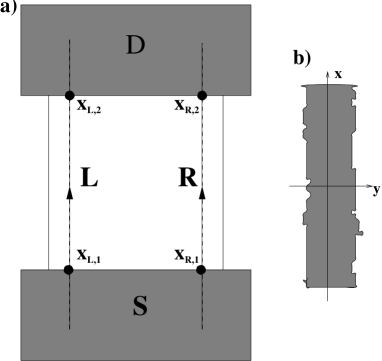
Figure 2.1: a) The scheme of a simple Quantum Hall bar contacted with two reservoirs. If we neglect the effect of the disorder, the edges runs parallels and translationally invariant along the $x$ direction. The $y$ axis is chosen to be orthogonal to the edges. b) A magnification of the edge region. We integrate with respect the $y$ direction to obtain a field varying only in the $x$ direction.

In this figure we draw a simple schematization of a Quantum Hall bar connected to two reservoirs (the drain (D) and the source (S)) bar where the physical edges are considered as parallels and translationally invariants. The coordinate $y$ is then orthogonal to the edge while the $x$ coordinate run along the edge.

The observation about the localization of the density fluctuation allows us to greatly simplify the problem. Indeed rather than solve the complete two-dimensional problem determined by the equation of motion (2.25), which implies the exact knowledge of the equilibrium density $\rho_{0}$ [34], we integrate over the $y$ direction, starting from the edge to well inside the bulk when we consider the fluctuation localized on the left edge and viceversa for the right edge, and obtain a one dimensional density fluctuation. In this way we define the operators

$$\delta\rho_{\alpha}(x)=\int\limits_{\alpha}dy~{}\delta\rho({\bf r})$$ (2.26)

where the index $\alpha$ identifies the edge to which the density fluctuation belongs. These new operators must satisfy the commutator law (2.24) when we integrate with respect to the $y$ and $y^{\prime}$ variables, following the prescription in (2.26). It is possible to show that the result of this operation is

$$[\delta\rho_{\alpha}(x),\delta\rho_{\beta}(x^{\prime})]=-i\frac{\nu(x)}{2\pi}\sigma_{\alpha,\beta}^{z}\partial_{x}\delta(x-x^{\prime}).$$ (2.27)

In the appendix A we give an alternative derivation of this equation starting directly from the operators $\delta\rho_{\alpha}$ in the case of sharp and smooth edges. We have also allowed for the possibility that the filling fraction $\nu$ is dependent on the position $x$ along the edge. In the following, for simplicity, we will drop this degree of freedom and consider a uniform filling fraction.

The Hamiltonian for the operators $\delta\rho_{\alpha}$ is derived from the Hamiltonian (2.1) by an integration. To do that we suppose that the interaction potential is slowly varying on the dimension of the edge i.e. we approximate

$$V({\bf r-r^{\prime}})\simeq V_{\alpha,\beta}(x,x^{\prime})$$ (2.28)

with

$$V_{\alpha,\beta}(x,x^{\prime})=V(x,y_{\alpha};x^{\prime},y_{\beta})$$ (2.29)

where we have allowed for the possibility that the two density fluctuations belong to different edges. With this approximation we get (repeated indexes are summed over)

$$H=\frac{1}{2}\int~{}dxdx^{\prime}~{}\delta\rho_{\alpha}(x)V_{\alpha,\beta}(x,x^{\prime})\delta\rho_{\beta}(x^{\prime}).$$ (2.30)

This Hamiltonian together with the commutation relations (2.27) determines the equation of motion for the $\delta\rho_{\alpha}$ operator

$$\partial_{t}\delta\rho_{\alpha}(x)=-\frac{\nu(x)\sigma_{\alpha,\beta}^{z}}{2\pi}\int\limits_{-\infty}^{\infty}dx^{\prime}\partial_{x}V_{\beta,\gamma}(x,x^{\prime})\delta\rho_{\gamma}(x^{\prime}).$$ (2.31)

This is our first major result. The solution of this equation describes the excitations of our system and will be the fundamental tool to obtain the response functions.

The commutation relations (2.27) when $\nu$ is constant are the reproduction of the Kac-Moody current algebra (2.13) for the density field in the $\chi$LL model. Notice however that our derivation of the $\chi$LL model has nothing to do with the QHE. Indeed it depends only on the high magnetic field limit (projection on the LLL) and on the coarse-graining (hydrodynamical approximation). Our derivation is therefore valid for every real value of the filling fraction whereas the QHE occurs only for certain value of $\nu$. We want to point out also that in our model every edge exhibits a $\chi$LL behavior even if the interactions are turned off, and that it is not possible to map the problem of two interacting QH edges to one Luttinger Liquid model.

2.3 The equation of motion

Let us now discuss the solutions of the equation of motion (2.31). To do that it is convenient to define the field $\phi_{\alpha}$ such that

$$\delta\rho_{\alpha}(x,t)=\partial_{x}\phi_{\alpha}(x,t).$$ (2.32)

These fields satisfy the commutation relations

$$[\phi_{\alpha}(x),\phi_{\beta}(x^{\prime})]=i\frac{\nu}{4\pi}\sigma_{\alpha,\beta}^{z}\mathrm{sign}(x-x^{\prime}).$$ (2.33)

In the following, we will consider also the function $\varphi_{\alpha}(x)$ which are the solutions of the equation

$$i\omega\sigma_{\alpha,\beta}^{z}\partial_{x}\varphi_{\beta}(x)=\frac{\nu}{2\pi}\int\limits_{-\infty}^{\infty}dx^{\prime}~{}\partial_{x}V_{\alpha,\beta}(x,x^{\prime})\partial_{x^{\prime}}\varphi_{\beta}(x^{\prime})$$ (2.34)

and we will show that the field $\phi_{\alpha}$ can be expressed in terms of the functions $\varphi_{\alpha}$ and the operators $b$ which turn out to have a Bose statistics.

To complete this task, we need to study the properties of the solutions of the equation (2.34). The first point we want to make is that these solutions form a complete and orthonormal basis of the Hilbert space. More precisely we will show that:

• all the frequencies $\omega_{n}$ are real and we label these states such that $\omega_{n}>0$ if and only if $n>0$;

• the eigenfunctions $\varphi_{n,\alpha}$ form a complete basis in the Hilbert space with the completeness relation

  $$\sum_{n}\mathrm{sign}(\omega_{n})\varphi_{n,\alpha}(x)\varphi^{*}_{n,\beta}(x^{\prime})\partial_{x^{\prime}_{\beta}}=\sigma_{\alpha,\beta}^{z}\delta(x-x^{\prime})$$ (2.35)

  and the orthonormality condition

  $$\sum_{\alpha}\sigma_{\alpha,\beta}^{z}\int dx~{}\varphi^{*}_{n,\alpha}(x)\partial_{x}\varphi_{m,\beta}(x)=\mathrm{sign}(\omega_{n})\delta_{n,m};$$ (2.36)

• the eigenfunction $\varphi_{n,\alpha}(x)$ is doubly degenerate.

The proof of these properties is detailed in the appendix B.

Having defined a basis for the Hilbert space we can develop the field $\phi_{\alpha}$ and $\delta\rho_{\alpha}$ in this basis. Indeed for every (spinorial) function $f_{\alpha}(x)$ we have

$$\begin{split}f_{\alpha}(x)=&\sum_{\beta}\int dx^{\prime}~{}\delta_{\beta,\alpha}\delta(x-x^{\prime})f_{\gamma}(x^{\prime})\\ =&\sum_{n}\varphi_{n,\alpha}(x)f(n)\end{split}$$ (2.37)

where we have defined

$$f(n)=-i\mathrm{sign}(\omega_{n})\int dx^{\prime}~{}\varphi_{n,\alpha}(x^{\prime})\sigma_{\alpha,\beta}^{z}\partial_{x^{\prime}}f_{\beta}(x^{\prime}).$$ (2.38)

This result implies that we can define the operator $\phi(n)$ as

$$\delta\rho_{\alpha}(x)=\sum_{n}\phi(n)\varphi_{n,\alpha}(x),$$ (2.39)

where $\phi(n)$ turns out to satisfy the commutation relation

$$[\phi(n),\phi^{\dagger}(n^{\prime})]=\frac{\nu}{2\pi}\mathrm{sign}(\omega_{n})\delta_{n,n^{\prime}},$$ (2.40)

and this suggests to define the operators $b$ such that

$$\phi(n)=\sqrt{\frac{\nu}{2\pi}}\left(b_{n}\theta(n)+b_{-n}^{\dagger}\theta(-n)\right).$$ (2.41)

It is easy to show that we have $[b_{n}^{\dagger},b_{n}]=1$ thus these operators follow the Bose statistics. We have then proved that we can expand the $\delta\rho_{\alpha}$ operator as

$$\delta\rho_{\alpha}(x)=\sqrt{\frac{\nu}{2\pi}}\sum_{n>0}\left(b_{n}\partial_{x}\varphi_{n,\alpha}(x)+b_{n}^{\dagger}\partial_{x}\varphi^{\dagger}_{n,\alpha}(x)\right)$$ (2.42)

and we obtain for the Hamiltonian

$$H=\sum_{n>0}\omega_{n}\left(b^{\dagger}_{n}b_{n}+\frac{1}{2}\right).$$ (2.43)

We define the current by starting from the continuity equation. The current in the edge $\alpha$ is, by definition, given by

$$\partial_{x}I_{\alpha}(x)=e\partial_{t}{\delta\rho_{\alpha}}(x)$$ (2.44)

and, up to a constant, we identify

$$I_{\alpha}(x)=e\partial_{t}\phi_{\alpha}(x).$$ (2.45)

We have then related all the quantities we want to calculate to the solutions of the equation of motion (2.34) and to the dynamics of the boson operators which is determined by the Hamiltonian (2.43).

2.4 Solutions of the equation of motion in simple cases

It is now instructive to solve the equation of motion for the function $\varphi_{\beta}$ is some simple cases, namely the case of two translationally invariant edges and when a constriction is present.

2.4.1 Translationally invariant case

The translationally invariant case is the simplest we can consider and we have for the potential the form

$$V_{\alpha,\beta}(x,x^{\prime})=V_{\alpha,\beta}(x-x^{\prime})=\left(\begin{array}[]{cc}V_{1}(x-x^{\prime})&V_{2}(x-x^{\prime})\\ V_{2}(x-x^{\prime})&V_{1}(x-x^{\prime})\end{array}\right)$$ (2.46)

where $V_{1}$ ($V_{2}$) is the intra-(inter-) edge interaction. We seek for the solution of the equation (2.34) in terms of plane waves, so we choose the form $\varphi_{\alpha}(x)=\varphi_{\alpha}(k)e^{ikx}$. This leads us to the $2\times 2$ eigenvalue problem

$$i\omega\left(\begin{array}[]{cc}1&0\\ 0&-1\end{array}\right)\left(\begin{array}[]{c}\varphi_{L}\\ \varphi_{R}\end{array}\right)=\frac{ik\nu}{2\pi}\left(\begin{array}[]{cc}V_{1}(k)&V_{2}(k)\\ V_{2}(k)&V_{1}(k)\end{array}\right)\left(\begin{array}[]{c}\varphi_{L}\\ \varphi_{R}\end{array}\right),$$ (2.47)

where $V_{1}(k)$ and $V_{2}(k)$ are the Fourier transform of $V_{1}(x)$ and $V_{2}(x)$ respectively. The eigenvalues are given by

$$\omega_{k}=\pm|k|\frac{\nu}{2\pi}\sqrt{V_{1}^{2}(k)-V_{2}^{2}(k)}=\pm c|k|$$ (2.48)

where $c$ is the sound velocity. Notice that for each positive frequency there are two counterpropagating modes: the “up-moving” solution is

$$\varphi^{u}_{k,\alpha}(x)=\frac{e^{ikx}}{\sqrt{kL}}\left(\begin{array}[]{c}u_{k}\\ -v_{k}\end{array}\right)$$ (2.49)

and the “down-moving” solution is

$$\varphi^{d}_{k,\alpha}(x)=\frac{e^{-ikx}}{\sqrt{kL}}\left(\begin{array}[]{c}v_{k}\\ -u_{k}\end{array}\right).$$ (2.50)

In these expression we have assumed $k>0$ and we have introduced the edge length $L$. This length is assumed to be arbitrary large (as usual when dealing with plane-wave) and will not enter the physical results. On the other hand the presence of the factor $1\sqrt{k}$ is imposed by the orthonormality condition. The orthonormality condition also fixes $u_{k}^{2}-v_{k}^{2}=1$ hence we can parameterize

$$\begin{split}u_{k}=\cosh(\theta_{k}),\\ v_{k}=\sinh(\theta_{k}),\end{split}$$ (2.51)

where the “mixing angle” $\theta_{k}$ is given by

$$\tanh 2\theta_{k}=\frac{V_{2}(k)}{V_{1}(k)}.$$ (2.52)

Let us discuss briefly these results. If we have two parallel non-interacting edges we have $\theta_{k}\equiv 0$ for every $k$ thus $u_{k}\equiv 1$ and $v_{k}\equiv 0$. This implies that the “up-moving” modes are fully concentrated on the left edge while the “down-moving” modes are concentrated only on the right. In this sense the left and right modes are well defined concepts and a good basis to discuss the properties of the system. Moreover we have a linear energy spectrum of these excitations with the edge velocity determined by the intra-edge interaction.

When the edges are interacting the modes propagates both on the left and on the right edge. The concept of left edge mode is ill-defined and the good basis in this case is the up-moving and down-moving modes. We will show, when discussing the transport, that the presence of the inter-edge interaction will not change the linear relation between the conductance and the filling fraction $\nu$ when one consider the limit of low-energy (which corresponds to the limit $k\to 0$) excitation. We want also point out that we have recovered the standard expression for the dispersion of the edge waves in the ordinary (non-chiral) Luttinger liquid model and that the $\chi$LL persists even if the interaction potential $V_{2}$ is turned off. This is due to the anomalous commutation relation (2.27) between the density fluctuations on the same edge.

2.4.2 A conservation law

At this point it is interesting to discuss the existence of a conserved quantity for the equation of motion (2.34). We assume for the interaction potential the form $V_{\alpha,\beta}(x-x^{\prime})=V_{\alpha,\beta}(x)\delta(x-x^{\prime})$. It is now possible to show that the quantity

$$\phi_{\alpha}^{\dagger}(x)\sigma_{\alpha,\beta}^{z}\phi_{\beta}(x)=\phi_{L}^{\dagger}(x)\phi_{L}(x)-\phi_{R}^{\dagger}(x)\phi_{R}(x)$$ (2.53)

is conserved

$$\partial_{x}\left(\phi_{\alpha}^{\dagger}(x)\sigma_{\alpha,\beta}^{z}\phi_{\beta}(x)\right)=0.$$ (2.54)

The proof of the existence of this conservation law rests on the assumption of the existence of the $V_{\alpha,\beta}$ matrix inverse for every value of $x$. Within this assumption, we can consider the equation of motions for the field $\phi_{\alpha}$ and its complex conjugate

$$\begin{split}i\omega\phi_{\alpha}(x)&=\frac{\nu}{2\pi}\sigma_{\alpha,\beta}^{z}V_{\beta,\gamma}(x)\partial_{x}\phi_{\gamma}(x),\\ -i\omega\phi_{\alpha}^{\dagger}(x)&=\frac{\nu}{2\pi}\partial_{x}\phi_{\gamma}^{\dagger}(x)V_{\gamma,\beta}(x)\sigma^{z}_{\beta,\alpha}.\end{split}$$ (2.55)

By taking the matrix $V_{\alpha,\beta}$ to the left-hand side of these equations and then multiplying the first (second) equation on the left (right) by $\phi_{\beta}^{\dagger}\sigma^{z}_{\beta,\alpha}$ ($\sigma_{\alpha,\beta}^{z}\phi_{\alpha}$) and summing the results we obtain the conservation law. Notice that, because $\phi_{\alpha}$ and $\varphi_{\alpha}$ follow the same equation of motion, this conservation law must be verified also by $\varphi_{\alpha}$.

The physical interpretation of this conservation law is interesting. It is possible to connect this law with the continuity equation and the conservation of the total charge and current. We have defined the current using the continuity equation and up to a constant we have

$$I_{\alpha}(x)=-ie\omega\phi_{\alpha}(x)$$ (2.56)

and we can express (2.54) in the form

$$\begin{split}0&=\partial_{x}\frac{1}{e^{2}\omega^{2}}\left(I_{L}^{2}(x)-I_{R}^{2}(x)\right).\end{split}$$ (2.57)

To appreciate the meaning of the above conservation law, let us consider the solution of the equation of motion. For simplicity we consider the translationally invariant case. The left and right density fluctuations are given by

$$\begin{split}\delta\rho_{L}(x)&=-ie\sum_{q>0}\sqrt{\frac{\nu}{2\pi q}}q\left[e^{iqx}\left(ub_{u,q}-vb_{d,q}^{\dagger}\right)-e^{-iqx}\left(-vb_{d,q}+ub_{u,q}^{\dagger}\right)\right],\\ \delta\rho_{R}(x)&=-ie\sum_{q>0}\sqrt{\frac{\nu}{2\pi q}}q\left[e^{iqx}\left(-vb_{u,q}+ub_{d,q}^{\dagger}\right)-e^{-iqx}\left(ub_{d,q}-vb_{u,q}^{\dagger}\right)\right]\end{split}$$ (2.58)

and the currents ($cq=\omega_{q}$)

$$\begin{split}I_{L}(x)&=-iec\sum_{q>0}\sqrt{\frac{\nu}{2\pi q}}q\left[e^{iqx}\left(ub_{u,q}+vb_{d,q}^{\dagger}\right)-e^{-iqx}\left(vb_{d,q}+ub_{u,q}^{\dagger}\right)\right],\\ I_{R}(x)&=-iec\sum_{q>0}\sqrt{\frac{\nu}{2\pi q}}q\left[-e^{iqx}\left(ub_{u,q}+vb_{d,q}^{\dagger}\right)+e^{-iqx}\left(vb_{d,q}+ub_{u,q}^{\dagger}\right)\right].\end{split}$$ (2.59)

Now we define

$$\delta\rho_{u}(x)=-ie\sum_{q>0}\sqrt{\frac{\nu}{2\pi q}}q\left[e^{iqx}b_{u,q}-e^{-iqx}b_{u,q}^{\dagger}\right],$$ (2.60)

$$\delta\rho_{d}(x)=-ie\sum_{q>0}\sqrt{\frac{\nu}{2\pi q}}q\left[e^{iqx}b_{d,q}^{\dagger}-e^{-iqx}b_{d,q}\right]$$ (2.61)

for the up and down moving fluctuations densities and again from the continuity equation

$$I_{u}(x)=-iec\sum_{q>0}\sqrt{\frac{\nu}{2\pi q}}q\left[e^{iqx}b_{u,q}-e^{-iqx}b_{u,q}^{\dagger}\right],$$ (2.62)

$$I_{d}(x)=-iec\sum_{q>0}\sqrt{\frac{\nu}{2\pi q}}q\left[e^{iqx}b_{d,q}^{\dagger}-e^{-iqx}b_{d,q}\right].$$ (2.63)

In terms of the up and down moving density fluctuations we have the simple relations

$$c(\delta\rho_{u}+\delta\rho_{d})=c\delta\rho=I_{u}-I_{d},$$ (2.64)

$$c(\delta\rho_{u}-\delta\rho_{d})=I_{u}+I_{d}=I,$$ (2.65)

so that the conservation of the total charge and the total current also implies the conservation of the product

$$(I_{u}-I_{d})(I_{u}+I_{d}).$$ (2.66)

Next we observe that

$$\delta\rho_{L}(x)=u\delta\rho_{u}(x)-v\delta\rho_{d}(x),$$ (2.67)

$$\delta\rho_{R}(x)=u\delta\rho_{d}(x)-v\delta\rho_{u}(x),$$ (2.68)

and

$$\left(\begin{array}[]{l}I_{L}(x)\\ I_{R}(x)\end{array}\right)=\left(\begin{array}[]{cc}u&-v\\ -v&u\end{array}\right)\left(\begin{array}[]{l}I_{u}(x)\\ I_{d}(x)\end{array}\right).$$ (2.69)

As a result we get

$$I_{L}^{2}-I_{R}^{2}\equiv I_{u}^{2}-I_{d}^{2}.$$ (2.70)

This follows by writing the rotation matrix between ($I_{R}$, $I_{L}$) and ($I_{u}$, $I_{d}$) in terms of Pauli matrices and observing that

$$(u\sigma_{0}-v\sigma^{y})\sigma^{z}(u\sigma_{0}-v\sigma^{y})=\sigma^{z}.$$ (2.71)

Then we have reduced the conservation law written in terms of the left and right currents to the product of two conserved quantities for the up and down currents. The conservation of the currents in the up and down basis follows from the diagonal form of the Hamiltonian in such basis and the decomposition $I_{u}^{2}-I_{d}^{2}=(I_{u}-I_{d})(I_{u}+I_{d})$ follows from the commutation rules for the up and down moving boson operators.

2.4.3 Non-translationally invariant case

We now consider the effect of the presence of a constriction which breaks the translational symmetry. This constriction can be created by depleting a portion of the sample by applying a voltage to the metallic gate fabricated on top of the mesa. When a finite $k$ wave impinges on the constriction it can be partially reflected and transmitted. How this will affect the conductance is determined by the $k\to 0$ limit of the reflection coefficient. If this limit is zero there will be no correction to the ideal Hall conductance.

We model the presence of the constriction by considering a piece-wise inter-edge potential. This choice is based on the assumptions that the interaction potentials have a Coulomb origin. When the edges are forced by the constriction to stay close the mean distance between the density fluctuations is lesser than outside thus the inter-edge interaction is greater inside the constriction than outside. We suppose also that the region when the inter-edge potential switches from the value outside the constriction to the value inside the constriction can be neglected. The situations we want to consider in this section are plotted in Fig. 2.2 where a constriction is localized in a finite region of the Hall bar (panel a) or the constriction extends until the drain (panel b).

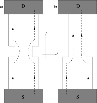
Figure 2.2: The two types of constriction we want to consider. On the left the constriction is localized in a finite region while on the right it is semi-infinite.

We start by considering the case of a finite size constriction. We assume that the system is symmetric with respect to the $x=0$ point and that the length of the constriction is $d$. To keep the analysis simple, we assume that the interaction potentials $V_{1}$ and $V_{2}$ are short ranged on the scale of the density fluctuations: this in particular implies that only points at the same value of the variable $x$ interact and $V_{\alpha,\beta}$ has the form

$$V_{\alpha,\beta}=\left(\begin{array}[]{cc}V_{1}&V_{2}(x)\\ V_{2}(x)&V_{1}\end{array}\right)$$ (2.72)

where

$$V_{2}(x)=\left\{\begin{array}[]{cc}V_{2,1}&x<-d/2\\ V_{2,2}&|x|<d/2\\ V_{2,3}&x>d/2\end{array}\right..$$ (2.73)

The region labelled $1$, $2$ and $3$ are implicitely defined in the piece-wise form of the potential $V_{2}$. We seek for a piece-wise solution. As is standard in scattering theory we label the full solution with the quantum numbers of the incident wave. An “up-moving” solution will then have the form

$$\tilde{\varphi}_{k_{1}}^{u}=\left\{\begin{array}[]{lc}\varphi_{k_{1}}^{u}(x)+r^{u}\varphi^{d}_{k_{1}}(x)&x<-d/2\\ A^{u}\varphi_{k_{2}}^{u}(x)+B^{u}\varphi^{d}_{k_{2}}(x)&|x|<d/2\\ t^{u}\varphi_{k_{3}}^{u}(x)&x>d/2\end{array}\right..$$ (2.74)

The wave vectors in the regions $2$ and $3$ are determined in terms of the incident momentum $k_{1}$ by the conservation of the energy

$$c_{1}k_{1}=c_{2}k_{2}=c_{3}k_{3}$$ (2.75)

where $c_{1}$, $c_{2}$ and $c_{3}$ are the sound velocities in the three regions. In a similar way one can construct the solution for the “down-moving” solution

$$\tilde{\varphi}_{k_{3}}^{d}=\left\{\begin{array}[]{lc}t^{d}\varphi_{k_{3}}^{d}(x)&x<-d/2\\ A^{d}\varphi_{k_{2}}^{d}(x)+B^{d}\varphi^{u}_{k_{2}}(x)&|x|<d/2\\ \varphi_{k_{3}}^{d}(x)+r^{d}\varphi_{k_{3}}^{u}(x)&x>d/2\end{array}\right..$$ (2.76)

In these expressions the spinorial functions $\varphi^{u}_{k}(x)$ and $\varphi^{d}_{k}(x)$ are given by the Eqs. (2.49) and (2.50) where the index $\alpha$ has been dropped for the sake of notation’s simplicity.

The matching conditions are dictated by the physical requirement that there is not energy accumulation at the interfaces. This is equivalent to the requirement of the continuity of the solution at the points $x=\pm d/2$ and gives four conditions to determine the coefficients $A$, $B$, $t$, and $r$ for the up- and down-moving wave functions.

The solution of the set of the equations obtained by imposing the matching conditions can be obtained in a straightforward way. We get, after having expressed the results in terms of the mixing angles,

$$\begin{split}t^{u}&=\frac{e^{-i\frac{k_{1}+k_{3}}{2}d}}{\cos(k_{2}d)\cosh(\theta_{1}-\theta_{3})-i\sin(k_{2}d)\cosh(2\theta_{2}-\theta_{1}-\theta_{3})}\sqrt{\frac{c_{1}}{c_{3}}},\\ r^{u}&=-\frac{\cos(k_{2}d)\sinh(\theta_{1}-\theta_{3})+i\sin(k_{2}d)\sinh(2\theta_{2}-\theta_{1}-\theta_{3})}{\cos(k_{2}d)\cosh(\theta_{1}-\theta_{3})-i\sin(k_{2}d)\cosh(2\theta_{2}-\theta_{1}-\theta_{3})}e^{-ik_{1}d},\\ A^{u}&=\frac{\cosh(\theta_{3}-\theta_{2})e^{-i\frac{k_{1}+k_{2}}{2}d}}{\cos(k_{2}d)\cosh(\theta_{1}-\theta_{3})-i\sin(k_{2}d)\cosh(2\theta_{2}-\theta_{1}-\theta_{3})}\sqrt{\frac{c_{1}}{c_{2}}},\\ B^{u}&=\frac{\sinh(\theta_{3}-\theta_{2})e^{i\frac{k_{2}-k_{1}}{2}d}}{\cos(k_{2}d)\cosh(\theta_{1}-\theta_{3})-i\sin(k_{2}d)\cosh(2\theta_{2}-\theta_{1}-\theta_{3})}\sqrt{\frac{c_{1}}{c_{2}}}.\end{split}$$ (2.77)

The coefficients for the down-moving solution can be obtained by the substitutions

$$t^{u}\to t^{d};~{}r^{u}\to r^{d};~{}A^{u}\to B^{d};~{}B^{u}\to A^{d},$$ (2.78)

and

$$\theta_{1}\to\theta_{3};~{}\theta_{3}\to\theta_{1};~{}c_{1}\to c_{3}.$$ (2.79)

It is easy to verify that the wave function (2.49) with the coefficients determined by (2.77) satisfies the conservation law (2.54).

We recover the case of a semi-infinite constriction by considering the limit $d\to 0$ in the expressions for the transmission and reflection coefficients [35],

$$\begin{split}t^{u}&=\frac{1}{\cosh(\theta_{1}-\theta_{3})}\sqrt{\frac{c_{1}}{c_{2}}},\\ r^{u}&=-\frac{\sinh(\theta_{1}-\theta_{3})}{\cosh(\theta_{1}-\theta_{3})}.\end{split}$$ (2.80)

If one defines the interaction renormalized filling factor $\nu_{i}=\nu e^{-2\theta_{i}}$ for the various region then it is possible to rewrite the above results as

$$\begin{split}r^{u}=&\frac{\nu_{1}-\nu_{3}}{\nu_{1}+\nu_{3}},\\ t^{u}=&\frac{2\nu_{3}}{\nu_{1}+\nu_{3}}\sqrt{\frac{c_{1}}{c_{3}}}.\end{split}$$ (2.81)

These expressions remain valid when we consider the case of two regions with different filling factors [36]. In the following we will consider the symmetric case $\theta_{1}=\theta_{3}$ i.e. the interaction is symmetric with respect to the center of the constriction. From the expressions (2.77) we get

$$\begin{split}t^{u}&=\frac{e^{-ikd}}{\cos(k_{2}d)-i\sin(k_{2}d)\cosh(2\theta_{2}-2\theta_{1})},\\ r^{u}&=-\frac{i\sin(k_{2}d)\sinh(2\theta_{2}-2\theta_{1})}{\cos(k_{2}d)-i\sin(k_{2}d)\cosh(2\theta_{2}-2\theta_{1})}e^{-ikd},\\ A^{u}&=\frac{\cosh(\theta_{1}-\theta_{2})e^{-i\frac{k_{1}+k_{2}}{2}d}}{\cos(k_{2}d)-i\sin(k_{2}d)\cosh(2\theta_{2}-2\theta_{1})}\sqrt{\frac{c_{1}}{c_{2}}},\\ B^{u}&=\frac{\sinh(\theta_{1}-\theta_{2})e^{i\frac{k_{2}-k_{1}}{2}d}}{\cos(k_{2}d)-i\sin(k_{2}d)\cosh(2\theta_{2}-2\theta_{1})}\sqrt{\frac{c_{1}}{c_{2}}}.\end{split}$$ (2.82)

We will use these expressions to calculate the Hall conductance in the presence of a constriction.

The generalizations to the case when many constrictions are present or a constriction connects regions with different filling factors are straightforward.

2.5 The tunneling Hamiltonian

We want now to consider the effect of the tunneling between different edges. The physical origin of tunneling lies in the fact that the electron quasi-particles are not completely localized in one or the other edge i.e. the density matrix $\rho({\bf r},{\bf r^{\prime}})$ has a finite value even if ${\bf r}\not={\bf r^{\prime}}$.

The physics of the tunneling is obviously lost in the hydrodynamical approximation. We need then to insert the tunneling by hand in our Hamiltonian. To do that we need to define a quasi-particle creation operator which adds a quasi-particle with charge $e^{*}$ (not necessarily equal to the electron charge $e$) at the point $x$ of the edge $\alpha$. This is accomplished by requiring that this operator $\Psi^{\dagger}_{\alpha}(x)$ satisfies the commutation relation with the quasi-particle density

$$[\Psi^{\dagger}_{\alpha}(x),\delta\rho_{\beta}(x^{\prime})]=-\frac{e^{*}}{e}\delta_{\alpha,\beta}\delta(x-x^{\prime})\Psi^{\dagger}_{\alpha}(x).$$ (2.83)

At the best of our knowledge there is not exist a general theory which predict the correct value of $e^{*}$ for arbitrary value of the filling factor. For certain values of the filling factor, as an example those given by $\nu=1/(2m+1)$ where $m$ is an integer, it is believed that $e^{*}=\nu e$. Two approaches are then possible. One can fix $e^{*}=\nu e$ and then makes a comparison with the experimental results. On the other hand it is possible to treat $e^{*}$ as a phenomenological parameter determined by the confrontation with the experiment.

The equation (2.83) allows us to express the quasi-particle creation operator in terms of the boson operator via

$$\begin{split}\Psi^{\dagger}_{\alpha}(x)=U^{\dagger}_{\alpha}\exp\left[-i\frac{e^{*}}{e}\sqrt{\frac{2\pi}{\nu}}\sigma_{\alpha,\beta}^{z}\sum_{n>0}\varphi_{n,\beta}^{*}(x)b^{\dagger}_{n}\right]\\ \times\exp\left[-i\frac{e^{*}}{e}\sqrt{\frac{2\pi}{\nu}}\sigma_{\alpha,\beta}^{z}\sum_{n>0}\varphi_{n,\beta}(x)b_{n}\right]\end{split}$$ (2.84)

where the unitary fermion operator $U^{\dagger}_{\alpha}$ commutes with all the boson operators and increases the total charge $Q_{\alpha}$ by $-e^{*}$

$$[U_{\alpha}^{\dagger},Q_{\beta}]=e^{*}\delta_{\alpha,\beta}U^{\dagger}_{\alpha}$$ (2.85)

where the total charge operator is defined as

$$Q_{\alpha}=\int\limits_{-\infty}^{\infty}dx~{}\delta\rho_{\alpha}(x).$$ (2.86)

The solution of the equation (2.83) can be obtained by the observation that the commutation relation can be converted to a differential equation by using the different representations

$$\begin{split}&b\to\frac{\partial}{\partial b^{\dagger}},\\ &b^{\dagger}\to-\frac{\partial}{\partial b},\end{split}$$ (2.87)

which in turn imply that

$$\begin{split}[b,f(b^{\dagger})]=&\frac{\partial f(b^{\dagger})}{\partial b^{\dagger}},\\ [b^{\dagger},g(b)]=&-\frac{\partial g(b)}{\partial b}.\end{split}$$ (2.88)

The operator $U_{\alpha}$ is then the “arbitrary constant” in the solution of the differential equation and its properties can be deduced from the physical insight that it must increases the total charge $Q_{\alpha}$. We have also written the quasi-particle creation operator in a normal ordered way: this will avoid some complications with the normalization [37].

In terms of the quasi-particle operators, the tunneling between the edges coupled by a constriction at $x=0$ is described by the Hamiltonian

$$H_{T}=\Gamma:\Psi_{L}^{\dagger}(0)\Psi_{R}(0):+\Gamma^{*}:\Psi_{R}^{\dagger}(0)\Psi_{L}(0):$$ (2.89)

where $\Gamma$ is the (phenomenological) tunneling amplitude and the symbol $:\ldots:$ indicates the normal ordering. The complete Hamiltonian then reads

$$H=H_{0}+H_{T}=\sum_{n>0}\hbar\omega_{n}b^{\dagger}_{n}b_{n}+\Gamma:\Psi_{L}^{\dagger}(0)\Psi_{R}(0):+\Gamma^{*}:\Psi_{R}^{\dagger}(0)\Psi_{L}(0):$$ (2.90)

where now the tunneling Hamiltonian can be viewed as an interaction Hamiltonian for the bosons and now the total charge in a given edge is not a constant of motion: its time derivative defines a tunnel current operator $I_{T}$ as follows

$$\begin{split}I_{T}&=\frac{i}{\hbar}[H_{T},Q_{L}]\\ &=i\frac{e^{*}}{\hbar}(\Gamma:\Psi_{L}^{\dagger}(0)\Psi_{R}(0):-\Gamma^{*}:\Psi_{R}^{\dagger}(0)\Psi_{L}(0):).\end{split}$$ (2.91)

In the following chapter, when we will deal with the formulation of the transport and derive the relations between the current and voltage, we will describe a method to calculate this tunneling current by defining an exact boson propagator and developing a perturbative scheme to evaluate its expectation value.

We must point out also that we do not specify any statistics for the quasi-particle operator. Wen was able to show that the quasi-particle operator follows a Fermi algebra if and only if $\nu$ is the inverse of an odd integer. If $\nu$ is the inverse of an even integer the quasi-particle follows a Bose algebra. In the intermediate case the quasi-particle has not a definite statistics. We do not restrict the range of variation of the filling fraction and then we do not have real fermion operator for the quasi-particle. We will show in the following that the restriction to fermion operator is not necessary and we can fully develop a perturbative approach to the tunneling.

2.6 The multi-probe setup

In the previous sections of this chapter we have introduced our model for the quantum Hall bar and the way to describe the edges and their excitations. For the sake of simplicity in introducing the notation and the various concepts we have treated the case of two parallel edges with only two probes, namely the drain and the source. However as can be seen from the scheme of the experimental setup in Fig. 1.3 we need to consider a more complicated situation where many probes, edges and contacts are present. To do that we consider the schematic in the Fig. 2.3 where we have introduced six different probes, two of them are used to inject a steady-state current in the system (the D and S probes in the figure) and the others are used to measure either the Hall or the longitudinal voltage. The presence of the constriction is also included.

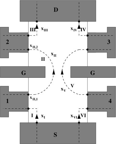
Figure 2.3: A schematization of the experimental device where many edges and probes are represented. The gates (G) create a depletion zone forbidden for the electrons and then force the edges to stay close.

We choose the following notation. Every edge is identified by an arabic figure, while the probes are indicated by roman figures. The point where an edge exits the device is determined by the notation $x_{\alpha,m}$ where $\alpha$ is the arabic figure which refers to the edge, while $m$ identifies the probe. Generally a point belonging to a given edge is identified by its position $x_{\alpha}$ with respect to the edge. The number $x_{\alpha}$ varies in $[-\infty,\infty]$ but we consider that when the electron leaves the device the correlation vanishes exponentially with the increase of the position.

We need to change also the definition of the density and quasi-particle operators. The density fluctuation that belongs to the edge $\alpha$ is now indicated by $\delta\rho(x_{\alpha})$ while the quasi-particle creation operator is $\Psi^{\dagger}(x_{\alpha})$. The simplest way to think at this change of notation is to attach the index $\alpha$ directly to the variable $x$ rather than to the operator. The usefulness of such notation will be proved when we will deal, in the next chapter, with the calculation of the transport properties. When we consider the delta function of the position, namely the quantity $\delta(x_{\alpha}-x_{\beta})$, we identify it with the product of a delta function relative to the edge index times the delta function of the position

$$\delta(x_{\alpha}-x_{\beta})\equiv\delta_{\alpha,\beta}\delta(x-x^{\prime}).$$ (2.92)

The intra-edge interaction is substantially not affected by this change of notation. For the inter-edge interaction we consider that our device is specular with respect to the $x$ axis. In such a way when we consider the interaction potential $V_{2}(x_{\alpha}-x^{\prime}_{\beta})$ we consider two point with the same abscissa belonging to two different edges.

Chapter 3 The formulation of the transport

In this chapter we derive the expression for the conductance matrix in terms of the correlation function of the quasi-particles. In the transport theory we need to calculate the current induced into the reservoir $i$ due to a change in the potential $V_{j}$ of the reservoir $j$. If we consider only the linear relation between the change in the potential $\delta V_{j}$ and the induced current $\delta I_{i}$ we have

$$\delta I_{i}=\sum_{j}G_{ij}({\bf V})\delta V_{j}.$$ (3.1)

As it is recalled in this definition, the conductance matrix $G_{ij}$ is a function of the potential of all the reservoirs. In the following, to simplify the notation, this dependence will be understood even if not indicated explicitely. We choose the convention that a current is defined positive when it enters a reservoir (leaving the system) and negative viceversa. The matrix element $G_{ij}$ are also subjected to the physical conditions

$$\sum_{i}G_{ij}=\sum_{j}G_{ij}=0$$ (3.2)

which represent the gauge invariance and the charge conservation, respectively. These expressions determine the value of the diagonal elements $G_{ii}$ once the off-diagonal elements are known. Notice also that in general there is not other way to calculate these diagonal elements. The rest of the thesis will deal with the calculation of the conductance matrix in various cases study.

3.1 The conductance matrix

We want now to express the conductance matrix in terms of the boson correlation function.

The starting point is the definition of the current of the edge $\alpha$ in terms of the displacement field $\phi$. As we have discussed in the previous chapter this relation can be derived from the continuity equation which gives

$$I(x_{\alpha})=e\partial_{t}\phi(x_{\alpha}).$$ (3.3)

The current in the terminal $i$ is then the algebraic summation of all the currents that enter or leave this terminal. We define the function

$$\xi_{\alpha,i}=\left\{\begin{array}[]{cc}+1&\mbox{if~{}}\alpha\mbox{~{}enters~{}}i\\ -1&\mbox{if~{}}\alpha\mbox{~{}leaves~{}}i\\ 0&\mbox{otherwise}\end{array}\right.$$ (3.4)

such that the current on the terminal $i$ is given by

$$I_{i}=\sum_{\alpha}\xi_{\alpha,i}I(x_{\alpha,i}).$$ (3.5)

This relation and the function $\xi$ represent the mathematical formulation of our convention on the sign of the currents flowing in the system. In general this is the sum of the two different currents, one leaving the terminal and the other entering it. We choose, as the versus of the total current, the versus from the source to the drain in the two edges. This choice fixes the “contact function” $\xi_{\alpha,i}$ and, as we will see, the sign of the potential drops at the contacts.

By remembering that in the linear response theory the voltage is coupled to the charge density, we have

$$\delta I(x_{\alpha},\omega)=i\frac{e^{2}}{\hbar}\sum_{\beta}\int\limits_{-\infty}^{\infty}dx^{\prime}_{\beta}\delta V(x^{\prime}_{\beta})\int\limits_{0}^{\infty}dt\langle[\partial_{t}\phi(x_{\alpha},t),\partial_{{x_{\beta}}^{\prime}}\phi({x_{\beta}}^{\prime})]\rangle e^{i(\omega+i\eta)t}$$ (3.6)

where $\omega$ is the frequency of the external potential and $\langle\ldots\rangle$ is the equilibrium average. We are interested in the static limit hence in the following expressions the limit $\omega\to 0$, when not explicitely indicated, is understood.

After an integration by parts with respect to the time, we arrive at

$$\delta I(x_{\alpha})=i\frac{e^{2}}{h}\sum_{\beta}\int dx^{\prime}_{\beta}~{}[\omega\partial_{x^{\prime}_{\beta}}D(x_{\alpha},x^{\prime}_{\beta};\omega)]\delta V(x^{\prime}_{\beta}),$$ (3.7)

where

$$D(x_{\alpha},x^{\prime}_{\beta};\omega)\equiv-2\pi i\int\limits_{0}^{\infty}\langle[\hat{\phi}(x_{\alpha},t),\hat{\phi}(x^{\prime}_{\beta})]\rangle e^{i(\omega+i\eta)t}dt$$ (3.8)

is the retarded displacement-field propagator, whose explicit expression in terms of “phonon eigenfunctions” is

$$D(x_{\alpha},x^{\prime}_{\beta};\omega)=\nu\sum_{n>0}\left[\frac{\varphi_{n}(x_{\alpha})\varphi_{n}^{*}(x^{\prime}_{\beta})}{\omega-\omega_{n}+i\eta}-\frac{\varphi_{n}^{*}(x_{\alpha})\varphi_{n}(x^{\prime}_{\beta})}{\omega+\omega_{n}+i\eta}\right].$$ (3.9)

In performing the integration by parts we have used the fact that

$$\partial_{{x_{\beta}}^{\prime}}D(x_{\alpha},{x_{\beta}}^{\prime};t=0^{+})=-2\pi[\phi(x_{\alpha}),\partial_{{x_{\beta}}^{\prime}}\phi({x_{\beta}}^{\prime})]\propto\delta(x_{\alpha}-{x_{\beta}}^{\prime})$$ (3.10)

vanishes unless $x_{\alpha}={x_{\beta}}^{\prime}$. We will show in the following that the evaluation of this function on the point $x_{\alpha,i}$ is related to the conductance. However, as we have discussed briefly before, the conductance matrix elements we can calculate are the off-diagonal ones only. Hence in doing these calculations we deal only with the case $x_{\alpha}\not={x_{\beta}}^{\prime}$ and this validates our procedure of integrating by parts.

We need now a model for the external potentials which are applied to the reservoirs. We model only the potentials in the region outside the device. To do that we consider that the potential is uniform in the portion of the edge that runs inside the reservoirs, drops to zero at the contact points between the leads and the device, and is zero inside the device. Thus we choose an external potential which satisfies

$$\partial_{x_{\alpha}}\delta V(x_{\alpha})=\sum_{j}\xi_{\alpha,j}\delta(x_{\alpha}-x_{\alpha,j})\delta V_{j}$$ (3.11)

where the “contact function” was defined in the Eq. (3.4). This expression for the external potential makes very easy to calculate the conductance matrix. Indeed after an integration by parts in the Eq. (3.7), carried out on the assumption that the correlation function decay exponentially for $x\to\pm\infty$, we obtain the expression of the current arriving at the reservoir $i$ via the edge channel $\alpha$ due to a potential variation applied to the edge channel $\beta$ by the reservoir $j$ ($i\not=j$)

$$\begin{split}\delta I_{i}&=\sum_{j}G_{ij}\delta V_{j}\\ &=\sum_{j}\left(-\frac{ie^{2}}{\hbar}\sum_{\alpha,\beta}\xi_{\alpha,i}\xi_{\beta,j}\lim_{\omega\to 0}\omega D(x_{\alpha,i},x_{\beta,j},\omega)\right)\delta V_{j}.\end{split}$$ (3.12)

We have thus obtained an expression for the conductance matrix in terms of the boson correlation function.

As an application we want to calculate this function in the case of two translationally invariant edges. In this case the relation between the energy and the momentum is $\omega=kc$ where $c$ is the phonon velocity and the wave functions are given by the expressions (2.49) and (2.50). To ensure that the wave function vanishes in the limit $|x|\to\infty$ we shift, in the argument of the complex exponential, $k\to k+i\eta\mathrm{sign}(x)$ in the (2.49) and $k\to k-i\eta\mathrm{sign}(x)$ in the (2.50). After plugging in these wavefunctions in the expression for the correlation function we reduce the sum over $k>0$ to the integral over the real axis in $k$. We readily see that only the poles $ck=\pm(\omega+i\eta)$ contribute to the integral thus giving

$$\begin{split}-i\lim_{\omega\to 0}\omega D(x_{\alpha},{x_{\beta}}^{\prime},t)=&\nu\Theta(x_{\alpha}-x^{\prime}_{\beta})\left(\begin{array}[]{cc}u^{2}&-uv\\ -uv&v^{2}\end{array}\right)\\ &+\nu\Theta(x^{\prime}_{\beta}-x_{\alpha})\left(\begin{array}[]{cc}v^{2}&-uv\\ -uv&u^{2}\end{array}\right)\end{split}$$ (3.13)

where the functions $u$ and $v$ are the limits $k\to 0$ of the functions $u_{k}$ and $v_{k}$ we have defined in the (2.51). In the case of non-interacting edges we have $u=1$ and $v=0$, thus we have upward propagation on the left edge and downward propagation on the right edge. This makes the conductance $G_{ij}$ vanishes unless the reservoir $j$ is not “upstream” the reservoir $i$ according to the definition of an ideal Quantum Hall system.

When the edges are interacting, from the direct application of the Eqs. (3.12) and (3.13), we obtain

$$G_{21}=G_{12}=\nu\frac{e^{2}}{h}e^{-2\theta}.$$ (3.14)

Notice that in this simple case an edge contacts both the reservoirs. One might wonder how this result modifies the relation between the current and the source and drain potentials. As pointed out by Wen [14], when the interaction is present, the edge potentials are a linear combination of the source and drain potentials with the coefficients determined by the mixing angle $\theta$. By taking into account this relation we arrive at

$$I=\nu\frac{e^{2}}{h}(V_{S}-V_{D})$$ (3.15)

and this implies that a measure of the Quantum Hall conductance is insensitive to the presence of a translationally invariant inter-edge interaction.

A similar calculation can be developed for the case of a constriction by using the reflection and transmission coefficients in Eq. (2.77). In this case the calculation is complicated by the piece-wise form of the wave functions. To keep the analysis as simple as possible we consider the case when four reservoirs are attached just above and below the constriction and the interaction is present only inside the constriction region (i.e. we fix $\theta_{1}=\theta_{3}=0$). By moving from the wave functions (2.49) and (2.50) we have obtained fixing, as an example, the first reservoir

$$\begin{split}&G_{21}=\nu\frac{e^{2}}{h}\frac{1}{2\pi i}\int\limits_{-\infty}^{\infty}dk\frac{e^{ik(x_{1}-x_{2})}}{k-\omega/c-i0^{+}}t_{k}^{u},\\ &G_{31}=0,\\ &G_{41}=\nu\frac{e^{2}}{h}\frac{1}{2\pi i}\int\limits_{-\infty}^{\infty}dk\frac{e^{-ik(x_{1}+x_{4})}}{k-\omega/c-i0^{+}}r_{k}^{u}.\end{split}$$ (3.16)

With $\theta_{1}=\theta_{3}=0$ the reflection and transmission coefficients read

$$\begin{split}t_{k}^{u}&=\frac{e^{-ik_{1}d}}{\cos(k_{2}d)-i\sin(k_{2}d)\cosh(2\theta_{2})},\\ r_{k}^{u}&=-\frac{i\sin(k_{2}d)\sinh(2\theta_{2})}{\cos(k_{2}d)-i\sin(k_{2}d)\cosh(2\theta_{2})}e^{-ik_{1}d},\end{split}$$ (3.17)

where we have $c_{1}k_{1}=c_{2}k_{2}$. In performing the integration to calculate the conductances we observe that we must close both the integrals in the upper half complex plane. Since $t_{k}$ and $r_{k}$ have only poles inside the integration path in the lower half complex plane, the only pole is at $k=\omega/c+i\eta$ and we obtain

$$\begin{split}&G_{21}=\nu\frac{e^{2}}{h}t^{u}(\omega/c),\\ &G_{41}=\nu\frac{e^{2}}{h}r^{u}(\omega/c).\end{split}$$ (3.18)

The ideal Quantum Hall conductance is recovered by observing that in the limit of vanishing frequency $\omega\to 0$ we have $t^{u}\to 1$ and $r^{u}\to 0$. We are then arrived to the conclusion that the constriction and the interaction do not modify the ideal Quantum Hall conductance. Indeed one must observe that the interaction does not allow for the passage of one quasi-particle from one edge to the other. On the other hand the constriction, in the limit of small energy, becomes fully transparent thus recovering the translationally invariant results.

3.2 The tunneling conductance

When we consider the tunneling, we know that the full Hamiltonian cannot be diagonalizable. Thus we develop a perturbative scheme to calculate the tunneling conductance i.e. the correction to the ideal Quantum Hall conductance induced by the presence of the tunneling. We choose to develop this theory starting from the equations of motion. Such an approach does not rest on any assumptions about the statistics of the quasi-particles and, then, can be applied to the case when $\nu$ is not the inverse of an odd number.

As we have pointed out the presence of the tunneling adds to the free Hamiltonian an interaction potential between the bosons operators. The task at hand is then to calculate the corrections, due to this interaction, to the displacement field $\phi$. We show that this correction can be exactly expressed in terms of a tunneling current propagator and we provide a perturbative evaluation of the latter.

We introduce now some compact notation. We define the phonon spinorial operator

$$B_{n}^{i}\equiv\left(\begin{array}[]{c}b_{n}\\ b_{n}^{\dagger}\end{array}\right)$$ (3.19)

where the index $i\in\{1,2\}$ (the upper part corresponds to $1$), and the associated phonon propagator

$$D_{n,n^{\prime}}^{i,j}(t)\equiv-\frac{i}{\hbar}\Theta(t)\langle[B^{i}_{n}(t),B_{n^{\prime}}^{j\dagger}]\rangle.$$ (3.20)

We define also the spinorial eigenfunction

$$\varphi^{i}_{n}(x_{\alpha})\equiv\left(\begin{array}[]{c}\varphi_{n}(x_{\alpha})\\ \varphi_{n}(x_{\alpha})^{*}\end{array}\right).$$ (3.21)

With these definitions the phonon field propagator can be written as

$$\begin{split}D(x_{\alpha},{x_{\beta}}^{\prime},t)&=\hbar\nu\sum_{i,j}\sum_{\{n,n^{\prime}\}>0}\varphi^{i}_{n}(x_{\alpha})D^{i,j}_{n,n^{\prime}}(t)\varphi^{j}_{n^{\prime}}({x_{\beta}}^{\prime}).\end{split}$$ (3.22)

In the following we will suppress the summation symbols and the sums over repeated indices will be understood. The phonon operator satisfies the equation of motion

$$i\partial_{t}B_{n}^{i}=\Omega_{n}^{i,j}B_{n}^{j}-\frac{Y^{i}_{n}}{e}I_{T}$$ (3.23)

where we have defined

$$\Omega_{n}^{i,j}=\left(\begin{array}[]{cc}\omega_{n}&0\\ 0&-\omega_{n}\end{array}\right),~{}~{}Y^{i}_{n}=\left(\begin{array}[]{c}\gamma_{n}\\ -\gamma^{*}_{n}\end{array}\right),$$ (3.24)

and

$$\gamma_{n}=\sqrt{\frac{2\pi}{\nu}}\sum_{\alpha}\varphi^{*}_{n}(0_{\alpha}).$$ (3.25)

It is now straightforward to verify that the phonon propagator satisfies the equation of motion

$$(i\partial_{t}\delta_{i,l}-\Omega^{i,l}_{n})D^{l,j}_{n,n^{\prime}}=\frac{(-1)^{i}}{\hbar}\delta_{i,j}\delta_{n,n^{\prime}}\delta(t)-\frac{Y^{i}_{n}}{e}{\cal G}^{j}_{n^{\prime}}(t)$$ (3.26)

where the auxiliary operator

$${\cal G}^{i}_{n}(t)=-\frac{i}{\hbar}\Theta(t)\left\langle\left[I_{T}(t),B_{n}^{j\dagger}\right]\right\rangle$$ (3.27)

in turn satisfies

$$(i\partial_{t}\delta_{i,j}-\Omega^{i,j}_{n}){\cal G}^{j}_{n}=-\frac{Y^{i*}_{n}}{e}\tilde{M}_{T}(t)$$ (3.28)

with

$$\tilde{M}_{T}(t)=M_{T}(t)-\frac{{e^{*}}^{2}}{\hbar^{2}}\langle H_{T}\rangle\delta(t)$$ (3.29)

where

$$M_{T}(t)=-\frac{i}{\hbar}\Theta(t)\left\langle\left[I_{T}(t),I_{T}\right]\right\rangle$$ (3.30)

is the tunneling current propagator. We will show later that this propagator can be expressed in terms of the quasi-particle correlation functions.

The Eqs. (3.26) and (3.28) can be readily solved by Fourier transformation to obtain

$$\begin{split}D_{n.n^{\prime}}^{i,j}=&[D^{(0)}]^{i,j}_{n,n^{\prime}}(\omega)\\ &+\frac{\hbar^{2}}{e^{2}}[D^{(0)}]^{i,l}_{n,{n_{1}}}(\omega)Y_{n_{1}}^{l}\tilde{M}_{T}(\omega)(Y_{n_{2}}^{m})^{*}\left([D^{(0)}]^{m,j}_{{n_{2}},n^{\prime}}(\omega)\right)^{*}\end{split}$$ (3.31)

where $[D^{(0)}]^{i,j}_{n,n^{\prime}}(\omega)$ is the noninteracting phonon propagator. Because $\tilde{M}_{T}$ is related to the quasi-particle correlation functions, we have then expressed the phonon propagator in terms of the tunneling current propagator. The noninteracting phonon propagator is determined by the Fourier transformation of the operator

$$[D^{(0)}]^{i,j}_{n,n^{\prime}}(t)=\frac{(-1)^{i}}{\hbar}\delta_{i,j}\delta_{n,n^{\prime}}\delta(t)(i\partial_{t}\delta_{i,j}-\Omega_{n}^{i,j})^{-1}.$$ (3.32)

Notice that there are no approximations on the calculation of the tunneling amplitude. Thus this set of equations constitutes an exact approach to the problem of the tunneling.

Let us denote by $G^{(0)}_{ij}$ the conductance obtained in the absence of tunneling and by

$$\delta G_{ij}=G_{ij}-G^{(0)}_{ij}$$ (3.33)

the correction due to the tunneling. By starting from the definition (3.12), with some straightforward manipulations, one arrives at

$$\begin{split}\delta G_{ij}=&-\frac{i}{\nu^{2}}\lim_{\omega\to 0}\sum_{\alpha_{i}\gamma}\xi_{\alpha i}[D^{(0)}](x_{\alpha i},0_{\gamma};\omega)\\ &\times[\omega\tilde{M}_{T}(\omega)]\sum_{\delta\beta_{j}}[D^{(0)}]^{*}(0_{\delta},x_{\beta j}^{\prime};\omega)\xi_{\beta j}\end{split}$$ (3.34)

where the indices $\gamma$ and $\delta$ run over the two edges that are coupled by tunneling at $x=0$, and the Green’s function of the noninteracting displacement field, $[D^{(0)}]_{\alpha\beta}(x,x^{\prime};\omega)$, is given by Eq. (3.9).

As a concrete example, let us consider a four-terminal geometry, as may be obtained from Fig. 2.3 by considering only the terminals from $1$ to $4$. Let us assume for simplicity that the mixing angle $\theta$ is independent of $x$. Then from Eq. (3.13) we immediately get

$$\begin{split}\sum_{\gamma}[D^{(0)}](x_{\alpha},0_{\gamma};\omega)=&\sum_{\gamma}[D^{(0)}](0_{\gamma},-x_{\alpha};\omega)\\ =&\frac{i\nu}{\omega}e^{-\theta}\left[\Theta(x)\left(\begin{array}[]{c}u\\ -v\end{array}\right)+\Theta(-x)\left(\begin{array}[]{c}-v\\ ~{}u\end{array}\right)\right]\end{split}$$ (3.35)

where the upper (lower) component refers to the left (right) edge and $u=\cosh\theta$, $v=\sinh\theta$.

Substituting this in Eq. (3.34) we find

$$\delta G_{ij}=\sum_{\alpha_{i}\beta_{j}}\delta G_{\alpha_{i}\beta_{j}}(x_{i},x_{j})\xi_{\alpha i}\xi_{\beta j},$$ (3.36)

where

$$\begin{split}\delta G_{\alpha\beta}(x,x^{\prime})=&-ie^{-2\theta}\lim_{\omega\to 0}\frac{\tilde{M}_{T}(\omega)}{\omega}\left\{\Theta(x)\Theta(-x^{\prime})\left(\begin{array}[]{cc}u^{2}&-uv\\ -uv&v^{2}\end{array}\right)\right.\\ &+\Theta(-x)\Theta(x^{\prime})\left(\begin{array}[]{cc}v^{2}&-uv\\ -uv&u^{2}\end{array}\right)+\Theta(x)\Theta(x^{\prime})\left(\begin{array}[]{cc}-uv&u^{2}\\ v^{2}&-uv\end{array}\right)\\ &+\left.\Theta(-x)\Theta(-x^{\prime})\left(\begin{array}[]{cc}-uv&v^{2}\\ u^{2}&-uv\end{array}\right)\right\}.\end{split}$$ (3.37)

Putting this in Eq. (3.36) and noting that $\xi_{\alpha 1}=\xi_{\beta 4}=1$, $\xi_{\alpha 2}=\xi_{\beta 3}=-1$ (with the labels $i$, $j$ as specified in the figure) we finally obtain the correction to the Landauer-Büttiker conductances of the ideal system:

$$\delta G_{ij}=ie^{-2\theta}\lim_{\omega\to 0}\frac{{\tilde{M}}_{T}(\omega)}{\omega}\left(\begin{array}[]{cccc}uv&v^{2}&-uv&-v^{2}\\ u^{2}&uv&-u^{2}&-uv\\ -uv&-v^{2}&uv&v^{2}\\ -u^{2}&-uv&u^{2}&uv\end{array}\right).$$ (3.38)

In the following for simplicity of notation we define the function

$$g_{T}\equiv i\lim_{\omega\to 0}\frac{M_{T}(\omega)}{\omega}.$$ (3.39)

We consider the specific setup of Fig. 2.3 which represent an ideal representation of the experimental setup proposed by Roddaro et al. [28]. The resistance $R_{xx}$ of the quantum point contact is measured between terminals 3 and 4

$$R_{xx}=\frac{V_{4}-V_{3}}{I},$$ (3.40)

where $I$ is the source-to-drain current. By considering that the constriction does not affect the source and drain probes, the full conductance matrix reads

$$G_{ij}=\frac{e^{2}}{h}\nu\left(\begin{array}[]{cccccc}1&0&0&0&0&-1\\ 0&1&0&-1&0&0\\ -1&0&1+\delta g_{11}&\delta g_{12}&\delta g_{13}&\delta g_{14}\\ 0&0&-1+\delta g_{21}&1+\delta g_{22}&\delta g_{23}&\delta g_{24}\\ 0&-1&\delta g_{31}&\delta g_{32}&1+\delta g_{33}&\delta g_{34}\\ 0&0&\delta g_{41}&\delta g_{42}&-1+\delta g_{43}&1+\delta g_{44}\end{array}\right),$$ (3.41)

where the indices $i$, $j$ run over $\{S,D,1,2,3,4\}$ and the right bottom submatrix is given by $\delta g_{ij}=\frac{h\delta G_{ij}}{\nu e^{2}}$. In the next chapter we will evaluate the $g_{T}$ in a perturbative way where the small parameter is the tunneling amplitude $\Gamma$: we will show that the leading term in $\delta G_{ij}$ is proportional to $|\Gamma|^{2}$ hence it must constitute a small correction to the ideal Quantum Hall conductance. In the Appendix C we discuss briefly the Landauer-Büttiker formalism and give some insights about the calculation of this matrix. As it is customary in the experimental setup we fix $V_{D}=0$, $I_{S}=-I_{D}=-I$ and $I_{1}=I_{2}=I_{3}=I_{4}=0$. With these constraints, the equation (3.1) can be easily solved, and to the lowest non vanishing order in $g_{T}$ we get

$$R_{xx}=\frac{h^{2}}{\nu^{2}e^{4}}e^{-2\theta}(u+v)u~{}g_{T}=\frac{h^{2}}{\nu^{2}e^{4}}e^{-\theta}\cosh{\theta}~{}g_{T}.$$ (3.42)

Notice that this perturbative result is valid only so long as $R_{xx}$ is much smaller that $\frac{h}{e^{2}}$: The tunneling amplitude $\Gamma$ must be sufficiently small to justify this perturbative approach.

3.3 The tunneling amplitude

In the previous section we have connected the conductance matrix to the current-current correlation function $\tilde{M}_{T}$. The next step is to connect this function with the quasi-particle correlation function. In this step we introduce a perturbative approach and develop all the terms to the second order in the tunneling amplitude $\Gamma$.

In $\tilde{M}_{T}$ two terms are present. The first one is the current-current correlation function proportional to $\langle[I_{T}(t),I_{T}]\rangle$. Because the tunneling current $I_{T}$ is proportional to $|\Gamma|$ this correlation function is already second order in the tunneling amplitude. The second term is the average on the ground state of the operator $H_{T}$. This average must be calculated to the second order in $|\Gamma|$. By using the Kubo formula [32] we arrive at

$$\langle H_{T}(t)\rangle=\frac{i}{\hbar}\int\limits_{-\infty}^{t}dt^{\prime}~{}\langle[H_{T}(t^{\prime}),H_{T}(t)]\rangle.$$ (3.43)

To simplify the notation we define the operator

$$A(t)=:\Psi_{L}^{\dagger}(0,t)\Psi_{R}(0,t):$$ (3.44)

and then write the tunneling Hamiltonian as

$$H_{T}(t)=\Gamma A(t)+\Gamma^{*}A^{\dagger}(t)$$ (3.45)

and the tunneling current as

$$I_{T}(t)=\frac{ie^{*}}{\hbar}(\Gamma A(t)-\Gamma^{*}A^{\dagger}(t))$$ (3.46)

where we have used the fact that the tunneling takes place at the point $x=0$. In this notation we have then

$$\langle[H_{T}(t^{\prime}),H_{T}(t)]\rangle=|\Gamma|^{2}(\langle[A(t),A^{\dagger}(t^{\prime})]\rangle+\langle[A^{\dagger}(t),A(t^{\prime})]\rangle)$$ (3.47)

and

$$\langle[I_{T}(t),I_{T}(0)]\rangle=\frac{{e^{*}}^{2}}{\hbar^{2}}|\Gamma|^{2}(\langle[A(t),A^{\dagger}(0)]\rangle+\langle[A^{\dagger}(t),A(0)]\rangle).$$ (3.48)

Notice that in doing these averages the anomalous means that involved two $A$ or two $A^{\dagger}$ operator have been dropped. This is justified by the presence of the operator $U_{\alpha}$ in the definition of the quasi-particle operator. Indeed, being unitary operators, we have $U_{R}^{\dagger}U_{R}=U_{L}^{\dagger}U_{L}\equiv 1$ while the averages of the others product of two $U$ operators is zero. We have restored here the left $L$ and right $R$ notation for the sake of simplicity. Indeed in the constriction only two edges are present (we do not have any contact inside the constriction). Notice also that we have chosen the coordinate systems in these edges to have the $x=0$ point at the same height of the sample.

The simple relation between a commutator and its hermitian conjugate

$$[A,B]^{\dagger}=-[A^{\dagger},B^{\dagger}],$$ (3.49)

if we define the correlation functions

$$\begin{split}&G_{-}(t;t^{\prime})=\langle A(t^{\prime})A^{\dagger}(t)\rangle,\\ &G_{+}(t;t^{\prime})=\langle A^{\dagger}(t)A(t^{\prime})\rangle,\end{split}$$ (3.50)

allows us to recast the average of the tunneling Hamiltonians commutator as

$$\begin{split}\langle[H_{T}(t^{\prime}),H_{T}(t)]\rangle=&|\Gamma|^{2}\left(\langle[A^{\dagger}(t),A(t^{\prime})]\rangle-\langle[A^{\dagger}(t),A(t^{\prime})]\rangle^{\dagger}\right)\\ =&2i|\Gamma|^{2}\mbox{Im}(G_{-}(t^{\prime};t)-G_{+}(t^{\prime};t))\\ =&4i|\Gamma|^{2}\mbox{Im}G_{-}(t^{\prime};t)\end{split}$$ (3.51)

where we have used the relation $G_{+}(t^{\prime};t)=G_{-}^{*}(t^{\prime};t)$ that we will prove in the following chapter. The tunneling current correlation function can be rewritten as

$$\langle[I_{T}(t),I_{T}]\rangle=-4i\frac{{e^{*}}^{2}}{\hbar}|\Gamma|^{2}\mbox{Im}G_{-}(t;0).$$ (3.52)

Because by definition we have

$$\tilde{M}_{T}(\omega)=M_{T}(\omega)-\frac{{e^{*}}^{2}}{\hbar^{2}}\\ \int\limits_{-\infty}^{\infty}dt~{}\delta(t)\langle H_{T}(t)\rangle e^{i\omega t}$$ (3.53)

we must calculate the Fourier transform of the tunneling correlation function and of the second term in the right hand side. To calculate this second term we use the Dirac $\delta$ to perform the integration on time and we have

$$\begin{split}\int\limits_{-\infty}^{\infty}dt~{}\delta(t)\langle H_{T}(t)\rangle e^{i\omega t}&=-4\frac{|\Gamma|^{2}}{\hbar}\int\limits_{-\infty}^{0}dt^{\prime}~{}\mbox{Im}G_{-}(t^{\prime};0)\\ &=-4\frac{|\Gamma|^{2}}{\hbar}\int\limits_{0}^{\infty}dt^{\prime}~{}\mbox{Im}G_{-}(-t^{\prime};0)\\ &=4\frac{|\Gamma|^{2}}{\hbar}\int\limits_{0}^{\infty}dt^{\prime}~{}\mbox{Im}G_{-}(t^{\prime};0)\end{split}$$ (3.54)

where we have used the fact $G_{-}(t;0)=G_{+}^{*}(t;0)=G_{+}(-t;0)$ we will prove in the next chapter. It is now easy to obtain the relation between $\tilde{M}_{T}(\omega)$ and the function $G_{-}(t)$. We get

$$\begin{split}\lim_{\omega\to 0}\frac{\tilde{M}_{T}(\omega)}{\omega}=&-\frac{4{e^{*}}^{2}|\Gamma|^{2}}{\hbar^{3}}\left[\lim_{\omega\to 0}\int\limits_{0}^{\infty}dt~{}\frac{\cos(\omega t)-1}{\omega}\mbox{Im}G_{-}(t)\right.\\ &\left.+i\lim_{\omega\to 0}\int\limits_{0}^{\infty}dt~{}\frac{\sin(\omega t)}{\omega}\mbox{Im}G_{-}(t)\right]\\ =&-\frac{4i{e^{*}}^{2}|\Gamma|^{2}}{\hbar^{3}}\int\limits_{0}^{\infty}dt~{}t\mbox{Im}G_{-}(t).\end{split}$$ (3.55)

The presence of a bias voltage $V_{\alpha}$ on the edge $\alpha$ modifies the time evolution of the corresponding quasi-particle operator

$$\hat{\Psi}^{\dagger}(x_{\alpha},t)\to\hat{\Psi}^{\dagger}(x_{\alpha},t)e^{-i\frac{e^{*}V_{\alpha}t}{\hbar}}.$$ (3.56)

The underlying physical assumption is, of course, that each edge is in equilibrium with a reservoir, from which it generates, at potential $V_{\alpha}$. Under this assumption, the bias voltage dependence of the conductances can be calculated with no additional effort. Indeed the function $G_{-}$ can be easily expressed in terms of the quasi-particle creation and annihilation operators. From the definition we have

$$\begin{split}G_{-}(t;t^{\prime})&=\langle A(t^{\prime})A^{\dagger}(t)\rangle\\ &=\langle:\Psi_{L}^{\dagger}(0,t^{\prime})\Psi_{R}(0,t^{\prime})::\Psi_{R}^{\dagger}(0,t)\Psi_{L}(0,t^{\prime}):\rangle\end{split}$$ (3.57)

thus this correlation function is modified by a phase factor due to the presence of the finite edge voltages. Notice that the same phase factor modifies the function $G_{+}$.

With arguments similar to those used to derive the Eq. (3.55) we have

$$\begin{split}\langle[H_{T}(t^{\prime}),H_{T}(t)]\rangle&=4i\cos(\omega_{T}t^{\prime})\mbox{Im}G_{-}(t^{\prime};t),\\ \langle[I_{T}(t),I_{T}]\rangle&=-\frac{4i{e^{*}}^{2}}{\hbar^{3}}\cos(\omega_{T}t)\mbox{Im}G_{-}(0;t),\end{split}$$ (3.58)

and

$$\begin{split}g_{T}(\omega_{T})\equiv i\lim_{\omega\to 0}\frac{\tilde{M}_{T}(\omega)}{\omega}=&\frac{4{e^{*}}^{2}|\Gamma|^{2}}{\hbar^{3}}\int\limits_{0}^{\infty}dt~{}t\cos(\omega_{T}t)\mbox{Im}G_{-}(t;0)\\ =&\frac{4{e^{*}}^{2}|\Gamma|^{2}}{\hbar^{3}}\frac{\partial}{\partial\omega_{T}}\int\limits_{0}^{\infty}dt~{}\sin(\omega_{T}t)\mbox{Im}G_{-}(t;0)\\ =&\frac{4{e^{*}}^{2}|\Gamma|^{2}}{\hbar^{3}}\frac{\partial}{\partial\omega_{T}}\mbox{Im}\int\limits_{0}^{\infty}dt~{}e^{i\omega_{T}t}\mbox{Im}G_{-}(t;0),\end{split}$$ (3.59)

where we have defined the frequency

$$\omega_{T}=\frac{{e^{*}}V_{T}}{\hbar}.$$ (3.60)

We evaluate the tunneling voltage, the voltage across the quantum point contact, by

$$V_{T}=\frac{V_{1}-V_{2}}{2}+\frac{V_{3}-V_{4}}{2}$$ (3.61)

and it is possible to prove that $V_{T}=V_{H}$ where $V_{H}$ is the Hall voltage. The amplitude $g_{T}(\omega_{T})$ must be plugged in the Eq. (3.38) to calculate the correction to the ideal conductance. The result of this operation is the main topic of the next chapter.

Chapter 4 The transport properties in the presence of the constriction

In this chapter we apply the formalism we have developed in the previous chapter to the case when the tunneling takes place inside the constriction.

We need to calculate the retarded response function $G_{-}(x_{\alpha},{x_{\beta}}^{\prime},t)$ defined as

$$G_{-}(x,t;x^{\prime},t^{\prime})=\left\langle:\Psi_{L}^{\dagger}(x^{\prime},t^{\prime})\Psi_{R}(x^{\prime},t^{\prime})::\Psi_{R}^{\dagger}(x,t)\Psi_{L}(x,t):\right\rangle.$$ (4.1)

To do this calculation we use the Haussdorf lemma

$$e^{A}e^{B}=e^{B}e^{A}e^{[A,B]}$$ (4.2)

and the expression of the operator $\Psi$ in terms of the boson operators as defined in Eq. (2.84).

We start by considering the zero temperature limit and obtain an approximated form of this correlation function. The presence of the constriction introduces the time scale, $t_{0}=d/c$, i.e. the time a density fluctuation needs to travel through the constriction. We can then write the correlation function as the sum of two different contributions, one for $t<t_{0}$ and the other for $t>t_{0}$. This allows us to perform the Fourier transform we need to calculate the current.

The non-zero temperature case is then recovered by a conformal transformation [38] that allows us to obtain the form of the correlation function directly from the zero temperature expression. Also in this case the correlation function can be separated in two different contributions for short and long times.

4.1 General results

By plugging in the definition of the $G_{-}(x,t;x^{\prime},t^{\prime})$ correlation function the general form of the quasi-particle operator $\Psi^{\dagger}(x_{\alpha})$ given by the Eq. (2.84) we get

$$\begin{split}G_{-}(x,t;x^{\prime},t^{\prime})=&\exp\left[\frac{2\pi{e^{*}}^{2}}{\nu e^{2}}\sum_{n>0}\left(\varphi_{nR}(x)+\varphi_{nL}(x)\right)\right.\\ &\left.\times\left(\varphi_{nR}^{*}(x^{\prime})+\varphi_{nL}^{*}(x^{\prime})\right)e^{i\omega_{k}(t-t^{\prime})}\right]\end{split}$$ (4.3)

while when we perform the same calculation on $G_{+}(x,t;x^{\prime},t^{\prime})$ we have

$$\begin{split}G_{+}(x,t;x^{\prime},t^{\prime})=&\exp\left[\frac{2\pi{e^{*}}^{2}}{\nu e^{2}}\sum_{n>0}\left(\varphi_{nR}^{*}(x)+\varphi_{nL}^{*}(x)\right)\right.\\ &\left.\times\left(\varphi_{kR}(x^{\prime})+\varphi_{kL}(x^{\prime})\right)e^{-i\omega_{k}(t-t^{\prime})}\right].\end{split}$$ (4.4)

To obtain these relations we have used the fact that the temperature is zero. In this case the average of the boson operator exponentials on the ground state gives

$$\langle e^{\alpha b^{\dagger}_{n}}e^{\beta b_{n}}\rangle=1$$ (4.5)

where $\alpha$ and $\beta$ are arbitrary coefficients. We will see that in the case of non-zero temperature this average is a function of the temperature via the Bose distribution.

From these expressions we get immediately the relations

$$G_{-}(x,t;x^{\prime},t^{\prime})=G_{+}^{*}(x,t;x^{\prime},t^{\prime})$$ (4.6)

and if we fix $x=x^{\prime}=0$ we have also

$$G_{-}(0,t;0,0)\equiv G_{-}(t)=G_{+}(-t).$$ (4.7)

This validates our results obtained in the previous chapter about the relation between the tunneling amplitude and the $G_{-}(t)$ correlation function. Notice that now and in the following we use the fact that the times $t$ and $t^{\prime}$ appear always in the combination $t-t^{\prime}$ to set $t^{\prime}\equiv 0$. When we fix $x=x^{\prime}=0$ we obtain

$$\begin{split}G_{-}(t)=&\exp\left[\frac{2\pi{e^{*}}^{2}}{\nu e^{2}}\sum_{n>0}\left|\varphi_{nR}(0)+\varphi_{nL}(0)\right|^{2}e^{i\omega_{k}t}\right].\end{split}$$ (4.8)

To calculate the effects of the constriction we substitute in the Eq. (4.3) the wave functions $\varphi$ determined in this case. The result of this operation is

$$\begin{split}G_{-}(x,t;x,&t^{\prime})=\exp\left[\frac{2\pi{e^{*}}^{2}}{L\nu e^{2}}e^{-2\theta_{2}}\sum_{k_{2}>0}\frac{e^{ik_{2}c_{2}(t-t^{\prime})}}{k_{2}}\right.\\ &\left.\phantom{\frac{{e^{*}}^{2}}{L}}\times\left(|A^{u}e^{ik_{2}x}-B^{u}e^{-ik_{2}x}|^{2}+|A^{d}e^{-ik_{2}x}-B^{d}e^{ik_{2}x}|^{2}\right)\right]\end{split}$$ (4.9)

where the coefficients $A^{u}$, $B^{u}$, $A^{d}$ and $B^{d}$ are given by (2.77). By assuming that the tunneling is localized at the point $x=x^{\prime}=0$ and that the system is symmetric with respect to the center of the constriction, i.e. we assume $\theta_{1}=\theta_{3}$, and substituting the expression (2.77) in this equation we obtain our key result

$$\begin{split}G_{-}(t)=&\exp\left[\frac{4\pi{e^{*}}^{2}}{L\nu e^{2}}\frac{\cosh(2\theta_{2})}{\cosh(2\theta_{1})}e^{-2\theta_{2}}\sum_{k_{2}>0}\frac{e^{ik_{2}c_{2}t}}{k_{2}}\right.\\ &\times\left.\left(\frac{\cosh(2\theta_{12})-\sinh(2\theta_{12})\cos(k_{2}d)}{1+2\sinh^{2}(\theta_{12})\sin^{2}(k_{2}d)}\right)\right]\end{split}$$ (4.10)

where we have defined $\theta_{12}=\theta_{1}-\theta_{2}$.

4.2 The translationally invariant system

Let us discuss, starting from the Eq. (4.10) the case of translationally invariant edges. To do that we fix $\theta_{1}=\theta_{2}=\theta$. With this position the correlation function (4.10) greatly simplifies to give

$$G_{-}(t)=\exp\left[\frac{4\pi{e^{*}}^{2}}{L\nu e^{2}}e^{-2\theta}\sum_{k>0}\frac{e^{ikct}}{k}\right].$$ (4.11)

To calculate this expression we use the well known analytical results

$$\begin{split}&\sum_{n=1}^{\infty}\frac{\cos(nq)}{n}=-\frac{1}{2}\ln(2-2\cos(q))\\ &\sum_{n=1}^{\infty}\frac{\sin(nq)}{n}=\frac{1}{2}(\pi-q)\end{split}$$ (4.12)

which can be summarized in

$$\sum_{n=1}^{\infty}\frac{e^{inq}}{n}=-\ln\left(1-e^{iq}\right).$$ (4.13)

If $q$ is small compared to $1$ we have the approximated results

$$\begin{split}\sum_{n=1}^{\infty}\frac{\cos(nq)}{n}\simeq-\ln(q),~{}\sum_{n=1}^{\infty}\frac{\sin(nq)}{n}\simeq\frac{\pi}{2},~{}\sum_{n=1}^{\infty}\frac{e^{inq}}{n}\simeq-\ln(iq).\end{split}$$ (4.14)

To calculate the expression (4.11) we write the momentum $k$ in terms of a integer $j$ defined by $k=2\pi j/L$ and then evaluate the series in $j$ to obtain

$$G_{-}(t)=\exp\left[-\frac{2{e^{*}}^{2}}{\nu e^{2}}e^{-2\theta}\ln\left(1-e^{\frac{2\pi ict}{L}-\delta}\right)\right]$$ (4.15)

and in the limit of large system size $ct/L\ll 1$ we have

$$G_{-}(t)=\left(\delta-\frac{2\pi ict}{L}\right)^{-\frac{2}{\nu}\frac{{e^{*}}^{2}}{e^{2}}e^{-2\theta}}$$ (4.16)

where $\delta$ assures the convergence of the series even when $t\to 0$. This function is the propagator for the Luttinger Liquid model, with the anomalous exponent $\frac{2}{\nu}\frac{{e^{*}}^{2}}{e^{2}}e^{-2\theta}$. Notice that if we assume $e^{*}=\nu e$ we get for this exponent

$$2\nu e^{-2\theta}=2\tilde{\nu}.$$ (4.17)

In this case the tunneling differential conductance at zero temperature is predicted to have a power law behavior with exponent given by $2({e^{*}/e})^{2}/\tilde{\nu}-2$. In fact to obtain the relation between the tunneling current and the tunneling voltage we must evaluate the Eq. (3.59). To perform this calculation we introduce a Heaviside function, $\Theta(t)$, to extend the integral over the real axis and then we evaluate the Fourier transform by calculating the convolution between the Fourier transforms of the $G_{\pm}(t)$ and of the $\Theta(t)$. Some details on the calculation of Fourier transform of the $G_{\pm}(t)$ are discussed in the Appendix D. The result of these operations is the tunneling amplitude

$$\begin{split}g_{T}(\omega_{T})=&\frac{2\pi|\Gamma|^{2}{e^{*}}^{2}}{\hbar^{3}\Gamma(\alpha)}\left(\frac{L}{2\pi c}\right)^{\alpha}\frac{d}{d\omega_{T}}|\omega_{T}|^{\alpha-1}\mathrm{sign}(\omega_{T})\end{split}$$ (4.18)

where we have defined

$$\alpha=\frac{2}{\nu}\frac{{e^{*}}^{2}}{e^{2}}e^{-\theta}.$$ (4.19)

The Eq. (4.18) reproduces the result of Wen for the tunneling at zero temperature in the translationally invariant case [14]. We want to point out that in the calculation of Wen a ultraviolet cut-off determined by the magnetic length scale appears. This cut-off is necessary if one evaluates the sum in the correlation function as an integral to guarantee the convergence. In our case however an infrared cut-off determined by the sample length $L$ appears. The finiteness of this length assures the convergence of the series in the $G_{-}$ correlation function eliminating the singularity at $k\to 0$.

When we consider the finite temperature case we must evaluate the boson thermal average $\langle b^{\dagger}_{n}b_{n}\rangle$ which appears in the argument of the exponential in the definition of the $G_{-}$ correlation function. The result of this evaluation is that the correlation function at finite temperature can be obtained from that at zero temperature by the conformal transformation [38]

$$\left(\delta\pm it\right)\to\frac{\sin[\pi T(\delta\pm it)]}{\pi T}~{}.$$ (4.20)

Notice that we are using units in which $\hbar=k_{B}=1$, where $k_{B}$ is the Boltzmann constant. The correct physical dimensions are restored via the substitution $T\to k_{B}T/\hbar$ and this is understood in the following equations. With this substitution the evaluation of the $g_{T}$ function follows the same steps we have discussed in the zero temperature case. In this case however one must evaluate the integral

$$\int_{-\infty}^{\infty}dt~{}e^{i\omega t}\frac{(\pi Tt)^{\alpha}}{\sinh^{\alpha}(\pi tT)}.$$ (4.21)

The evaluation of this integral is discussed in the Appendix D. We have thus obtained

$$\begin{split}g_{T}(\omega_{T},T)=&2^{\alpha+1}\frac{{e^{*}}^{2}|\Gamma|^{2}}{\hbar^{3}}\left(\frac{L}{2\pi c}\right)^{\alpha}(\pi T)^{\alpha-1}\sin\left(\frac{\pi\alpha}{2}\right)\\ &\times\frac{\partial}{\partial\omega_{T}}\mathrm{Im}B\left(\frac{\alpha}{2}-i\frac{\omega_{T}}{2\pi T},1-\alpha\right)\end{split}$$ (4.22)

where $B$ is the Euler Beta function defined by [21]

$$B(\alpha,\beta)=\frac{\Gamma(\alpha)\Gamma(\beta)}{\Gamma(\alpha+\beta)}.$$ (4.23)

With some straightforward manipulations on the $B$ function we can recover the result of Wen [14] for the finite temperature tunneling conductance.

4.3 The effect of the constriction

We consider now the effect of the constriction which breaks the translational invariance. To do that we must evaluate the sum which compares in the $G_{-}$ correlation function in the Eq. (4.10). We define the quantity

$$\begin{split}S_{-}(t,d)=&\frac{2\pi}{L}\frac{\cosh(2\theta_{2})}{\cosh(2\theta_{1})}\\ &\times\sum_{k_{2}>0}\frac{e^{ik_{2}c_{2}t}}{k_{2}}\left(\frac{\cosh(2\theta_{12})-\sinh(2\theta_{12})\cos(k_{2}d)}{1+2\sinh^{2}(\theta_{12})\sin^{2}(k_{2}d)}\right)\end{split}$$ (4.24)

and in the following we will evaluate it numerically. We then separates its real and imaginary parts

$$\begin{split}ReS_{-}(t,d)=&\sum_{n=1}^{\infty}\frac{\cosh(2\theta_{12})-\sinh(2\theta_{12})\cos(2\pi dn/L_{2})}{1+2\sinh^{2}\theta_{12}\sin^{2}(2\pi dn/L_{2})}\\ &\times\frac{\cos(2\pi nc_{2}t/L_{2})}{n},\\ ImS_{-}(t,d)=&\sum_{n=1}^{\infty}\frac{\cosh(2\theta_{12})-\sinh(2\theta_{12})\cos(2\pi dn/L_{2})}{1+2\sinh^{2}\theta_{12}\sin^{2}(2\pi dn/L_{2})}\\ &\times\frac{\sin(2\pi c_{2}tn/L_{2})}{n}.\end{split}$$ (4.25)

Notice that in these functions we have defined the integer $n$ such that $k_{2}=2\pi n/L_{2}$ and the length $L_{2}$, defined by

$$L_{2}=L\frac{\cosh(\theta_{1})}{\cosh(\theta_{2})},$$ (4.26)

which takes into account the different propagation velocities of the wave function in the regions $1$ and $2$. The convergence of the series is guaranteed by the oscillatory behavior of the trigonometric functions.

The constriction introduces the characteristic time $t_{0}=d/c_{2}$ which is the time an edge wave needs to travel through the constriction. We discuss the two limits of $t\gg t_{0}$ and $t\ll t_{0}$. In both these two limits we recover an expression for the $G_{-}$ correlation function which is similar to the translationally invariant case and this allows us to obtain the tunneling conductance.

First let us consider the $d\to 0$ regime. From the Eq. (4.25) we get

$$\begin{split}ReS_{-}(t,d\to 0)=&e^{-2\theta_{12}}\\ &\times\left[-\frac{1}{2}\ln\left(2-2\cos\left(\frac{2\pi c_{2}t}{L_{2}}\right)\right)\right]\\ \simeq&-e^{-2\theta_{12}}\ln(2\pi c_{2}t/L_{2}),\\ ImS_{-}(t,d\to 0)=&e^{-2\theta_{12}}\left(\frac{\pi}{2}(1-4c_{2}t/L_{2})\right)\\ \simeq&e^{-2\theta_{12}}\frac{\pi}{2}.\end{split}$$ (4.27)

By plugging in these results in the expression for the $G_{-}$ correlation function we get

$$G_{-,d\to 0}(t)=\left(\delta-\frac{2\pi ic_{2}t}{L_{2}}\right)^{-\frac{2}{\nu}\frac{{e^{*}}^{2}}{e^{2}}e^{-2\theta_{1}}}.$$ (4.28)

From the definition (4.26) and from the energy conservation $k_{1}c_{1}=k_{2}c_{2}$ we have also the relation

$$\frac{L_{2}}{c_{2}}=\frac{L}{c_{1}}.$$ (4.29)

With this result we recover the same correlation function of the translationally invariant case when the constriction is not present.

In the other limit $d\to\infty$ we have substituted in the two functions in the Eq. (4.25) the averaged values, $\langle\cos(k_{2}d)\rangle=0$, $\langle\sin^{2}(k_{2}d)\rangle=1/2$ obtaining

$$\begin{split}ReS_{-}(t,d\to\infty)=&(1+\tanh^{2}(\theta_{12}))\\ &\times\left[-\frac{1}{2}\ln\left(2-2\cos\left(\frac{2\pi c_{2}t}{L_{2}}\right)\right)\right]\\ \simeq&-(1+\tanh^{2}(\theta_{12}))\ln(2\pi c_{2}t/L_{2}),\\ ImS_{-}(t,d\to\infty)=&(1+\tanh^{2}(\theta_{12}))\left(\frac{\pi}{2}(1-2c_{2}t/L_{2})\right)\\ \simeq&(1+\tanh^{2}(\theta_{12}))\frac{\pi}{2}.\end{split}$$ (4.30)

Again when we consider the function $G_{-}(t)$ we get a power law of $t$

$$G_{-,d\to\infty}(t)=\left(\delta-\frac{2\pi ic_{2}t}{L_{2}}\right)^{-\frac{2}{\nu}\frac{{e^{*}}^{2}}{e^{2}}e^{-2\theta_{2}}(1+\tanh^{2}(\theta_{12}))}.$$ (4.31)

In this case the presence of the constriction affects the exponent of this correlation function and can change the behavior of the tunneling amplitude.

The two limits of short and long times (with respect to $t_{0}$) are clearly visible in the numerical evaluation of the function $S_{-}(t,d)$ as shown in the Fig. 4.1.

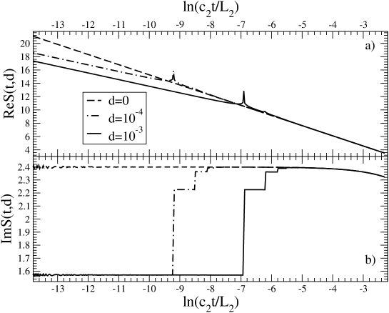
Figure 4.1: a) Plot of $ReS_{-}(t,d)$ vs. $\ln(c_{2}t/L_{2})$ for various values of $d$. Observe the two different regimes for $c_{2}t>d$ and $c_{2}t<d$. The two slopes agree very well with the approximated result of Eq.(4.24). We have chosen $\exp(\theta_{12})=1.5275$ in this calculation. b) Plot of $ImS(t,d)$ vs. $\ln(c_{2}t/L_{2})$ for various values of $d$. We used the same parameters as a). The values for small and large $c_{2}t/L_{2}$ agree well with the expected results (see Eqs.(4.27) and (4.30)). The downward curvature at large times arises from the finite size of the system used in the numerical calculation and disappears in the limit of large system size.

In the numerical calculation we have fixed the value of $d$ and $\theta_{12}$ and then varied the value of $c_{2}t$. As it is seen from the Fig. 4.1 the two limits we have discussed are reached for $c_{2}t\gg d$ and $c_{2}t\ll d$. In the Fig. 4.1 we report the behavior of the functions $ReS$ and $ImS$ vs. the time for some values of $d$ and fixed $\theta_{12}$. Notice that we have restricted our calculation to the case $c_{2}t/L_{2}\ll 1$ and $d/L\ll 1$. The agreement of the calculated expressions and the approximated results (4.27) and (4.30) is very good.

Hence from now on we approximate the $S_{-}(t,d)$ function as the sum of the long and short time behaviors

$$\begin{split}S_{-}(t,d)=&\Theta(t-t_{0})S_{-}(t,d\to 0)\\ &+\Theta(t_{0}-t)(S_{-}(t,d\to\infty)-\Delta_{-})\end{split}$$ (4.32)

where the $\Delta_{-}$ function assures the continuity of $S_{-}$ at the point $t=t_{0}$. The two functions $S_{-}(t,d\to 0)$ and $S_{-}(t,d\to\infty)$ are given by the limits for long and short times of the function $ReS$ and $ImS$, respectively.

With this approximation we have separated the calculation of the tunneling correlation function $G_{-}$ in the calculation of the short and long times behaviors. As we have seen these behaviors are similar to the translationally invariant case. We then expect that the low energy behavior (which corresponds to the low bias voltage region) of the conductance will be dominated by the long time part of $S_{-}(t,d)$. Vice-versa, the response to a high bias voltage will be dominated by the short time behavior of $S_{-}(t,d)$. Within this approximation the $G_{-}(t,d)$ reads

$$\begin{split}G_{-}(t)=\Theta(t-t_{0})G_{-,d\to 0}(t)+\Theta(t_{0}-t)G_{-,d\to\infty}(t)\exp\left[-\frac{2{e^{*}}^{2}}{e^{2}\nu}e^{-2\theta_{2}}\Delta_{-}\right]\end{split}$$ (4.33)

where the exponential factor in the second term in the right hand side stems from the presence of the constant $\Delta_{-}$.

We have thus obtained the expression for the $G_{-}$ correlation function when the constriction is present. The next step is to evaluate the function $g_{T}(\omega_{T})$. In this case we must evaluate an integrals of the form

$$\int_{t_{0}}^{\infty}dt~{}e^{i\omega t}(\delta\pm it)^{-\alpha}.$$ (4.34)

In the Appendix D we discuss some details about this calculation. Our result for the $g_{T}(\omega_{T})$ function is

$$\begin{split}g_{T}(\omega_{T})=&\left(\frac{4|\Gamma|^{2}{e^{*}}^{2}t_{0}}{\hbar^{3}}\right)\left(\frac{L_{2}}{2\pi c_{2}t_{0}}\right)^{\alpha}\sin\left(\frac{\pi\alpha}{2}\right)\\ &\times\frac{d}{d\omega_{T}}\left[|\omega_{T}t_{0}|^{\alpha-1}\left(\cos\left(\frac{\pi\alpha}{2}\right)~{}\mathrm{sign}(\omega_{T}t_{0})\mathrm{Re}\Gamma(1-\alpha,-i\omega_{T}t_{0})\right.\right.\\ &+\left.\sin\left(\frac{\pi\alpha}{2}\right)\mathrm{Im}\Gamma(1-\alpha,-i\omega_{T}t_{0})\right)\\ &+|\omega_{T}t_{0}|^{\beta-1}\left(\cos\left(\frac{\pi\beta}{2}\right)\mathrm{sign}(\omega_{T}t_{0})(\Gamma(1-\beta)\right.\\ &-\mathrm{Re}\Gamma(1-\beta,-i\omega_{T}t_{0}))\\ &\left.\left.-\sin\left(\frac{\pi\beta}{2}\right)\mathrm{Im}\Gamma(1-\beta,-i\omega_{T}t_{0})\right)\right]\\ \end{split}$$ (4.35)

where we have defined

$$\begin{split}\alpha=&\frac{2}{\nu}\frac{{e^{*}}^{2}}{e^{2}}e^{-2\theta_{1}},\\ \beta=&\frac{2}{\nu}\frac{{e^{*}}^{2}}{e^{2}}e^{-2\theta_{2}}(1+\tanh^{2}(\theta_{12}))\end{split}$$ (4.36)

and $\Gamma(z_{1},z_{2})$ is the incomplete $\Gamma$ function [21]. Notice that in the limit $\theta_{12}\to 0$ we have $\alpha=\beta$ and we recover the result of the translationally invariant case. Notice also that this function is written as the sum of two distinct contributions which came from the long and short time regimes. However the $g_{T}$ function does not show two distinct behaviors for small and large frequency as is shown in Fig. 4.2 where we plot the longitudinal resistance $R_{xx}$, defined in the Eq. (3.42), for various values of the mixing angle $\theta_{2}$ inside the constriction. In fact the Fourier transformations of both the long and short time regimes have contributions in the whole range of the frequency values.

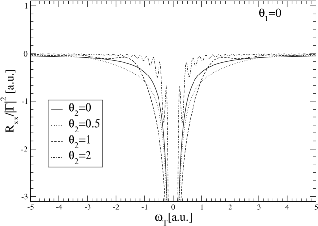
Figure 4.2: Plot of the resistance $R_{xx}/|\Gamma|^{2}$ given by Eq. (3.42) with the $g_{T}$ calculated in Eq. (4.35) for various values of $\theta_{2}$ at fixed $\theta_{1}=0$. The oscillations at large bias voltage becomes more and more pronounced with increasing $\theta_{2}$.

In Fig. 4.2 we plot $R_{xx}(\omega_{T})$ in the case that the inter-edge interaction is confined to the region of the constriction (i.e., we set $\theta_{1}=\theta_{3}=0$ and let $\theta_{2}$ assume several different values). Experimentally, $\theta_{2}$ can be increased by narrowing the constriction by the application of a gate potential. When $\theta_{2}=0$ there is no interaction and $R_{xx}$ diverges as $V_{T}^{\alpha-2}$ at low bias.

This low-bias behavior does not change upon increasing $\theta_{2}$ because the long time behavior is dominated by the exponent $\alpha$ which does not depend on $\theta_{2}$. At larger bias voltage, however, the plot of $R_{xx}$ shows oscillations, which become more pronounced with increasing $\theta_{2}$. We can express the period of these oscillations in terms of the physical parameters of the theory

$$\Delta V_{T}=\frac{h}{e^{*}t_{0}}=\frac{hc_{1}}{e^{*}d}\frac{\cosh 2\theta_{1}}{\cosh 2\theta_{2}}~{}.$$ (4.37)

The frequency of the oscillations increases with increasing $\theta_{2}$ as it is apparent in Fig. 4.2.

Making the conformal transformation (4.20) in Eqs. (4.28) and  (4.31), and substituting in Eqs. (4.24) and (4.33) we obtain, after lengthy calculations, the result for $g_{T}$ in the case of finite temperature

$$\begin{split}g_{T}(\omega_{T},T)=&4\frac{{e^{*}}^{2}|\Gamma|^{2}}{\hbar^{3}}\left(\frac{L_{2}}{2\pi c_{2}}\right)\left(\frac{L_{2}T}{2c_{2}}\right)^{\alpha-1}\frac{\sin\left(\frac{\pi\alpha}{2}\right)}{\sinh^{\alpha}(\pi Tt_{0})}\\ &\times\frac{\partial}{\partial\omega_{T}}\mathrm{Im}\left\{2^{\beta-1}\sinh^{\beta}(\pi Tt_{0})B\left(\frac{\beta}{2}-i\frac{\omega_{T}}{2\pi T},1-\beta\right)\right.\\ &+\frac{e^{i\omega_{T}t_{0}}}{\alpha-i\frac{\omega_{T}}{\pi T}}F\left(\alpha,1;1+\frac{\alpha}{2}-i\frac{\omega_{T}}{2\pi T};\frac{1}{1-e^{2\pi Tt_{0}}}\right)\\ &\left.-\frac{e^{i\omega_{T}t_{0}}}{\beta-i\frac{\omega_{T}}{\pi T}}F\left(\beta,1;1+\frac{\beta}{2}-i\frac{\omega_{T}}{2\pi T};\frac{1}{1-e^{2\pi Tt_{0}}}\right)\right\},\end{split}$$ (4.38)

where $F$ is the hypergeometric function of four arguments (also indicated as ${{}_{2}}F_{1}$) and $B$ the Euler beta function [21]. In the case $\theta_{1}=\theta_{2}$ we have $\alpha=\beta$, the first and third term cancel against each other and we recover Wen’s result.

In Fig. 4.3(a-d)

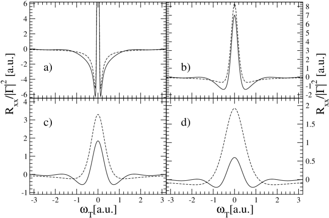
Figure 4.3: Plot of the differential resistance $R_{xx}/|\Gamma|^{2}$ vs. $\omega_{T}$ for a system with inter-edge interaction within the constriction (continuous line, $\theta_{1}=0$, $\theta_{2}=1$) and without inter-edge interaction (dashed line, $\theta_{1}=\theta_{2}=0$). The four curves correspond to different temperatures: $\pi Td/c_{1}=0.1$ (a), $0.5$ (b), $1$ (c), and $1.5$ (d).

we plot the differential resistance $R_{xx}$ vs. bias voltage for a system without inter-edge interaction (dashed line – $\theta_{2}=\theta_{1}=0)$ and with inter-edge interaction (solid line – $\theta_{1}=0$, $\theta_{2}=1$) for different values of $\pi dT/c_{1}=0.1,0.5,1$, and $1.5$. The non vanishing value of $\theta_{2}$ within the constriction induces oscillations in the $R_{xx}$ vs. $\omega_{T}$ relation with the same period as in the zero temperature case. However, we now have a maximum at zero bias voltage and two minima at finite bias voltage. This behavior is due to the fact that the temperature introduces a new energy scale. When the $e^{*}V>k_{B}T$ we are essentially in the zero temperature case and the resistance $R_{xx}$ decreases with decreasing bias voltage (see Fig. 4.2). But, when the $e^{*}V<k_{B}T$ the resistance turns around and begins to increase, reaching a maximum at zero bias. This behavior implies the presence of two minima located at bias voltages of the order of magnitude of $k_{B}T/e^{*}$: these are clearly seen in Fig. 4.3. The finite value of $R_{xx}$ at zero bias (independent of $V_{T}$ to first order) indicates that the constriction is behaving like an ohmic resistor in this regime, even though the resistance is strongly temperature-dependent.

The presence of a constriction adds another energy scale in the problem, associated with the inverse of the characteristic time $t_{0}$. For temperatures smaller than $\hbar/t_{0}$ the low bias behavior is dominated by the same exponent $\alpha$ (cf. Fig. 4.3 (a,b)) irrespective of whether the inter-edge interaction is present or not. When the temperature, instead, is greater than $\hbar/t_{0}$ the exponent $\beta$, which depends on the strength of the interaction within the constriction, controls the behavior of $R_{xx}$ (cf. Fig. 4.3(c,d)). As a consequence the minima at finite bias are generally deeper and shift to lower voltages.

The effect of the constriction depends quantitatively on both the inter-edge interaction parameter $\theta_{2}$ and the temperature. To appreciate this we plot in Fig. 4.4 the differential resistance $R_{xx}$ for different values of the inter-edge interaction and the temperature. More specifically we have plotted $R_{xx}$ without interactions ($\theta_{2}=\theta_{1}=0)$ and with interactions within the constriction ($\theta_{1}=0$, $\theta_{2}=0.2$) for $\pi dT/c_{1}=0.5,1,5$, and $10$.

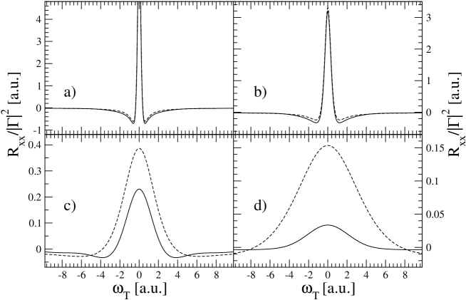
Figure 4.4: Plot of the differential resistance $R_{xx}/|\Gamma|^{2}$ vs. frequency with and without inter-edge interaction within the constriction. Solid line – $\theta_{1}=0$, $\theta_{2}=0.2$; Dashed line – $\theta_{1}=\theta_{2}=0$. Temperatures are $\pi dT/c_{1}=0.5$ (a), $1$ (b), $5$ (c), and $10$ (d).

We notice that the effect of the inter-edge interaction disappears at sufficiently low temperature, since it is always the long times exponent $\alpha$ that matters in that regime. The effect of the interaction shows up upon increasing the temperature above the crossover energy $\hbar/t_{0}$: the latter decreases with increasing $\theta_{2}$. Such a trend is clearly seen by comparing Figs. 4.3 and 4.4.

Chapter 5 Conclusions

In this chapter we compare our results with the theory of Wen and the measurements made by a group in Pisa showing that our model can explain some of the experimental features that are missed by the previously developed theories. After that we would like to discuss a few future research lines we can follow to further investigate these systems. Finally, we will state our conclusions.

5.1 Comparison with the experiments

The group of F. Beltram, V. Pellegrini, and S. Roddaro in Pisa has performed a series of measurements of the tunneling current due to quasi-particles tunneling between two edges belonging to the same Quantum Hall liquid [28]. In such a system, it is believed that the tunneling particles are the bulk quasi-particles with fractional charge. The results of Wen [14], and Kane and Fisher [16], predict that the tunneling conductance $G(T,V)$ must show a power law behavior both in voltage and in temperature,

$$G(0,V)\sim V^{\alpha};~{}~{}~{}~{}G(T,0)\sim T^{\alpha}$$ (5.1)

with the same exponent $\alpha$ determined by the filling factor

$$\alpha=2\nu-2,$$ (5.2)

and, because in these theories $\nu<1$, we have $\alpha<0$. The divergence of the conductance at very low bias is removed by the presence of a finite temperature, thus recovering a linear relation between the current and the voltage. Notice that the expected divergence is $G(0,V_{T})\to-\infty$ for $V_{T}\to 0$ then the effect of the temperature is to generate a zero bias maximum and two minima at finite bias. In the Fig. 5.1 we report the experimental data for the measure of the tunneling conductance [28]. The magnetic field is determined by fixing the filling factor to $\nu=1/3$ while the temperature is varied from $900$ mK to $30$ mK.

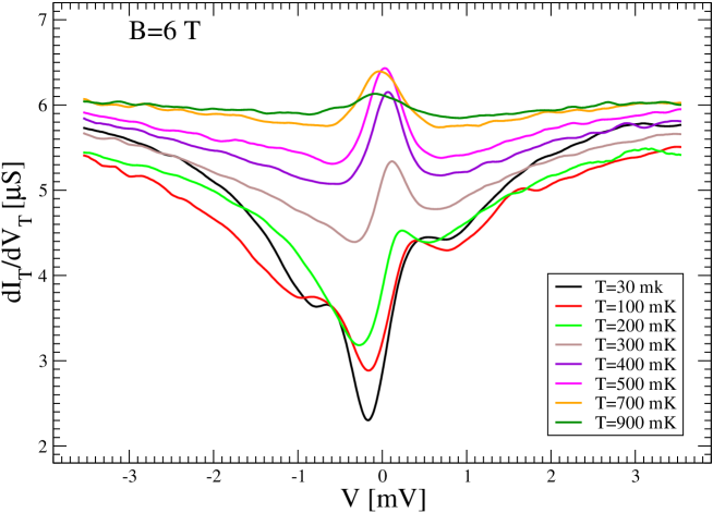
Figure 5.1: Plot of the differential conductance vs. the tunneling voltage for various temperatures at fixed magnetic field. The magnetic field and the experimental device fix $\nu=1/3$. Data from [28].

For high temperatures ($900-400$ mK), the central maximum is clearly seen. Also two deep minima are present. The general behavior is in qualitative good agreement with the expected theoretical behaviors (see Figs. 4.3 and 4.4). In this range of temperatures is also evident an asymmetry for the change of the sign of the tunneling potential. The origin of this asymmetry, which becomes more and more evident lowering the temperature, is not completely understood. There is the possibility, as discussions with the experimentalists have pointed out, that it can be an artifact of the experimental setup.

For lower temperatures ($400-30$ mK) the structure of the response function changes dramatically. The asymmetry becomes more evident, the central maximum disappears and a deep central minimum starts to develop. The origin of this central minimum is completely unknown and we expect that, if it is a genuine experimental result, we must plug in some other physical insights in our model to explain it.

For high temperatures and in the region of the central maximum, both our model and that of Wen can be compared with the experimental results. To do that we need to fit the experimental data with the theoretical curves to fix the free parameters: the translationally invariant interaction angle for Wen or the inside and outside mixing angles in our model. We choose to fit the data by using the least square minima technique. We have then looked at the minima of the sum of the squared difference of the experimental and theoretical curves to fix the parameters.

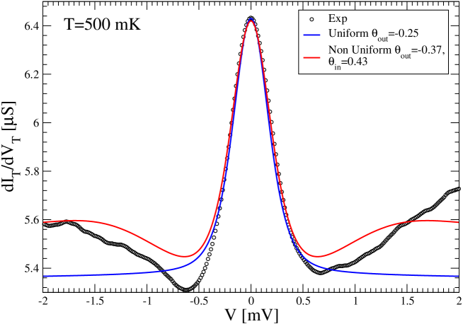
Figure 5.2: Plot of the experimental and theoretical results. The filling fraction $\nu=1/3$ and the temperature is fixed at $T=500$ mK. We have fixed the total amplitude of the theoretical curves because we do not known the value of the tunneling amplitude $|\Gamma|$ and partially removed the asymmetry by moving the central maximum at $V_{T}=0$.

In Fig. 5.2 we report the curves for the longitudinal conductance at $T=500~{}\mbox{mK}$ obtained after having determined the best fit parameters. From this plot is clearly seen that both the Wen’s theory and our model recover the structure of the central maximum. However the Wen’s theory does not recover neither the deep minima that are present at $|V|\sim 0.7$ mV nor the rise of the conductance at larger voltage.

We must point out that both the models predict either an attractive interaction in the region outside the constriction or a larger than $e^{*}=e/3$ quasi-particle charge. In fact we use as fit parameters the exponents of the tunneling conductance that tie together the quasi-particle charge $e^{*}$ and the outside interaction parameters in products like $(e^{*}/e)^{2}e^{-2\theta}$ and thus it is not possible to obtain from our fit direct measurements of the quasi-particle charge and of the mixing angle $\theta$, separately. Similar fits with the other experimental curves in the range $900$-$400$ mK have shown an increase of the term $(e^{*}/e)^{2}e^{-2\theta}$ when lowering the temperature. This dependence is not understood and is not predicted neither by our model nor by the theory of Wen. On the other hand it is not possible to extract from the experimental data a measure of the oscillation period as determined by the Eq. (4.37).

5.2 Perspectives

The results obtained so far allow us to consider some possible developments. In particular two arguments are attracting our attention. The first is the study of the tunneling in the edges of the Quantum Hall liquid in more detail. Indeed, when we have dealt with the problem of the tunneling into an edge, the problem of the fine structure of the edge was not considered at all. However has been pointed out by several authors that, even for the Laughlin state where $\nu=1/m$ with $m$ an odd integer, the edge can undergo a reconstruction [39, 40, 41, 42, 43] and acquire a complex structure. This reconstruction can affect the tunneling amplitudes by modifying the form of the quasi-particle creation and annihilation operators. One way to take into account this effect can be the inclusion in the tunneling Hamiltonian of other terms that describe the possibility that several species of quasi-particles can propagate into the edge. On this research line lies also the result of Eric Yang et al. [44]: The quasi-particle species that can undergo the tunneling between two edges depend on the separation width of the edges. In particular, if one considers the tunneling between two Laughlin states, when the edges are far-off the tunneling quasi-particles are the fractionally charged Laughlin quasi-particles. However, when the edges are close enough, other quasi-particles with different charges can do the tunneling. This research line can thus clarify the properties of the tunneling quasi-particles and their relation with the bulk quasi-particle.

The other argument we want to explore is a more detailed study of the effect of the constriction on the transport properties of the Quantum Hall bar. In fact we have not yet considered the possibility that the constriction, behaving like a semi-opaque barrier, has some tunneling resonances that will enhance the longitudinal conductance even when the magnetic field is not present. A possible way to attack this problem is to solve the quantum mechanical problem of the tunneling amplitudes of a constriction in a bidimensional system with zero magnetic field. We expect that these amplitudes depend on the energy of the impinging wave. When the magnetic field is not zero one can use the basis developed for the tunneling in the previous case to calculate the new transmission and reflection coefficients. This research can also open the way to a more accurate study of the dependence of the tunneling amplitude $\Gamma$ as a function of the physical parameters of the impinging quasi-particles.

5.3 Conclusions

The main subject of this thesis has been the study of the transport properties of a two dimensional electron gas in the presence of a high magnetic field. When the magnetic field is very strong the kinetic energy is quenched and the dynamics of the interacting electrons is produced by the commutation relations that appear among the density fluctuations as a result of the projection into the lowest Landau level. The phenomenology of the transport properties is shown in the Fig. 1.1. As we have discussed the transversal resistance $R_{xy}$ (also known as the Hall resistance) shows a series of plateaus at values $\sigma_{H}=\nu e^{2}/h$ where $\nu$ is either an integer or a rational number, while the longitudinal resistance $R_{xx}$ shows an alternation of vanishing regions and $\delta$-like peaks. This effect takes the name of Quantum Hall effect due to its connection with the Classical Hall effect.

To put our work in context, we have reviewed some of the theoretical approaches developed for the calculation of the response function of these systems. In this thesis we have chosen a hydrodynamical approach that allows us to treat $\nu$ as a free parameter without restricting ourselves to the case of $\nu$ being an integer or a rational number. This allows us to describe the dynamics of the quasi-particles as charge density fluctuations localized at the edges of the system. We have then developed the algebra to calculate the response functions by using these density fluctuations and its relations with the quasi-particle creation and annihilation operators. Our approach gives us the possibility to introduce, in a clear way, the interaction between the quasi-particles. We have shown in detail how our model can recover the linear relation between the filling factor $\nu$ and the transversal conductance.

This research started as a collaboration with the experimental group of F. Beltram, V. Pellegrini, and S. Roddaro in Pisa. The focus of the experimental research was the development of devices to detect and use the quasi-particle fractional charges. The experimental device used is reasonably well modelled by our idealized scheme (see Fig. 2.3). In studying this problem we had to face with two distinct problems. The first has been the possibility of tunneling between the edges and the other has regarded the possibility that the presence of the constriction can affect the transport properties.

We have thus decided to start by including the effect of the constriction directly in the Hamiltonian by considering the inter-edge interaction potential in a piece-wise form. The model in such a case can be easily solved. We have shown that the presence of a finite size constriction does not affect the low energy transport properties thus recovering the ideal relation between the conductance and the filling fraction. This result can be physically understood by observing that in the low energy limit, which corresponds to the long wavelength limit, the constriction becomes fully transparent and the transmission coefficient goes to $1$.

We have then discussed the possibility of tunneling between the edges inside the constriction. The presence of the constriction introduces a time scale, $t_{0}=d/c$. $t_{0}$ is the time a charge density wave needs to travel through the constriction. This time introduces then a separation in the behaviors for long and short (compared with $t_{0}$) times. We have discussed the fact that for short times the effect of the constriction becomes negligible. The low energy behavior is mainly determined by the long times behavior and this in turn is modified by the presence of the constriction. We have compared our work with the previously developed theory of Wen, who considers the case of tunneling between the edges in a translationally invariant system [13, 17, 14]. Many differences have been pointed out. In the regime of low bias voltage both theories predict the presence of a large central maximum. Near this maximum two deep minima develop. The structure of these minima differs in the two theories: in particular we predict that these minima must be much deeper than in the Wen’s theory. At larger bias voltages we predict the presence of small oscillations whose period $\delta V=h/e^{*}t_{0}$ allows a direct measure of the traveling time and of the quasi-particle charge.

We have then discussed the comparison of our result with some recent measurements of the tunneling conductance. We have shown that our model can explain some characteristics of the experimental results. Finally we have described possible future research lines.

Appendix A Proof of the commutation relations

In this appendix we discuss the commutation relations for the $\delta\rho_{\alpha}$ operators and show how to obtain it directly from the Lowest Landau Level projection and the hydrodynamical approximation. We consider separately the two cases of sharp and smooth edge.

A.1 Sharp edge case

Let us consider a single left edge. We imagine that the region $y<0$ is empty and there is a sharp wall at $y=0$. Then we have the condition on the wave number $k<0$. We suppose that the length scale of variation of the confining potential in the $y$ direction is smaller than $l$, hence we can neglect the states with $k$ around $0^{+}$ and approximate the number density with a $\theta$ function

$$n(k)=\nu\theta(-k).$$ (A.1)

Notice that the negative value of $k$ are given by the condition $y+kl^{2}=0$ which identifies the maximum of the gaussian packet in the LLL and then the position of the particle. There is a subtle point in this definition. The function $n(k)$ is discontinuous in $k=0$. We take $n(0)=\nu/2$. This assumption can be justified using the definition of the theta function such that $\theta(0)=1/2$. We define the transverse fluctuation

$$\delta\hat{\rho}(x)=\int\limits_{-\infty}^{\infty}dy\delta\hat{\rho}(x,y)$$ (A.2)

so we have the commutation relation between this new operators

$$\begin{split}[\delta\hat{\rho}(x),\delta\hat{\rho}(x^{\prime})]=&\int\limits_{-\infty}^{\infty}dy~{}dy^{\prime}~{}\sum_{k\not=h,m\not=l}\left(\hat{c}^{\dagger}_{k}\hat{c}_{l}\delta_{h,m}-\hat{c}^{\dagger}_{h}\hat{c}_{m}\delta_{k,l}\right)\\ &\times\varphi_{k}^{*}({\bf r})\varphi_{h}({\bf r})\varphi_{m}^{*}({\bf r}^{\prime})\varphi_{l}({\bf r}^{\prime})\\ =&\sum_{k\not=h}n(k)\int\limits_{-\infty}^{\infty}dy~{}dy^{\prime}~{}\left[\varphi_{k}^{*}({\bf r})\varphi_{h}({\bf r})\varphi_{h}^{*}({\bf r}^{\prime})\varphi_{k}({\bf r}^{\prime})\right.\\ &-\left.\varphi_{h}^{*}({\bf r})\varphi_{k}({\bf r})\varphi_{k}^{*}({\bf r}^{\prime})\varphi_{h}({\bf r}^{\prime})\right].\end{split}$$ (A.3)

If we use the expression for the function $\varphi_{k}({\bf r})$ in the LLL, in the given gauge,

$$\varphi_{k}(x,y)=\frac{1}{(\pi l^{2})^{\frac{1}{4}}}e^{-ikx}\exp\left[-\frac{(y+kl^{2})^{2}}{2l^{2}}\right]$$ (A.4)

we obtain

$$\int\limits_{-\infty}^{\infty}dy~{}\varphi_{k}^{*}(x,y)\varphi_{h}(x,y)=e^{-i(k-h)x}\exp\left[-\frac{(k-h)^{2}l^{2}}{4}\right]$$ (A.5)

and this allows us to calculate the commutator

$$\begin{split}[\delta\hat{\rho}(x),\delta\hat{\rho}(x^{\prime})]=&\sum_{k\not=h}n(k)\left(e^{-i(k-h)(x-x^{\prime})}-e^{i(k-h)(x-x^{\prime})}\right)\\ &\times\exp\left[-\frac{(k-h)^{2}l^{2}}{2}\right]\\ =&\sum_{q}e^{-iq(x-x^{\prime})}\exp\left[-\frac{q^{2}l^{2}}{2}\right]\sum_{h}\left(n(q+h)-n(h-q)\right)\\ =&-\sum_{q}\frac{\nu}{2\pi}qe^{-iq(x-x^{\prime})}\exp\left[-\frac{q^{2}l^{2}}{2}\right]\\ \stackrel{{\scriptstyle l\to 0}}{{=}}&-\frac{i\nu}{2\pi}\frac{d}{dx^{\prime}}\delta(x-x^{\prime}).\end{split}$$ (A.6)

The last expression has been obtained by observing that in the limit $l\to 0$ the gaussian may be approximated by a delta function. Notice also that $h$ is evaluated at $-q$ and $q$ which corresponds to $k=0$. This leads to a factor $1/2$ according to the definition of $n(0)$.

In the presence of two edges the derivation is similar but in this case the values allowed for the wave vectors in the expressions for the density fluctuations are different. Is such a case the Krönecker delta given by the commutator of the fermion operators cannot be fulfilled if the densities belong to different edges. Then the commutator is zero. Hence we obtain, if $\alpha,\beta\in\{L,R\}$ are the indexes of the edge,

$$\left[\delta\rho_{\alpha}(x),\delta\rho_{\beta}(x^{\prime})\right]=-\frac{i\nu}{2\pi}\frac{d}{dx}\delta(x-x^{\prime})\sigma_{\alpha,\beta}^{z}.$$ (A.7)

The appearance of the Pauli matrix $\sigma^{z}$ is justified by the different forms of the $n_{\alpha}(k)$ functions. In fact for the number densities we have, if $D$ is the distance between the edges,

$$n_{L}(k)=\left\{\begin{array}[]{l}\nu\theta(-k)\\ \nu/2~{}\mbox{if}~{}k=0\end{array}\right.$$ (A.10)

$$n_{R}(k)=\left\{\begin{array}[]{l}\nu\theta(k+D/l^{2})\\ \nu/2~{}\mbox{if}~{}k=-D/l^{2}\end{array}\right.$$ (A.13)

hence when we integrate over $h$ they assume a different sign

$$\int\limits_{-\infty}^{\infty}\frac{dh}{2\pi}\left[n_{L}(h+q)-n_{L}(h-q)\right]=-\frac{q}{2\pi},$$ (A.14)

$$\int\limits_{-\infty}^{\infty}\frac{dh}{2\pi}\left[n_{R}(h+q)-n_{R}(h-q)\right]=\frac{q}{2\pi}.$$ (A.15)

This completes the proof for the commutation relations in the case of a sharp edge.

A.2 Smooth edge case

Next we will consider the case of the smooth edge. In this case we rewrite the equation (2.19) in the form

$$[\delta\rho({\bf r}),\delta\rho({\bf r}^{\prime})]=\sum_{k,h}(n(k)-n(h))\varphi_{k}^{\dagger}({\bf r})\varphi_{k}({\bf r}^{\prime})\varphi_{h}^{\dagger}({\bf r}^{\prime})\varphi_{h}({\bf r})$$ (A.16)

and in the case of slowly varying density function we have

$$n(k)\simeq n(h)+(k-h)\partial_{k}n(k).$$ (A.17)

The commutator of the density fluctuations reads

$$[\delta\rho({\bf r}),\delta\rho({\bf r}^{\prime})] = \sum_{k,h}(k-h)\partial_{k}n(k)\varphi_{k}^{\dagger}({\bf r})\varphi_{k}({\bf r}^{\prime})\varphi_{l}^{\dagger}({\bf r}^{\prime})\varphi_{l}({\bf r})$$ (A.18)

$$\stackrel{{\scriptstyle l\to 0}}{{=}} -\frac{i}{2\pi l^{2}}\partial_{x}\partial_{k}n(k)\delta(y-y^{\prime})\delta(x-x^{\prime}).$$

Now by remembering that $n(k)=2\pi l^{2}\rho_{0}(y)$ and $kl^{2}=y~{}\Rightarrow dk=dy/l^{2}$ we have

$$[\delta\rho({\bf r}),\delta\rho({\bf r}^{\prime})]=-il^{2}\partial_{x}(\partial_{y}\rho_{0}(y))\delta(x-x^{\prime})\delta(y-y^{\prime})$$ (A.19)

and integrating over the edge we finally obtain

$$[\delta\rho_{\alpha}(x),\delta\rho_{\beta}(x^{\prime})] = \int_{\alpha}dy\int_{\beta}dy^{\prime}[\delta\rho({\bf r}),\delta\rho({\bf r}^{\prime})]$$ (A.20)

$$= -il^{2}\partial_{y}\sigma^{z}_{\alpha,\beta}\rho\delta(x-x^{\prime})$$

where $\rho_{0}(y)$ is the equilibrium density and $\rho$ is the bulk density. The apparition of the $\sigma^{z}$ matrix is justified by the order of the limit of integration in the edge: We have

$$\int_{L}dy~{}\partial_{y}\rho(y)=\rho(d)-\rho(0)=\rho,$$ (A.21)

$$\int_{R}dy~{}\partial_{y}\rho(y)=\rho(R+d)-\rho(R)=-\rho$$ (A.22)

if $d$ is the length over which the density goes from zero to the bulk value (supposed for simplicity equal for the two edges). The final observation that $\nu=2\pi l^{2}\rho_{0}$ completes the proof.

Appendix B Properties of the eigenvalues problem

In this appendix we want to study some analytical properties of the equation (2.34). First of all let us define the operators

$$M_{\alpha,\beta} = i\sigma_{\alpha,\beta}^{z}\partial_{x},$$ (B.1)

$$H_{\alpha,\beta} = \frac{\nu}{2\pi}\int\limits_{-\infty}^{\infty}dx~{}\partial_{x}V_{\alpha,\beta}(x,x^{\prime})\partial_{x^{\prime}}.$$ (B.2)

With this definition we rewrite the equation of motion (2.34) in the compact form

$$\omega M\varphi=H\varphi.$$ (B.3)

It is easy to see that $H$ and $M$ are hermitian operators and we request that $H$ is positive definite (this will assure the stability of the physical system).

Let us define the auxiliary function

$$\Psi=H^{\frac{1}{2}}\varphi$$ (B.4)

which is a solution of the equation

$$\frac{1}{\omega}\Psi=\left(H^{-\frac{1}{2}}MH^{-\frac{1}{2}}\right)\Psi=\tilde{M}\Psi$$ (B.5)

if $\varphi$ is a solution of (2.34). Because $\tilde{M}$ is an hermitian operator we have the results:

1. the set $\{\Psi\}$ of solutions forms a complete base of the Hilbert space,

2. the orthonormality condition is

   $$\sum_{\alpha}\int dx\Psi_{n,\alpha}^{*}(x)\Psi_{m,\alpha}(x)=\delta_{n,m},$$ (B.6)

3. the completeness relation

   $$\sum_{n}\Psi_{n,\alpha}(x)\Psi_{m,\beta}^{*}(x^{\prime})=\delta_{\alpha,\beta}\delta(x-x^{\prime}).$$ (B.7)

Because there is a one-to-one relation between $\varphi$ and $\Psi$ we have the following properties of the solutions of equation (2.34):

1. the solutions $\varphi$ form a complete base of the Hilbert space,

2. they are orthogonal with respect to the scalar product

   $$(\varphi_{n},\varphi_{m})=\sum_{\alpha}\int dx~{}\omega_{n}\varphi_{n,\alpha}^{*}(x)M_{\alpha,\beta}\varphi_{m,\beta}(x),$$ (B.8)

3. they satisfy the completeness relation

   $$-i\sum_{n}\omega_{n}\varphi_{n,\alpha}(x)\varphi_{n,\beta}^{*}(x^{\prime})s_{\beta}\partial_{x}=\delta_{\alpha,\beta}\delta(x-x^{\prime}).$$ (B.9)

We obtain the relations reported in the text if we normalize the functions $\varphi_{n}$ as $\varphi_{n}/\sqrt{|\omega_{n}|}$.

Now we want discuss the degeneracy of the eigenvalues of the equation (2.34):

• If $\varphi_{n,\alpha}(x)$ is a solution with given eigenvalue $\omega_{n}$ then the function $\varphi_{n,\alpha}^{*}(x)$ is also a solution with eigenvalue $\omega_{-n}=-\omega_{n}$.

• If $\varphi_{m,\alpha}(x)$ is a solution with given eigenvalue $\omega_{m}$ then the function $\sigma_{\alpha,\beta}^{x}\varphi_{m,\beta}(x)$ is also a solution with eigenvalue $-\omega_{m}$.

Then we have that if $\varphi_{m,\alpha}(x)$ is a solution then $\sigma_{\alpha,\beta}^{x}\varphi_{m,\beta}^{*}(x)$ is still a solution with the same eigenvalue thus the solutions of problem (2.34) are doubly degenerate.

Appendix C Landauer-Büttiker transport formalism

In this appendix we want to discuss briefly the Landauer-Büttiker formalism for the transport in one-dimensional system and its application to the Quantum Hall edge transport [45].

We will discuss before the case of the Integer Quantum Hall phase where many edge states are present. Every such state is a possible channel for the current transport. In the clean case, when there is not tunneling between different edges, in a six probes geometry similar to the one showed in the Fig. 1.3, we can write the balance equations

$$\left(\begin{array}[]{c}I_{1}\\ I_{4}\\ I_{2}\\ I_{3}\\ I_{5}\\ I_{6}\end{array}\right)=\frac{e^{2}}{h}(N+1)\left(\begin{array}[]{cccccc}1&0&0&0&0&-1\\ 0&1&0&-1&0&0\\ -1&0&1&0&0&0\\ 0&0&-1&1&0&0\\ 0&-1&0&0&1&0\\ 0&0&0&0&-1&1\end{array}\right)\left(\begin{array}[]{c}V_{1}\\ V_{4}\\ V_{2}\\ V_{3}\\ V_{5}\\ V_{6}\end{array}\right)$$ (C.1)

where we have assumed that the current in the $i$-th terminal is determined only by its potential and the potential of the contact directly “down-stream” with respect to the versus of propagation of the edge which leaves the terminal. Notice also that we have ordered differently the reservoir to have a direct comparison with the matrix conductance given by the Eq. (3.41). We have also considered the possibility that $N+1$ propagation channels are present. To solve this set of equations one fixes the current of the terminal $2,~{}3,~{}5$ and $6$ to zero then the total current is given by $I=I_{1}=-I_{4}$. We fix also the potential of the terminal $4$ to zero. We obtain, by defining $\sigma_{i,j}=I/(V_{i}-V_{j})$

$$\begin{split}&\sigma_{2,3}=\sigma_{5,6}=0,\\ &\sigma_{2,5}=\sigma_{2,6}=\sigma_{3,5}=\sigma_{3,6}=\frac{e^{2}}{h}(N+1).\end{split}$$ (C.2)

It is possible to generalize such approach to the case of the FQHE by substituting the number of possible channels $N+1$ with the filling fraction $\nu$.

It is also possible to consider the effect of the tunneling between two edges. We model this tunneling by defining a transmission $T$ and a reflection $R$ probability. The reflection coefficient is given by the probability that a particle moving from $2$ to $3$ or from $5$ to $6$ tunnels to the other edge. We have

$$\left(\begin{array}[]{c}I_{1}\\ I_{4}\\ I_{2}\\ I_{3}\\ I_{5}\\ I_{6}\end{array}\right)=\frac{e^{2}}{h}\nu\left(\begin{array}[]{cccccc}1&0&0&0&0&-1\\ 0&1&0&-1&0&0\\ -1&0&1&0&0&0\\ 0&0&-T&1&-R&0\\ 0&-1&0&0&1&0\\ 0&0&-R&0&-T&1\end{array}\right)\left(\begin{array}[]{c}V_{1}\\ V_{4}\\ V_{2}\\ V_{3}\\ V_{5}\\ V_{6}\end{array}\right).$$ (C.3)

Notice that the gauge invariance and the current conservation require that $R+T=1$. We can solve this system with the same requirements for the setup of the currents and voltages to obtain the conductance matrix in this case. In the limit $R\to 0$ we recover the previous result.

A more complex matrix can be obtained if one considers the reservoirs coupled as we have discussed in Eq. (3.41). If we consider the non interacting case $u=1,~{}v=0$ from the Eq. (3.41) we have

$$G_{ij}=\frac{e^{2}}{h}\nu\left(\begin{array}[]{cccccc}1&0&0&0&0&-1\\ 0&1&0&-1&0&0\\ -1&0&1&0&0&0\\ 0&0&-1+\delta g_{21}&1&\delta g_{23}&0\\ 0&-1&0&0&1&0\\ 0&0&\delta g_{41}&0&-1+\delta g_{43}&1\end{array}\right).$$ (C.4)

The gauge invariance and the conservation of the current fix the allowed values of the conductances $\delta g_{21}$, $\delta g_{23}$, $\delta g_{41}$, $\delta g_{43}$: we have then

$$R=\delta g_{21}=\delta g_{43}=-\delta g_{41}=-\delta g_{23}=i\lim_{\omega\to 0}\frac{\tilde{M}_{T}(\omega)}{\omega}e^{-2\theta}.$$ (C.5)

The presence of the constriction couples all the edges and we must solve the linear problem given by the Eq. (3.41). In such case it is not possible to define a single reflection coefficient and express the solution only in terms of it.

Appendix D Evaluation of integrals

In this appendix we provide a few details concerning the evaluation of the integral occurring in the calculation of the Fourier transform of the response function $G_{-}(t)$. In the zero temperature case, we must evaluate an integral of the form

$$\int\limits_{t_{0}}^{\infty}dt(\delta\pm it)^{-\alpha}e^{i\omega t}$$ (D.1)

where $\alpha$ is a positive real number. To do this we go in the complex plane of the variable $t$ and consider, for positive frequency $\omega$, an integration path as the one shown in Fig. D.1.

Figure D.1: The integration path used to evaluate the integral (D.1) when the frequency is positive. A similar path, closed in the lower plane, is used in the case $\omega<0$.

A specular path in the lower half plane must be used for negative frequency. We observe that the integrand function has no poles in the complex half-plane of $t$ with a positive real part. Hence the integral on the whole path is zero. The integral on the arc vanishes by letting the radius go to infinity.

As a result we get

$$\int\limits_{t_{0}}^{\infty}dt(\delta\pm it)^{-\alpha}e^{i\omega t}\stackrel{{\scriptstyle\delta\to 0}}{{=}}i(\mp 1)^{-\alpha}\omega^{\alpha-1}\Gamma(1-\alpha,-i\omega t_{0}).$$ (D.2)

The case $t_{0}=0$ can be carried out by calculating the convolution product between the Fourier transform of the $\Theta(t)$ function and the integral

$$\begin{split}\int\limits_{-\infty}^{\infty}dt(\delta\pm it)^{-\alpha}e^{i\omega t}=&2\sin(\pi\alpha)e^{i\frac{\pi}{2}\alpha}|\omega|^{-1-\alpha}\\ &\times\Gamma(1+\alpha)(\mp 1)^{-1-\alpha},\end{split}$$ (D.3)

obtained by cutting the complex plane along the imaginary axis, starting from $t=\pm i\delta$ as is shown in the Fig. D.2 when the singularity is located in the upper plane and for positive frequency. Similar paths were used in the other cases.

Figure D.2: The integration path used for the evaluation of the integral  (D.3) when the frequency is positive. A specular path with respect to the real axis is used when the singularity is located in the lower plane. Similar paths were used in the other cases.

In the finite temperature case, we need to calculate the integral

$$\int\limits_{t_{0}}^{\infty}dt~{}e^{i\omega t}\frac{{(\pi T)}^{\alpha}}{\sinh(\pi Tt)^{\alpha}}.$$ (D.4)

One can easily obtain the result reported in the text by means of the substitution $s=e^{-2\pi Tt}$ which reduces the above integral to the definition of the hypergeometric $F$ function of four arguments [21, 46]. The integral with $t_{0}=0$ can be easily obtained in the limit $t_{0}\to 0$ by using the corresponding limiting expression of the hypergeometric function $F$ in terms of the Euler beta function.

References

- von Klitzing et al. [1980] K. von Klitzing, G. Dorda, and M. Pepper, Phys. Rev. Lett. 45, 494 (1980).
- Tsui et al. [1982] D. C. Tsui, H. L. Stormer, and A. C. Gossard, Phys. Rev. Lett. 48, 1559 (1982).
- Laughlin [1983] R. B. Laughlin, Phys. Rev. Lett. 50, 1395 (1983).
- de Picciotto et al. [1997] R. de Picciotto, M. Reznikov, M. Heiblum, V. Umansky, G. Bunin, and D. Mahalu, Nature 389, 162 (1997).
- Griffiths et al. [2000] T. Griffiths, E. Comforti, H. Heiblum, A. Stern, and V. Umansky, Phys. Rev. Lett. 85, 3918 (2000).
- Comforti et al. [2002] E. Comforti, Y. C. Chung, M. Heiblum, V. Umansky, and D. Mahalu, Nature 416, 515 (2002).
- Maasilta and Goldman [1997] I. J. Maasilta and V. I. Goldman, Phys. Rev. B 55, 4081 (1997).
- Jain [1989] J. K. Jain, Phys. Rev. Lett. 63, 199 (1989).
- Heinonen [1998] O. Heinonen, ed., Composite Fermions (World Scientific, Singapore, 1998).
- Stormer [1992] H. L. Stormer, Physica B 177, 401 (1992).
- Halperin [1982] B. I. Halperin, Phys. Rev. B 25, 2185 (1982).
- Haldane [1981] F. D. M. Haldane, J. Phys. C: Cond. Mat. 14, 2585 (1981).
- Wen [1990] X. G. Wen, Phys. Rev. B 41, 12838 (1990).
- Wen [1991a] X. G. Wen, Phys. Rev. B 44, 5708 (1991a).
- de Chamon et al. [1997] C. de Chamon, D. Freed, S. Kivelson, S. Sondhi, and X. Wen, Phys. Rev. B 55, 2331 (1997).
- Kane and Fisher [1995] C. L. Kane and M. P. A. Fisher, Phys. Rev. B 51, 13449 (1995).
- Wen [1991b] X. G. Wen, Phys. Rev. B 43, 11025 (1991b).
- Wen [1995] X. G. Wen, Adv. Phys. 44, 405 (1995).
- Comtet et al. [1999] A. Comtet, T. Jolicoeur, S. Ouvry, and F. David, eds., Topological aspects of low dimensional systems, vol. 69 of Les Houches-Ecole d’Ete de Physique Teorique (Springer-Verlag, New York, 1999), see S. M. Girvin, chapt. 2, The Quantum Hall Effect: Novel Excitations and Broken Symmetries.
- Landau [1930] L. D. Landau, Z. Physik 64, 629 (1930).
- Abramowitz and Stegun [1964] M. Abramowitz and I. A. Stegun, eds., Handbook of mathematical functions (National Bureau of Standards, Washington, D.C., 1964).
- Das Sarma and Pinczuck [1996] S. Das Sarma and A. Pinczuck, eds., Perspectives in Quantum Hall effect (Wiley, New York, 1996).
- Chakraborty and Pietilainen [1988] T. Chakraborty and P. Pietilainen, The Fractional Quantum Hall Effect: Properties of an Incompressible Quantum Fluid (Springer-Verlag, New York, 1988).
- Prange and Girvin [1990] R. E. Prange and S. M. Girvin, eds., The Quantum Hall Effect (Springer-Verlag, New York, 1990).
- Saminadayar et al. [1997] L. Saminadayar, D. C. Glattli, Y. Jin, and B. Etienne, Phys. Rev. Lett. 79, 2526 (1997).
- Haldane [1983] F. D. M. Haldane, Phys. Rev. Lett. 51, 605 (1983).
- Halperin [1984] B. I. Halperin, Phys. Rev. Lett. 52, 1583 (1984).
- Roddaro et al. [2003] S. Roddaro, V. Pellegrini, F. Beltram, G. Biasiol, L. Sorba, R. Raimondi, and G. Vignale, Phys. Rev. Lett. 90, 046805 (2003).
- Conti and Vignale [1998a] S. Conti and G. Vignale, J. Phys.: Condens. Matter 57, 3781 (1998a).
- Conti and Vignale [1998b] S. Conti and G. Vignale, Physica E 1, 101 (1998b).
- D’Agosta et al. [2003] R. D’Agosta, R. Raimondi, and G. Vignale (2003), cond-mat/0302201 submitted to Phys. Rev. B.
- Mahan [1981] G. D. Mahan, Many-Particle Physics (Plenum, New York, 1981).
- Girvin et al. [1986] S. M. Girvin, A. H. MacDonald, and P. M. Platzman, Phys. Rev. B 33, 2481 (1986).
- Aleiner and Glazman [1994] I. B. Aleiner and L. I. Glazman, Phys. Rev. Lett. 74, 2935 (1994).
- Oreg and Finkel’stein [1995] Y. Oreg and A. M. Finkel’stein, Phys. Rev. Lett. 74, 3668 (1995).
- Chklovskii and Halperin [1998] D. B. Chklovskii and B. I. Halperin, Phys. Rev. B 57, 3781 (1998), when is replaced by we find the result obtained in this paper.
- Luther and Peschel [1974] A. Luther and I. J. Peschel, Phys. Rev. B 9, 2911 (1974).
- Shankar [1990] R. Shankar, J. Mod. Phys. B 4, 2371 (1990).
- Chklovskii et al. [1992] D. B. Chklovskii, B. I. Shklovskii, and L. I. Glazman, Phys. Rev. B 46, 4026 (1992).
- de Chamon and Wen [1994] C. de Chamon and X. G. Wen, Phys. Rev. B 49, 8227 (1994).
- Wan et al. [2002] X. Wan, K. Yang, and E. H. Rezayi, Phys. Rev. Lett. 88, 056802 (2002).
- Rosenow and Halperin [2002] B. Rosenow and B. I. Halperin, Phys. Rev. Lett. 88, 096494 (2002).
- Joglekar et al. [2003] Y. N. Joglekar, H. K. Nguyen, and G. Murthy (2003), cond-mat/0303359v2.
- Eric Yang et al. [2002] S.-R. Eric Yang, S. Mitra, M. P. A. Fisher, and A. H. MacDonald (2002), cond-mat/0212170.
- Büttiker [1988] M. Büttiker, Phys. Rev. B 38, 9375 (1988).
- Gradshteyn and Ryzhik [1965] I. S. Gradshteyn and I. M. Ryzhik, Table of Integrals, Series and Products (Academic Press, New York, 1965).