Self-Consistent Modification To The Electron Density Of States Due To Electron-Phonon Coupling In Metals

Abstract

The ”standard” theory of a normal metal consists of an effective electron band which interacts with phonons and impurities. The effects due to the electron-phonon interaction are often delineated within the Migdal approximation; the properties of many simple metals are reasonably well described with such a description. On the other hand, if the electron-phonon interaction is sufficiently strong, a polaron approach is more appropriate. The purpose of this paper is to examine to what degree the Migdal approximation is self-consistent, as the coupling strength increases. We find that changes in the electron density of states become significant for very large values of the coupling strength; however, there is no critical value, nor even a crossover regime where the Migdal approximation has become inconsistent. Moreover, the extent to which the electron band collapses is strongly dependent on the detailed characteristics of the phonon spectrum.

I INTRODUCTION

The Migdal approximation for the electron self energy due to the electron-phonon interaction consists of neglecting vertex corrections. This procedure was first justified by Migdal migdal58 based on an approximate treatment of the first-order vertex correction. He found that the correction to the bare vertex is of order $O(\lambda{\omega_{D}\over\epsilon_{F}})$, where $\lambda$ is the dimensionless electron-phonon coupling constant, $\omega_{D}$ is the typical phonon frequency, and $\epsilon_{F}$ is the electron Fermi energy. If we ignore the factor of $\lambda$ note1 , then the ratio $\omega_{D}/\epsilon_{F}$ is generally very small in a metal.

Subsequently, Engelsberg and Schrieffer engelsberg63 performed numerical calculations of the self energy and spectral function, based on the Migdal approximation note2 . The result is found in several reviews and texts allen82 ; nakajima80 , and we quote here the main results. The electron self energy is given by a frequency dependent, momentum independent function,

$$\Sigma(\omega+i\delta)=\int_{0}^{\infty}d\nu\,\,\alpha^{2}F(\nu)\biggl{[}\,\,-2\pi i(n(\nu)+1/2)+$$

$$\psi\bigl{(}{1\over 2}+i{\nu-\omega\over 2\pi T}\bigr{)}-\psi\bigl{(}{1\over 2}-i{\nu+\omega\over 2\pi T}\bigr{)}\,\,\biggr{]}$$ (1)

where $\psi(x)$ is the digamma function abramowitz64 ; allen82 and the entire expression has been written for a frequency just above the real axis, $\omega+i\delta$. In Eq. (1) $n(\nu)$ is the bose function, and $\alpha^{2}F(\nu)$ is the electron-phonon spectral function. A truly self-consistent approach would require, amongst other things, a self-consistent correction to the phonon spectrum, due to the interaction with electrons. Migdal estimated this correction, and found that the phonon frequencies are renormalized, and an instability is encountered as the bare coupling strength increases. However, we are adopting a more phenomenological approach here. The common practice scalapino69 is to take information concerning the phonons from experiment as input into the theory for the electrons. The justification for this comes from experiment, where well-defined phonons are observed in neutron scattering experiments brockhouse62 , for example. Since these are used in the theory for the electron properties, it would be incorrect to compute renormalizations for the phonons. We follow this philosophy in everything that follows note3 .

Nonetheless, Eq. (1) was obtained with a number of other simplifying assumptions and approximations. In particular the self energy of the electron is determined by an infinite set of diagrams in which phonon lines do not cross; these can be summarized by the diagram in Fig. 1, where the full electron Green function, $G({\bf k},\omega+i\delta)\equiv 1/(\omega+i\delta-\epsilon_{\bf k}-\Sigma({\bf k},\omega+i\delta))$, is required, and of course depends on the very self energy that we are trying to calculate. Yet Eq. (1) shows no sign of self-consistency. The reason was noted already in Ref. migdal58 and arises because the bandwidth is assumed to be essentially infinite compared to the typical phonon energy. Then, the nested diagrams which arise from iterating the equation in Fig. 1 all contribute zero, and the same result is obtained by simply replacing the full electron Green function in the figure with the non-interacting Green function.

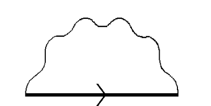
Figure 1: Diagram for the electron self energy. Note that the self-consistent electron Green function (heavy solid line) is used in this calculation.

Engelsberg and Schrieffer engelsberg63 relaxed the assumption of infinite bandwidth mitrovic83 , but used realistic values for the phonon frequency and Fermi energy for materials known at that time. They found only very small effects. More recently, Alexandrov et al. alexandrov87 readdressed the question of the impact of a finite (i.e. not infinite) bandwidth on the electron properties, and adopted much more extreme values of the ratio of the typical phonon frequency to Fermi energy, $\omega_{D}/\epsilon_{F}$ (referred to hereafter as the frequency ratio). They concluded that the Migdal approximation breaks down for coupling strengths that exceed unity.

In this paper we wish to assess this conclusion, by examining the effect of a more realistic phonon spectral function. Alexandrov et al. alexandrov87 used an Einstein spectrum to simplify the calculation. This spectrum is, of course, singular, and it is perhaps not too surprising if singular behaviour in the electron properties results. We will first outline the problem as posed by Alexandrov et al. and demonstrate that singular behaviour exists for any coupling strength. We argue that this behaviour does not necessarily invalidate the calculation, as tacitly assumed in Ref. alexandrov87 . Instead those authors properly focused on the more global behaviour of the electron density of states (EDOS), as a function of increased coupling strength. We examine in much more detail this global behaviour as a function of the parameters in the problem, so that a more quantitative assessment of the breakdown can be obtained. In particular we examine the dependency of the band collapse on the frequency ratio, the electron-phonon coupling strength, the presence of a secondary band, the shape of the bare band (Lorentzian versus square), and finally, the shape of the electron phonon spectral function, $\alpha^{2}F(\nu)$. For convenience $\alpha^{2}F(\nu)$ is modified from an Einstein spectrum to a Lorentzian. In this way a single parameter (the width of the spectrum) controls its shape. We find that there is no clear transition or even crossover to a regime where the Migdal approximation has become inconsistent. Nonetheless, this conclusion is not meant to imply that this calculation shows that the Migdal approximation is accurate in the intermediate or strong coupling regime. As will be summarized in the final section, other work suggests that this is not the case. Our calculation merely shows that within the Migdal framework, a signal of this potential breakdown does not occur, if a broad phonon spectrum is used.

II THE SELF-CONSISTENT MIGDAL APPROXIMATION

The self-consistent Migdal approximation results in the following equation for the electron self energy $\Sigma(\omega+i\delta)$:

$$\Sigma(\omega+i\delta)=\int_{0}^{\infty}d\nu\,\alpha^{2}F(\nu)\,\hskip 101.17755pt$$

$$\int_{-\infty}^{\infty}d\omega^{\prime}\,\frac{N(\omega^{\prime})}{N_{\circ}(0)}\biggl{[}\frac{n(\nu)+f(-\omega^{\prime})}{\omega+i\delta-\nu-\omega^{\prime}}+\frac{n(\nu)+f(\omega^{\prime})}{\omega+i\delta+\nu-\omega^{\prime}}\biggr{]}$$ (2)

where

$$N(\omega)=\int_{-\infty}^{\infty}d\epsilon\,N_{\circ}(\epsilon)A(\epsilon,\omega).$$ (3)

In these equations $f(\omega)$ and $n(\nu)$ are the Fermi and Bose distribution functions, respectively, $N_{\circ}(\epsilon)$ is the non-interacting (bare) electron density of states, and $N(\omega)$ is the self-consistently calculated electron density of states. The electron spectral function, $A(\epsilon,\omega)$ is given by

$$A(\epsilon,\omega)\equiv-{1\over\pi}{\rm Im}G(\epsilon,\omega+i\delta),$$ (4)

where the single electron Green function is given by

$$G(\epsilon,\omega+i\delta)={1\over\omega+i\delta-\epsilon-\Sigma(\omega+i\delta)}.$$ (5)

Notice that we have tacitly assumed that the electron self energy is independent of momentum (i.e. independent of $\epsilon$). The arguments that justify this simplification are provided, for example, in Ref. allen82 .

In Eq. (3), if $N_{\circ}(\epsilon)$ is taken to be a constant ($=N_{\circ}(0)$), extending over all energies, then using the fact that $\Sigma$ is independent of momentum (i.e. $\epsilon$), we obtain $N(\omega)=N_{\circ}(0)$. Thus, the standard approximation, that the Fermi energy and bandwidth are large energies compared to the phonon energy (so that we can neglect the former and simply integrate from $-\infty$ to $\infty$) leads to an electron density of states which is unmodified by the electron-phonon interaction. This is true even though the self energy has a non-trivial frequency dependence note4 . When a more realistic bare electron density of states is used, then Eq. (3) leads to an altered EDOS. For example, with $N_{\circ}(\epsilon)=N_{\circ}(0)\theta(D/2-|\epsilon|)$, i.e. a constant over a limited energy range, Eq. (3) gives

$${N(\omega)\over N_{\circ}(0)}=\frac{1}{\pi}\biggl{[}\arctan\bigl{(}\frac{D/2+Re\Sigma(\omega+i\delta)-\omega}{|Im\Sigma(\omega+i\delta)|}\bigr{)}+$$

$$\arctan\bigl{(}\frac{D/2-Re\Sigma(\omega+i\delta)+\omega}{|Im\Sigma(\omega+i\delta)|}\bigr{)}\biggr{]}.$$ (6)

If a Lorentzian form is used the bare density of states is given by

$$N_{\circ}(\epsilon)=N_{\circ}(0){(D/2)^{2}\over\epsilon^{2}+(D/2)^{2}}.$$ (7)

In either case $N_{\circ}(0)$ is the density of states at the Fermi level and $D$ is the full bandwidth, defined in an obvious way in the case of the constant case, and as the full width at half maximum in the Lorentzian case. For this latter case, Eq. (3) gives alexandrov87

$${N(\omega)\over N_{\circ}(0)}=\frac{D/2(D/2+|{\rm Im}\Sigma(\omega+i\delta)|)}{({\rm Re}\Sigma(\omega+i\delta)-\omega)^{2}+(|{\rm Im}\Sigma(\omega+i\delta)|+D/2)^{2}}.$$ (8)

Eq. (8) or (6) is required to self-consistently calculate the electron self energy given by Eq. (2). In what follows we further simplify the calculation by adopting $T=0$, as in Ref. alexandrov87 . This simplifies Eq. (2) since $f(\omega)\rightarrow\theta(-\omega)$ and $n(\nu)\rightarrow 0$ in this limit. Also, we will adopt particle-hole symmetry throughout this paper. The final equations, separated out into their real and imaginary parts, are given by

$${\rm Re}\Sigma(\omega+i\delta)=\hskip 180.67499pt$$

$$\int_{0}^{\infty}\,d\nu\,\alpha^{2}F(\nu)\biggl{[}\int_{0}^{\infty}d\omega^{\prime}\,{N(\omega^{\prime})\over N_{\circ}(0)}{2\omega\over\omega^{2}-(\nu+\omega^{\prime})^{2}}\biggr{]}$$ (9)

and

$${\rm Im}\Sigma(\omega+i\delta)=-\pi\int_{0}^{\infty}\,d\nu\,\alpha^{2}F(\nu)\biggl{[}{N(\omega-\nu)\over N_{\circ}(0)}\theta(\omega-\nu)+$$

$${N(\omega+\nu)\over N_{\circ}(0)}(1-\theta(\omega+\nu))\biggr{]}.\hskip 36.135pt$$ (10)

As mentioned in the introduction, the primary purpose of this paper is to explore the consequences of a non-singular phonon spectrum. For simplicity we will adopt a Lorentzian spectrum for the phonons, given by

$$\alpha^{2}F(\nu)=\hskip 180.67499pt$$

$$\frac{\lambda^{\prime}\omega_{E}}{2\pi}\biggl{(}\frac{\delta}{(\nu-\omega_{E})^{2}+\delta^{2}}-\frac{\delta}{\eta^{2}+\delta^{2}}\biggr{)}\theta(\eta-|\omega_{E}-\nu|),$$ (11)

where the subtracted term ensures that the spectrum is continuous everywhere, particularly at the endpoints, and $\eta$ is the full width of the spectral function (less than $\omega_{E}$). As the parameter $\delta$ approaches zero, this spectrum approaches an Einstein spectrum centered at $\omega=\omega_{E}$, and $\lambda^{\prime}\rightarrow\lambda$. Fig. 2 shows several spectra for different values of $\delta$.

Figure 2: The sequence of phonon spectral functions used to model broadening. The curves are truncated Lorentzians as described in the text with widths as labelled.

As a technical aside, simplifications occur for the Einstein spectrum, where $\alpha^{2}F(\nu)={\lambda\omega_{E}\over 2}\delta(\nu-\omega_{E})$. As is apparent from Eq. (10), ${\rm Im}\Sigma(\omega+i\delta)$ becomes simply related to the self-consistent EDOS. The real part of the self energy becomes singular, as is evident when Eq. (9) is rewritten for an Einstein phonon spectrum as

$${\rm Re}\Sigma(\omega+i\delta)=\hskip 180.67499pt$$

$${\lambda\omega_{E}\over 2}\biggl{[}\int_{0}^{\infty}d\omega^{\prime}\,\bigl{(}{(N(\omega^{\prime})-N(\omega-\omega_{E})\over N_{\circ}(0)}\bigr{)}{2\omega\over\omega^{2}-(\omega_{E}+\omega^{\prime})^{2}}$$

$$+{N(\omega-\omega_{E})\over N_{\circ}(0)}\,{\rm ln}|{\omega-\omega_{E}\over\omega+\omega_{E}}|\biggr{]},\hskip 36.135pt$$ (12)

and the logarithmic singularity is now explicit. Using an EDOS that is constant with infinite bandwidth gives zero for the $\omega^{\prime}$ integral in Eq. (12), and we recover the ‘standard’ result engelsberg63 for the electron self energy.

III RESULTS

Einstein phonon spectrum

It is clear from the discussion in the previous section that there is a simple scaling relation amongst the energies in the problem. Nonetheless we will use real units, and the reader can scale the results to other energy scales, if so desired. We begin with $\omega_{E}=10$ meV, and use a bandwidth 10X this amount, i.e. $D=10\omega_{E}=100$ meV. For definiteness we use $\lambda=2$, which is considered very strong coupling (Pb, for example, has $\lambda\approx 1.5$), and $N_{\circ}(0)=1/D$. In Fig. 3 we plot the (a) real and (b) imaginary parts of the electron self energy as a function of frequency for these parameters. We adopt a Lorentzian shape for the bare EDOS. Three curves are shown; one is for the standard theory, where an infinitely wide band with constant density of states is assumed, the second is for the non-self-consistent result, where the bare EDOS ($N_{\circ}(\omega)$) is substituted for $N(\omega)$ on the right hand side of Eqs. (12,10), and the third represents the full self-consistent solution to these same equations, using Eq. (8) in addition.

Figure 3: The (a) real and (b) imaginary parts of the electron self energy as a function of frequency, using an Einstein spectrum for the phonons and a Lorentzian for the bare EDOS, with $\omega_{E}/D=1/10$. The curves are computed with $\omega_{E}=10$ meV, and $\lambda=2$. The non-self-consistent result uses the diagram shown in Fig. 1 with the fully interacting electron Green function replaced with the non-interacting electron Green function. Also shown is the ‘standard’ result with infinite electron bandwidth (short-dashed curve). Note the singularity in the real part of the self energy, which occurs at all levels of approximation. Parts (c) and (d) show similar results obtained with a constant bare EDOS with bandwidth $D$. An additional singularity occurs at $\omega=D+\omega_{E}$ and is due to the abrupt band-edge in this model. Note that the imaginary parts of the self energy, (b) and (d), are zero up to $\omega_{E}$, and then turn on abruptly, because the phonon is a $\delta$-function. For the constant density of states (d) this imaginary part of the self energy extends to infinity in the case where the bandwidth is infinite (dotted curve). For a finite bandwidth (dashed curve), the imaginary part of the self energy extends to $D+\omega_{E}$.

In parts (c) and (d) we plot the same quantities, calculated this time for a bare EDOS which is constant between $-D/2$ and $D/2$. What is clear from these plots is that a singularity in the real part of the self energy exists at the Einstein frequency, regardless of the particular approximation used. In fact, as Eq. (12) makes clear, the singularity is logarithmic, and exists regardless of the value of $\lambda$. Thus, even for $\lambda\approx 0.01$, as long as it is nonzero, the Migdal approximation results in a logarithmic singularity in the self energy. That this is not a serious problem is hinted at by Eq. (9), where one can see that, as long as a broader phonon spectrum is used, the logarithmic singularity will be integrated to a non-singular result. Furthermore, as mentioned earlier, even in the case of an Einstein phonon spectrum, the electron density of states will remain unaltered when the ‘standard’ approximation of infinite bandwidth is used. The point of Ref. alexandrov87 was, however, that this is not the case when a bare EDOS with a non-infinite bandwidth is used. The EDOS is plotted in Fig. 4, again using the same parameters as in Fig. 3, and for the same levels of approximation (the bare EDOS is also included for reference). In Fig. 4a (b) we use a bare EDOS which is Lorentzian (constant) with bandwidth $D$. In both cases the singularity manifests itself in the final EDOS in both the non-self-consistent and self-consistent Migdal approximations. Thus, it would appear that the EDOS has collapsed, and the effective bandwidth is of order $2\omega_{E}$. However, an examination of the self-consistently determined EDOS is shown in Fig. 5, for several values of $\lambda$. Here the collapse of the band is shown explicitly to occur for even very small values of $\lambda$, consistent with the singular behaviour in the real part of the self energy.

Figure 4: The self-consistently computed EDOS for the parameters of Fig. 3, with (a) a Lorentzian bare EDOS, and (b) a constant bare EDOS. Note the collapse at $\omega=\omega_{E}$, and the multi-phonon structure apparent in the self-consistent calculation.

Yet the Migdal approximation ought to be valid at least for very weak coupling.

Fig. 4 shows another interesting feature, which is the significant alteration of high energy states. This is particularly prominent in Fig. 4b, where states are created at energies above the band edge. This would occur for much smaller values of the electron-phonon coupling strength, and for even larger values of the bare bandwidth, $D$. This result is somewhat counterintuitive. We normally anticipate that a perturbative interaction affects states just near the Fermi level. However, here, as in the exact solution, all states are modified in an additive way, so even states well away from the Fermi level get pushed to higher energies.

Rather than focusing on the self energy correction itself, Alexandrov et al. alexandrov87 used a different criterion for the phenomenon of band collapse (which they attributed to polaron formation). They simply took the full width at half maximum of the converged EDOS, regardless of what structure the EDOS contains at lower frequencies. For example, in Fig. 5 there would first be an initial increase in the effective bandwidth as $\lambda$ increases. Only for $\lambda{{\atop>}\atop{\sim\atop}}3$ does the effective bandwidth decrease below $D$ (in this case 100 meV). For increased coupling strengths, the effective bandwidth decreases smoothly to about $4D/5$, but then has a number of erratic jumps as it decreases to approximately $2\omega_{E}$. Note that Alexandrov et al. alexandrov87 found a smooth decrease to $1\omega_{E}$ for two reasons. First, much of the fine structure visible in Fig. 5 was not obtained in their solutions, and second, they included a secondary band which served to smooth out some of the fine structure and reduce the impact of the electron-phonon coupling.

Figure 5: The self-consistently computed EDOS computed with a bare Lorentzian EDOS with $\omega_{E}/D=1/10$, computed for a variety of values of the electron-phonon coupling strength. Note that the collapse at $\omega=\omega_{E}$ occurs for all values of $\lambda$. The multi-phonon structure becomes more apparent as $\lambda$ increases. Moreover, more spectral weight is pushed to higher energies as $\lambda$ increases.

Nonetheless Fig. 5 demonstrates that the Einstein model for the phonon spectrum leads to anomalous behaviour in the self-consistent EDOS; to determine how much of this is due to the physics of band narrowing, and how much is attributable to the singular nature of the phonon spectrum, we will study the effect of a broadened phonon spectrum.

Figure 6: The self-consistently computed EDOS computed with a bare Lorentzian EDOS with (a) $\lambda=1$ and (b) $\lambda=5$. The latter is chosen purposely very large to better see the trends. We use four values of the adiabatic ratio $\omega_{E}/D$, as labelled. In (a) the bare Lorentzian EDOS are also shown with lighter curves so that the modifications due to the electron-phonon interaction are readily visible. The bare EDOS are not shown in (b) for clarity; nonetheless, it is clear that more significant changes occur for the higher value of $\lambda$. Note that there is not a sum rule when the bandwidth $D$ is changed, as is the case here.

Before doing so, however, we show in Fig. 6 the self-consistently calculated EDOS for several values of $\omega_{E}/D$. In Fig. 6a (6b) we use $\lambda=1.0$ (5.0), and plot the resulting EDOS for $\omega_{E}/D=1/2,1/5,1/10$, and $1/20$. Clearly as the Einstein frequency becomes comparable to the bare bandwidth the narrowing effects become more pronounced, particularly for large values of $\lambda$. Interestingly, while in the opposite limit, $\omega_{E}/D\rightarrow 0$, we approach the ‘standard’ model where the bare EDOS is unmodified by interactions, this particular approach to that limit always shows the collapse in the EDOS at $\omega=\omega_{E}$. This is true even in the case of a constant bare band with finite width, where there is an even closer connection to the standard model in this limit.

Lorentzian phonon spectrum

In Fig. 7 we show (a) the real part and (b) the imaginary part of the self energy and (c) the self-consistent density of states, for a band of electrons with a bare Lorentzian EDOS with width $D=10\omega_{E}$ interacting with a broadened electron-phonon spectrum ($\delta=5.0$ meV in the phonon spectrum Lorentzian centred at $\omega_{E}=10$ meV). Results are shown for $\lambda=0,0.1,0.5,1.0,2.0$ and $3.0$. By the criterion described above that was used by Alexandrov et al. alexandrov87 , no band narrowing has occurred up to $\lambda=3.0$. However, inspection of the self-consistent EDOS shown illustrates that this criterion may be too simplistic to describe the more global behaviour that is evident in Fig. 7.

Figure 7: (a) Real and (b) Imaginary parts of the electron self energy vs. frequency for a bare Lorentzian EDOS with $\omega_{E}/D=1/10$, using a broadened truncated Lorentzian lineshape for the phonon spectrum. We use central frequency $\omega_{E}=10$ meV, halfwidth $\delta=5$ meV, with truncation at $\eta=\omega_{E}\pm 9.95$ meV. Results are shown for various values of $\lambda$ as labelled. Note that a singularity in (a) is no longer present. Panel (c) shows the self-consistently computed EDOS using the results of (a) and (b). Consistent with (a) a collapse at $\omega=\omega_{E}$ is no longer present. All sharp features are no longer present, but a dip near $\omega=\omega_{E}$ and excess spectral weight at high energy remain.

For instance, it is clear that profound changes take place within $\omega_{E}$ of the Fermi level. So, while the full width at half maximum actually increases with increasing $\lambda$ in the range shown, the EDOS clearly narrows close the Fermi energy ($\omega=0$). Thus we could plot instead the normalized EDOS at $\omega\approx\omega_{E}$, for example, as a function of coupling strength. This is shown in Fig. 8 for various values of $\omega_{E}/D$.

Figure 8: Normalized EDOS at $\omega=\omega_{E}$ vs. coupling strength. This frequency is used because it roughly corresponds to the minimum in the EDOS (see Fig. 7c). Note that the collapse is most severe when the bare bandwidth is comparable to the characteristic phonon frequency. Also note that the ”collapse”, as measured by this indicator, evolves smoothly as a function of coupling strength. The most significant change occurs at weak coupling.

Interestingly, Fig. 8 shows that the fastest modification with increasing coupling strength occurs near $\lambda=0$. This is in contrast to the criterion used in Ref. alexandrov87 , where the measure of band collapse used there plummeted at a particular value of $\lambda\approx 3$. The development of a resonant peak near the Fermi level can indicate new physics (e.g. polaron formation), but there is nothing in Fig. 8 to indicate that this occurs abruptly at some coupling strength. Calculations with a bare electron band which is constant with bandwidth $D$ produce results qualitatively and quantitatively similar to those shown in Fig. 8. This result clearly shows a very smooth evolution of the EDOS as a function of coupling strength out to very large values of $\lambda$. Inspection of the self-consistent EDOS as a function of frequency for values of $\lambda$ near 10 show no qualitative differences with those shown in Fig. 7c.

IV SUMMARY

We have revisited the Migdal approximation at a slightly more sophisticated level than the ‘standard’ treatment where an infinitely broad electron band is assumed. This was done by self-consistently computing the electron density of states for electrons in a band with finite bandwidth interacting with phonons. In fact the self-consistency is not at all necessary to observe the changes near the Fermi level that result from this interaction. The non-self-consistent calculation captures the tendency for the band to form a resonance with width given by the characteristic phonon energy just as well. The key element is that the bare EDOS has a finite bandwidth.

Previous work alexandrov87 has focused on the Einstein spectrum for the phonons coupled to an electron band described by a Lorentzian density of states. We have considered a constant bare EDOS as well, and found very little difference in the results. A qualitative change in the results does occur, however, when a broad phonon spectrum is used instead of the delta function that characterizes the Einstein model. In the latter case the electron self energy is always singular, regardless of the level of self-consistency used to calculate the Migdal approximation. With a bare EDOS with finite bandwidth, this singularity results in an electron density of states that collapses at the Einstein frequency $\omega_{E}$, for any nonzero value of the electron-phonon coupling constant, $\lambda$. This collapse, however, is due to the unphysical nature of the Einstein spectrum note5 , and does not signal a metal-insulator transition.

As expected, the use of a broadened phonon spectrum eliminates the singularity in the self energy, and in the self-consistent EDOS. Fig. 7c epitomizes the change that occurs (compare with Fig. 5). There is still a strong suppression of the EDOS at energies $\omega_{E}$ away from the Fermi energy, which indicates that a resonance occurs near the Fermi level. These states clearly are pushed to much higher energies. The fact that the energy scale for the resonance is $\omega_{E}$ is indicative of increased involvement of phonons in the electron states near the Fermi level (and therefore of polaron formation), but there is no signal in these results of a collapse of the conduction band for $\lambda$ of the order of unity. Eventually, as Fig. 8 indicates, the resonance dominates the EDOS for very large values of $\lambda$, particularly for relatively large values of the adiabatic ratio, $\omega_{E}/D$. In fact, for small values of the adiabatic ratio, the self-consistent Migdal approximation is properly adjusting the EDOS to at least partially incorporate some of the physics of polaron formation, i.e. that the energy scale for the electrons becomes comparable to that of the phonons.

Ref. alexandrov87 utilized a secondary band; as the presence of this band serves to ‘soften’ the impact of the electron-phonon interaction on the primary band, we have omitted it here. The same qualitative results are obtained, except for somewhat higher values of the coupling strength dogan02 .

Finally, over the last four decades there have been many studies of electrons interacting with phonons, and the potential of a crossover to a regime where polaronic behaviour dominates the physics. Many of these studies use the Holstein model for the phonons, for the sake of simplicity. The exact studies (see Ref. alexandrov01 for a short review and pertinent references) account for the phonon renormalization; thus, in principle, these include phonon broadening effects. In practice, unfortunately, many of these studies are carried out on finite lattices, or in various limits (e.g. the adiabatic approximation), so that a completely satisfactory solution is not available. Nonetheless, as reviewed in Ref. alexandrov01 , the majority of these studies suggest that a cross-over occurs from free electron-like to polaronic behaviour, near $\lambda\approx 1$. We make a cautionary note, however, in relation to this work; the previous statement applies to the bare dimensionless coupling constant, $\lambda$. However, in those studies, the ‘operational’ value of $\lambda$ is in fact much higher, because phonons have softened, etc. marsiglio90 . It is this ‘operational’ value which more closely corresponds to the value of $\lambda$ used in this work. In any event, the limitations on coupling strength in the Migdal approximation in the normal state, or the corresponding Eliashberg formalism in the superconducting state allen75 must ultimately come from these exact studies. Achieving a non-singular result within the Migdal approximation scheme is insufficient grounds for its accuracy.

We should also remark that some work has also been done on the Barišić-Labbé-Friedel model barisic70 (also known as the SSH (Su-Schrieffer-Heeger) model su79 ), where dispersion in the phonon spectrum exists at the start. This model may be distinct from other cases where phonons are broadened due to the electron-phonon interaction itself or anharmonicity, since it contains sharp dispersive modes vs. individually broadened dispersive modes. Questions concerning these models deserve further study.

- (1) A.B. Migdal, Zh. Eksp. Teor. Fiz. 34, 1438 (1958) [Sov. Phys. JETP 7, 996 (1958)].
- (2) After all, the vertex correction should be compared with a diagram that is of the same order in the coupling and is retained.
- (3) S. Engelsberg and J.R. Schrieffer, Phys. Rev. 131 993 (1963).
- (4) We use the term ’Migdal approximation’, although in the literature this is often referred to as ’Migdal’s Theorem’.
- (5) For a review, see, for example, P.B. Allen and B. Mitrović, in Solid State Physics, edited by H. Ehrenreich, F. Seitz, and D. Turnbull (Academic, New York, 1982) Vol. 37, p.1.
- (6) For a text, see, for example, S. Nakajima, Y. Toyozawa, and R. Abe, The Physics of Elementary Excitations (Springer-Verlag, New York, 1980).
- (7) M. Abramowitz and I.A. Stegun, Handbook of Mathematical Functions (Dover, New York, 1964).
- (8) D.J. Scalapino, in Superconductivity, edited by R.D. Parks (Marcel Dekker, Inc., New York, 1969)p. 449.
- (9) B.N. Brockhouse, T. Arase, G. Caglioti, K.R. Rao and A.D.B. Woods, Phys. Rev. 128 1099 (1962).
- (10) Migdal migdal58 began with a bare coupling strength , which led to strong renormalizations of both the phonon and electron properties. In following Ref. alexandrov87 we compute electron properties only, so that our coupling strength is already renormalized in some sense, to the value that Migdal calls . While was found to be required to be less than unity to preserve phonon properties, , can, in principle, take on larger values.
- (11) For a nice exposition of the formalism, see, for example, B. Mitrović and J.P. Carbotte, Can. J. Phys. 61, 758 (1983).
- (12) A.S. Alexandrov, V.N. Grebenev, and E.A. Mazur, Pis’ma Zh. Eksp. Teor. Fiz. 45 357 (1987) [JETP Lett. 45 455 (1987)].
- (13) This statement applies to a calculation of the electron density of states. However, it is worth mentioning that a calculation of the electronic specific heat at low temperatures, for example, leads to the usual expression for a free electron gas, modified by the mass enhancement factor, . Thus, as far as the specific heat is concerned it looks as if the electron density of states has been modified by the electron phonon interaction. This occurs in this and other properties because the calculations involve more than just replacing the free electron density of states by the one modified by the electron phonon interaction.
- (14) A similar ‘collapse’ occurs in the free electron density of states, computed in the Hartree-Fock approximation. This is remedied by invoking screening. See, for example, N.W. Ashcroft and N.D. Mermin Solid State Physics (Saunders College Publishing, New York 1976), particularly the discussion on p. 344.
- (15) F. Doğan, Masters Thesis, University of Alberta, Department of Physics (2002).
- (16) A.S. Alexandrov, Europhys. Lett. 56, 92 (2001).
- (17) S. Barišić, J. Labbé and J. Friedel, Phys. Rev. Lett. 25, 919 (1970).
- (18) W.-P. Su, J.R. Schrieffer, and A.J. Heeger, Phys. Rev. Lett. 42 1698 (1979); Phys. Rev. B22, 2099 (1980).
- (19) F. Marsiglio, Phys. Rev. B 42 2416 (1990).
- (20) For example, some authors have investigated the so-called asymptotic limit of Eliashberg theory, for large values of . See, for example, P.B. Allen and R.C. Dynes, Phys. Rev. B12 905 (1975), J.P. Carbotte, F. Marsiglio and B. Mitrović, Phys. Rev. B33 6135 (1986), and R. Combescot, O. V. Dolgov, D. Rainer, and S. V. Shulga, Phys. Rev. B53 2739 (1996). These and many other results provide no justification for the use of Eliashberg theory. Justification, or demonstration of the invalidity of Eliashberg theory, as in the case of the Migdal approximation, must come from more exact studies.